Casimir-Polder interaction of atoms with magnetodielectric bodies

Abstract

A general theory of the Casimir-Polder interaction of single atoms with dispersing and absorbing magnetodielectric bodies is presented, which is based on QED in linear, causal media. Both ground-state and excited atoms are considered. Whereas the Casimir-Polder force acting on a ground-state atom can conveniently be derived from a perturbative calculation of the atom-field coupling energy, an atom in an excited state is subject to transient force components that can only be fully understood by a dynamical treatment based on the body-assisted vacuum Lorentz force. The results show that the Casimir-Polder force can be influenced by the body-induced broadening and shifting of atomic transitions—an effect that is not accounted for within lowest-order perturbation theory. The theory is used to study the Casimir-Polder force of a ground-state atom placed within a magnetodielectric multilayer system, with special emphasis on thick and thin plates as well as a planar cavity consisting of two thick plates. It is shown how the competing attractive and repulsive force components related to the electric and magnetic properties of the medium, respectively, can—for sufficiently strong magnetic properties—lead to the formation of potential walls and wells.

1 Introduction

It is one of the most surprising consequences of quantum electrodynamics (QED) that a neutral unpolarized atom will be subject to a force when placed in the vicinity of neutral unpolarized bodies—even when the body-assisted electromagnetic field is in its vacuum state. The existence of this force commonly called Casimir-Polder (CP) force is experimentally well established. Casimir-Polder forces have been observed via mechanical means using atomic beam scattering Raskin69 and transmission Anderson88 as well as quantum reflection Shimizu01 , and via spectroscopic means Sandoghdar92 , inter alia frequency modulated selective reflection spectroscopy Oria91 . They are crucial for the understanding of many phenomena in nature such as the adsorption of atoms or molecules to surfaces Bruch83 or even the remarkable climbing skills of some geckoes and spiders Autumn02 ; Kesel04 . Apart from their important role in atomic-force microscopy Binnig86 , major applications of CP forces have been found in the field of atom optics Adams94 , where they have been used to construct atomic mirrors Shimizu02 , which in connection with evanescent electromagnetic waves can even operate state-selectively Balykin88 .

If the atom is not too close to the surface of any of the bodies, a theoretical understanding of the CP force can be obtained within the framework of macroscopic QED. So, Casimir and Polder derived the force from the atom-field coupling energy calculated in lowest-order perturbation theory Casimir48 , yielding the potential—in the following referred to as the van der Waals (vdW) potential—from which the force can then be derived. This approach first applied to the case of a ground-state atom placed in front of a perfectly conducting plate was later extended to excited atoms Barton74 as well as to atoms between two perfectly conducting plates Walther97 . Moreover, the concept has been used to calculate the force acting on an atom placed in front of a semi-infinite dielectric half space Tikochinski93 , near a carbon nanotube Bondarev04 , or between two dielectric plates of finite thickness Zhou95 . Recently, the ideas of Casimir and Polder have been generalized to allow for dispersing and absorbing bodies Buhmann04a ; Buhmann04b . In parallel with the exact QED approach, a semiphenomenological method has been established and widely used. According to this approach, the coupling energy is expressed in terms of correlation functions for the atom and/or the electromagnetic field which in turn are related to susceptibilities via the dissipation-fluctuation theorem. The result—which in principle applies to arbitrary geometries—was first used for a ground-state atom placed in front of a perfectly conducting half space McLachlan63 , a dielectric half space McLachlan63b , and a dielectric two-layer system Wylie84 . Later, atoms in excited energy eigenstates were included in the concept Wylie85 . Effects of surface roughness Henkel98 and finite temperature McLachlan63c ; Henkel02 and—in the case of the semi-infinite half space—different materials such as birefringent dielectric Gorza01 or even magnetodielectric matter Kryszewski92 have been studied.

In the large body of work on forces between polarizable objects the electric properties of the involved objects have typically been the focus of interest. Nevertheless, the fact that Maxwell’s equations in the absence of (free) charges and currents are invariant under a duality transformation between electric and magnetic fields can be exploited to extend the notion of these forces to magnetically polarizable objects. Thus, knowing the attractive force between two electrically polarizable atoms, one can infer the existence of an analogeous attractive force between two magnetically polarizable atoms, which may be obtained from the former by replacing the electric polarizabilities by the corresponding magnetic ones. In contrast, the force between two atoms of opposed polarizability (i.e., electric/magnetic) is repulsive Sucher70 . While the repulsive force in the retarded limit obeys the same power law Sucher68 ; Boyer69 , the leading contribution to the repulsive force in the nonretarded limit is weaker than the corresponding attractive force between two electrically polarizable atoms by two powers in the atom-atom-separation Farina02 . A similar hierarchy of attractive and repulsive forces with corresponding asymptotic power laws has been found for the Casimir force between two semi-infinite half spaces possessing electric or magnetic properties, respectively Henkel04 (see also Sec. 4.2).

Surprisingly, the CP force between a single atom and a macroscopic body has not yet been considered in detail in this context. The repulsive retarded force found for a magnetically polarizable atom interacting with a perfectly conducting plate implies—by virtue of a duality transformation—that the retarded force between an electrically polarizable atom and an infinitely permeable plate should also be repulsive, which provides interesting opportunities. A thorough analysis of the CP force between a single atom and a system of genuinely magnetodielectric bodies is desirable for three reasons: First, the availability of sensitive spectroscopic measurement techniques Oria91 suggests that in this case an experimental verification of repulsive forces is much more likely than in the case of two macroscopic bodies, where the mechanic measurements are currently restricted to distance regimes of purely attractive forces Kenneth02 . Second, the rapidly increasing amount of miniaturization in current technologies shows that CP-type forces will have to be thoroughly taken into account in the near future. Even today, Casimir forces are responsible for the problem of the sticking of nanodevices common in nanotechnology Henkel04 , while CP forces can pose severe limits on the trap lifetime on atom chips Lin04 . Third, the recent fabrication of metamaterials with controllable magnetic and electric properties in the microwave regime Pendry99 ; Smith00 and the rapid developments in this field imply the question of to what extent CP forces could be shaped by a clever use of magnetodielectrics with appropriate properties. A thorough analysis of the dependence of CP forces—including both perturbing and desirable effects—on relevant material and geometrical parameters can therefore add further impetus to the research and design of new materials as well as show the direction towards which intensified efforts should be aimed—having in mind the future perspective of CP-force engineering.

In this paper we study—within the frame of exact quantization of the macroscopic electromagnetic field in linear, causal media (reviewed in Sec. 2)—the CP interaction between a single atom and an arbitrary arrangement of linear, dispersing, and absorbing magnetodielectric bodies. We approach the problem from two sides, by first considering the perturbative atom-field coupling energy (Sec. 3.1), and by second going beyond perturbation theory, presenting a dynamical approach based on the Lorentz force averaged with respect to the body-assisted electromagnetic vacuum and the internal atomic motion (Sec. 3.2). Section 4 is then devoted to the particular problem of the competing effects of the electric and magnetic material properties on the CP force acting on a ground-state atom placed within a genuinely magnetodielectric multilayer system, where we study the examples of asymptotically thick and thin plates (Secs. 4.1 and 4.2, respectively) as well as a simple planar cavity (Sec. 4.3) in more detail. Finally, a summary and some concluding remarks are given in Sec. 5.

2 QED in dispersing and absorbing magnetodielectric media

The study of the interaction of atoms with the electromagnetic field in the presence of linearly responding magnetodielectric bodies requires quantization of the electromagnetic field in linear, causal media. Consider an arbitrary arrangement of neutral, linear, isotropic, dispersing, and absorbing magnetodielectric bodies, which can be characterized by their (relative) electric permittivity $\varepsilon(\vec{r},\omega)$ and their (relative) magnetic permeability $\mu(\vec{r},\omega)$. Both quantities are complex-valued functions that vary with space and—in accordance with the Kramers-Kronig relations—with frequency. Note that for absorbing media we have $\mathrm{Im}\,\varepsilon(\vec{r},\omega)$ $\!>$ $\!0$ and $\mathrm{Im}\,\mu(\vec{r},\omega)$ $\!>$ $\!0$. In the absence of free charges and currents Maxwell’s equations in frequency space are given by

$$\bm{\nabla}\cdot\underline{\hat{\vec{B}}}(\vec{r},\omega)=0, \bm{\nabla}\times\underline{\hat{\vec{E}}}(\vec{r},\omega)-i\omega\underline{\hat{\vec{B}}}(\vec{r},\omega)=0,$$ (1)

$$\bm{\nabla}\cdot\underline{\hat{\vec{D}}}(\vec{r},\omega)=0, \bm{\nabla}\times\underline{\hat{\vec{H}}}(\vec{r},\omega)+i\omega\underline{\hat{\vec{D}}}(\vec{r},\omega)=0,$$ (2)

where

$$\hat{\underline{\vec{D}}}(\vec{r},\omega) = \varepsilon_{0}\hat{\underline{\vec{E}}}(\vec{r},\omega)+\hat{\underline{\vec{P}}}(\vec{r},\omega),$$ (3)

$$\hat{\underline{{\bf H}}}({\bf r},\omega) = \kappa_{0}\hat{\underline{\vec{B}}}(\vec{r},\omega)-\hat{\underline{\vec{M}}}(\vec{r},\omega)$$ (4)

($\kappa_{0}$ $\!=$ $\!\mu_{0}^{-1}$), and the constitutive relations read

$$\hat{\underline{\vec{P}}}(\vec{r},\omega) = \varepsilon_{0}[\varepsilon(\vec{r},\omega)-1]\hat{\underline{\vec{E}}}(\vec{r},\omega)+\hat{\underline{\vec{P}}}_{\mathrm{N}}(\vec{r},\omega),$$ (5)

$$\hat{\underline{\vec{M}}}(\vec{r},\omega) = \kappa_{0}[1-\kappa(\vec{r},\omega)]\hat{\underline{\vec{B}}}(\vec{r},\omega)+\hat{\underline{\vec{M}}}_{\mathrm{N}}(\vec{r},\omega)$$ (6)

[$\kappa({\bf r},\omega)$ $\!=$ $\!\mu^{-1}({\bf r},\omega)$]. In Eqs. (5) and (6), $\hat{\underline{\vec{P}}}_{\mathrm{N}}(\vec{r},\omega)$ and $\hat{\underline{\vec{M}}}_{\mathrm{N}}(\vec{r},\omega)$ denote noise polarization and noise magnetization, which are unavoidably associated with electric and magnetic losses, respectively. Eqs. (1)–(6) imply that the electric field obeys a Helmholtz equation

$$\left[\bm{\nabla}\times\kappa(\vec{r},\omega)\bm{\nabla}\times\,-\,\frac{\omega^{2}}{c^{2}}\varepsilon(\vec{r},\omega)\right]\underline{\hat{\vec{E}}}(\vec{r},\omega)=i\omega\mu_{0}\underline{\hat{\vec{j}}}_{\mathrm{N}}(\vec{r},\omega),$$ (7)

the source term of which is given by the noise current density

$$\hat{\underline{\vec{j}}}_{\mathrm{N}}(\vec{r},\omega)=-i\omega\hat{\underline{\vec{P}}}_{\mathrm{N}}(\vec{r},\omega)+\bm{\nabla}\times\hat{\underline{\vec{M}}}_{\mathrm{N}}(\vec{r},\omega).$$ (8)

Upon introducing the (classical) Green tensor, which is defined by the equation

$$\left[\bm{\nabla}\times\kappa(\vec{r},\omega)\bm{\nabla}\times\,-\,\frac{\omega^{2}}{c^{2}}\,\varepsilon(\vec{r},\omega)\right]\mathsf{G}(\vec{r},\vec{r}^{\prime},\omega)=\bm{\delta}(\vec{r}-\vec{r}^{\prime})$$ (9)

together with the boundary condition

$$\mathsf{G}(\vec{r},\vec{r}^{\prime},\omega)\to 0\quad\mbox{for }|\vec{r}-\vec{r}^{\prime}|\to\infty,$$ (10)

the solution to Eq. (7) can be given in the form

$$\hat{\underline{\vec{E}}}(\vec{r},\omega)=i\omega\mu_{0}\int\mathrm{d}^{3}r^{\prime}\,\mathsf{G}(\vec{r},\vec{r}^{\prime},\omega)\cdot\hat{\underline{\vec{j}}}_{\mathrm{N}}(\vec{r}^{\prime},\omega).$$ (11)

The Green tensor has the following useful properties Ho03 :

$$\mathsf{G}^{\ast}(\vec{r},\vec{r}^{\prime},\omega)=\mathsf{G}(\vec{r},\vec{r}^{\prime},-\omega^{\ast}),$$ (12)

$$\mathsf{G}(\vec{r},\vec{r}^{\prime},\omega)=\mathsf{G}^{\top}(\vec{r}^{\prime},\vec{r},\omega),$$ (13)

$$\int\!\mathrm{d}^{3}s\,\Bigl{\{}\mathrm{Im}\,\kappa(\vec{s},\omega)\bigl{[}\mathsf{G}(\vec{r},\vec{s},\omega)\!\times\!\overleftarrow{\bm{\nabla}}_{\!\!\vec{s}}\bigr{]}\cdot\bigl{[}{\bm{\nabla}}_{\vec{s}}\!\times\!\mathsf{G}^{\ast}(\vec{s},\vec{r}^{\prime},\omega)\bigr{]}$$

$$+\frac{\omega^{2}}{c^{2}}\,\mathrm{Im}\,\varepsilon(\vec{s},\omega)\,\mathsf{G}(\vec{r},\vec{s},\omega)\cdot\mathsf{G}^{\ast}(\vec{s},\vec{r}^{\prime},\omega)\Bigr{\}}=\mathrm{Im}\,\mathsf{G}(\vec{r},\vec{r}^{\prime},\omega),$$ (14)

where $\bigl{[}\mathsf{G}(\vec{r},\vec{s},\omega)\!\times\!\overleftarrow{\bm{\nabla}}_{\!\!\vec{s}}\bigr{]}_{ij}$ $\!=$ $\!\epsilon_{jkl}\partial^{s}_{l}G_{ik}(\vec{r},\vec{s},\omega)$.

Having expressed the electric-field operator in the frequency domain in the form of Eq. (11), quantization can be performed by relating noise polarization and noise magnetization to Bosonic vector fields $\hat{\vec{f}}_{e}(\vec{r},\omega)$ and $\hat{\vec{f}}_{m}(\vec{r},\omega)$,

$$\bigl{[}\hat{f}_{\lambda i}(\vec{r},\omega),\hat{f}_{\lambda^{\prime}j}^{\dagger}(\vec{r}^{\prime},\omega^{\prime})\bigr{]} = \delta_{\lambda\lambda^{\prime}}\delta_{ij}\delta(\vec{r}-\vec{r}^{\prime})\delta(\omega-\omega^{\prime}),\quad$$ (15)

$$\bigl{[}\hat{f}_{\lambda i}(\vec{r},\omega),\hat{f}_{\lambda^{\prime}j}(\vec{r}^{\prime},\omega^{\prime})\bigr{]} = 0$$ (16)

($\lambda$, $\!\lambda^{\prime}$ $\!\in$ $\!\{e,m\}$), as follows:

$$\hat{\underline{\vec{P}}}_{\mathrm{N}}(\vec{r},\omega)=i\sqrt{\frac{\hbar\varepsilon_{0}}{\pi}\mathrm{Im}\,\varepsilon(\vec{r},\omega)}\,\hat{\vec{f}}_{e}({\bf r},\omega),$$ (17)

$$\hat{\underline{\vec{M}}}_{\mathrm{N}}(\vec{r},\omega)=\sqrt{-\frac{\hbar\kappa_{0}}{\pi}\mathrm{Im}\,\kappa(\vec{r},\omega)}\,\hat{\vec{f}}_{m}(\vec{r},\omega).$$ (18)

Combining Eqs. (8), (11), (17), and (18), on using the convention

$$\hat{O}(\vec{r})=\int_{0}^{\infty}\mathrm{d}\omega\,\hat{\underline{O}}(\vec{r},\omega)+\mathrm{H.c.}\,,$$ (19)

yields the body-assisted electric field in terms of the dynamical variables $\hat{\vec{f}}_{\lambda}(\vec{r},\omega)$ and $\hat{\vec{f}}_{\lambda}^{\dagger}(\vec{r},\omega)$,

$$\hat{\vec{E}}({\bf r})\!=\!\sum_{\lambda=e,m}\int_{0}^{\infty}\!\mathrm{d}\omega\,\int\mathrm{d}^{3}r^{\prime}\,\mathsf{G}_{\lambda}(\vec{r},\vec{r}^{\prime},\omega)\cdot\hat{\vec{f}}_{\lambda}(\vec{r}^{\prime},\omega)+\mathrm{H.c.}\,,$$ (20)

where

$$\mathsf{G}_{e}(\vec{r},\vec{r}^{\prime},\omega)=i\,\frac{\omega^{2}}{c^{2}}\sqrt{\frac{\hbar}{\pi\varepsilon_{0}}\,\mathrm{Im}\,\varepsilon(\vec{r}^{\prime},\omega)}\,\mathsf{G}(\vec{r},\vec{r}^{\prime},\omega),$$ (21)

$$\mathsf{G}_{m}(\vec{r},\vec{r}^{\prime},\omega)=-i\,\frac{\omega}{c}\sqrt{-\frac{\hbar}{\pi\varepsilon_{0}}\,\mathrm{Im}\,\kappa(\vec{r}^{\prime},\omega)}\bigl{[}\mathsf{G}(\vec{r},\vec{r}^{\prime},\omega)\!\times\!\!\overleftarrow{\bm{\nabla}}_{\!\!\vec{r}^{\prime}}\bigr{]}.$$ (22)

The body-assisted induction field can be obtained by combining Eqs. (1), (8), (11), (17), and (18), resulting in

$$\hat{\vec{B}}({\bf r})\!=\!\!\!\sum_{\lambda=e,m}\!\int_{0}^{\infty}\!\frac{\mathrm{d}\omega}{i\omega}\!\!\int\!\mathrm{d}^{3}r^{\prime}\,\bm{\nabla}\times\mathsf{G}_{\lambda}(\vec{r},\vec{r}^{\prime},\omega)\cdot\hat{\vec{f}}_{\lambda}(\vec{r}^{\prime},\omega)+\mathrm{H.c.}.$$ (23)

It can be proved Ho03 that the fundamental (equal-time) commutation relations

$$\bigl{[}\hat{E}_{i}(\vec{r}),\hat{E}_{j}(\vec{r}^{\prime})\bigr{]}=0=\bigl{[}\hat{B}_{i}(\vec{r}),\hat{B}_{j}(\vec{r}^{\prime})\bigr{]},$$ (24)

$$\bigl{[}\varepsilon_{0}\hat{E}_{i}(\vec{r}),\hat{B}_{j}(\vec{r}^{\prime})\bigr{]}=-i\hbar\epsilon_{ijk}\partial_{k}\delta(\vec{r}-\vec{r}^{\prime})$$ (25)

are valid. It is obvious that the Hamiltonian of the system consisting of the electromagnetic field and the bodies can be given by

$$\hat{H}_{\mathrm{F}}=\sum_{\lambda=e,m}\int\mathrm{d}^{3}r\int_{0}^{\infty}\mathrm{d}\omega\,\hbar\omega\,\hat{\vec{f}}_{\lambda}^{\dagger}(\vec{r},\omega)\cdot\hat{\vec{f}}_{\lambda}(\vec{r},\omega).$$ (26)

After having thus established a consistent description of the quantized body-assisted electromagnetic field, one can proceed by introducing atom-field interactions. To that end, consider a single neutral atomic system such as an atom or a molecule (briefly referred to as atom in the following) consisting of particles $\alpha$ with charges $q_{\alpha}$ ($\sum_{\alpha}q_{\alpha}$ $\!=$ $\!0$), masses $m_{\alpha}$, positions $\hat{\vec{r}}_{\alpha}$, and canonically conjugated momenta $\hat{\vec{p}}_{\alpha}$, the dynamics of which can be described, within the multipolar coupling scheme (cf., e.g., Ref. Craig84 ), by the atomic Hamiltonian

$$\hat{H}_{\mathrm{A}}=\sum_{\alpha}\frac{\hat{\vec{p}}_{\alpha}{\!{}^{2}}}{2m_{\alpha}}+\frac{1}{2\varepsilon_{0}}\int\mathrm{d}^{3}r\,\hat{\vec{P}}_{\mathrm{A}}^{2}(\vec{r}).$$ (27)

Here,

$$\hat{\vec{P}}_{\mathrm{A}}(\vec{r})=\sum_{\alpha}q_{\alpha}\hat{\bar{\vec{r}}}_{\alpha}\int_{0}^{1}\mathrm{d}\lambda\,\delta(\vec{r}-\hat{\vec{r}}_{\mathrm{A}}-\lambda\hat{\bar{\vec{r}}}_{\alpha})$$ (28)

is the atomic polarization relative to the center of mass

$$\hat{\vec{r}}_{\mathrm{A}}=\sum_{\alpha}\frac{m_{\alpha}}{m_{\mathrm{A}}}\,\hat{\vec{r}}_{\alpha}$$ (29)

($m_{\mathrm{A}}$ $\!=$ $\!\sum_{\alpha}m_{\alpha}$), where

$$\hat{\bar{\vec{r}}}_{\alpha}=\hat{\vec{r}}_{\alpha}-\hat{\vec{r}}_{\mathrm{A}}$$ (30)

denotes relative particle coordinates. In electric dipole approximation the atom-field interaction can be described by the Hamiltonian

$$\hat{H}_{\mathrm{AF}}=-\hat{\vec{d}}\cdot\hat{\vec{E}}(\hat{\vec{r}}_{\mathrm{A}})+\frac{1}{2m_{\mathrm{A}}}\bigl{[}\hat{\vec{p}}_{\mathrm{A}},\hat{\vec{d}}\!\times\!\hat{\vec{B}}(\hat{\vec{r}}_{\mathrm{A}})\bigr{]}_{+}$$ (31)

($[\hat{\vec{a}},\hat{\vec{b}}]_{+}=\hat{\vec{a}}\cdot\hat{\vec{b}}+\hat{\vec{b}}\cdot\hat{\vec{a}}$), where

$$\hat{\vec{d}}=\sum_{\alpha}q_{\alpha}\hat{\vec{r}}_{\alpha}=\sum_{\alpha}q_{\alpha}\hat{\bar{\vec{r}}}_{\alpha}$$ (32)

denotes the electric dipole moment of the atom,

$$\hat{\vec{p}}_{\mathrm{A}}=\sum_{\alpha}\hat{\vec{p}}_{\alpha}$$ (33)

is its total (canonical) momentum, and $\hat{\vec{E}}(\hat{\vec{r}}_{\mathrm{A}})$ and $\hat{\vec{B}}(\hat{\vec{r}}_{\mathrm{A}})$, respectively, are given by Eqs. (20) and (23) (for details, see Ho03 ). The second term in Eq. (31) is known as the Röntgen interaction, it is obviously due to the translational motion of the atom. Combining Eqs. (26), (27), and (31), the total system can be described by the Hamiltonian

$$\hat{H}=\hat{H}_{\mathrm{F}}+\hat{H}_{\mathrm{A}}+\hat{H}_{\mathrm{AF}}.$$ (34)

3 Casimir-Polder force

The existence of the CP force acting on a neutral, nonpolar atom placed in the vicinity of neutral, nonpolar bodies—even when the body-assisted electromagnetic field is in its vacuum state $|\{0\}\rangle$ [defined by $\vec{f}_{\lambda}(\vec{r},\omega)|\{0\}\rangle$ $\!=$ $\!0$]—can be understood by noting that the vacuum electromagnetic field, while vanishing on average, exhibits nonzero fluctuations around this average, which can become highly inhomogeneous due to the presence of the bodies. In particular, for the electric field we have

$$\langle\hat{\vec{E}}(\vec{r})\rangle=0$$ (35)

[cf. Eqs. (20)–(22)] and

$$\langle[\Delta\hat{\vec{E}}(\vec{r})]^{2}\rangle =\langle\{0\}|\hat{\vec{E}}^{2}(\vec{r})|\{0\}\rangle-\langle\{0\}|\hat{\vec{E}}(\vec{r})|\{0\}\rangle^{2}$$

$$=\frac{\hbar}{\pi\varepsilon_{0}}\int_{0}^{\infty}\mathrm{d}\omega\,\frac{\omega^{2}}{c^{2}}\,\mathrm{Im}\bigl{[}\mathrm{Tr}\,\mathsf{G}(\vec{r},\vec{r},\omega)\bigr{]}$$ (36)

[combine Eqs. (20)–(22) with commutation relations (15) and (16), and use integral equation (2)]. The inhomogeneous part of the vacuum fluctuations of the body-assisted electromagnetic field, in combination with the quantum fluctuations of the atomic electric dipole moment, can be regarded responsible for the CP force.

3.1 Perturbative treatment

In the perturbative treatment, the CP force acting on an atom in an energy eigenstate $|l\rangle$ (with corresponding energy $E_{l}$) is commonly derived from the lowest-order energy shift $\Delta E_{l}$ of the state $|l\rangle|\{0\}\rangle$ due to the (electric part of the) interaction Hamiltonian (31), which is a good approximation provided that both the internal and the center-of-mass motion of the atom are nonrelativistic. The position-dependent part of the energy shift is interpreted as the potential energy $U_{l}(\vec{r}_{\mathrm{A}})$—the vdW potential—from which the force $\vec{F}_{l}(\vec{r}_{\mathrm{A}})$ can be obtained ($\bm{\nabla}_{\!\!\mathrm{A}}$ $\!\equiv$ $\!\bm{\nabla}_{\!\vec{r}_{\mathrm{A}}}$):

$$\Delta E_{l}=\Delta E_{l}^{(0)}+U_{l}(\vec{r}_{\mathrm{A}}),$$ (37)

$$\vec{F}_{l}(\vec{r}_{\mathrm{A}})=-\bm{\nabla}_{\!\!\mathrm{A}}U_{l}(\vec{r}_{\mathrm{A}}).$$ (38)

Equation (38) can be interpreted in several ways. So it can be regarded as giving the force in the Newtonian equation of motion for the center-of-mass coordinate, which is further evaluated within the frame of quantum mechanics (cf., e.g., the analysis of quantum reflection in Ref. Jacobi02 ) or, if possible, also within the frame of classical mechanics (cf., e.g., Ref. Raskin69 ). In any case the center-of-mass motion should be sufficiently slow, so that it (approximately) decouples from the electronic motion in the spirit of a Born-Oppenheimer approximation. Equation (38) can also be regarded as determining the force that must be compensated for in the case where the center-of-mass coordinate may be considered as a given (classical) parameter controlled externally. Since there is no need here to distinguish between the possible interpretations, the operator hat can be dropped.

The leading-order energy shift is given by the second-order term

$$\Delta E_{l} =-\frac{1}{\hbar}\sum_{k}\sum_{\lambda=e,m}\mathcal{P}\int_{0}^{\infty}\frac{\mathrm{d}\omega}{\omega_{kl}+\omega}\int\mathrm{d}^{3}r$$

$$\qquad\times\,\big{|}\langle l|\langle{\{0\}|-\hat{\vec{d}}\cdot\hat{\vec{E}}(\vec{r}}_{\mathrm{A}})|\{\vec{1}_{\lambda}(\vec{r},\omega)\}\rangle|k\rangle\big{|}^{2}$$ (39)

[$\mathcal{P}$, principal part; $|\{\vec{1}_{\lambda}(\vec{r},\omega)\}\rangle$ $\!\equiv$ $\!\vec{f}_{\lambda}^{\dagger}(\vec{r},\omega)|\{0\}\rangle$]. We recall definitions (20)–(22) and make use of commutation relations (15) and (16) as well as the relation (2), leading to

$$U_{l}(\vec{r}_{\mathrm{A}}) =-\frac{\mu_{0}}{\pi}\sum_{k}\mathcal{P}\int_{0}^{\infty}\!\!\mathrm{d}\omega\,\frac{\omega^{2}}{\omega_{kl}+\omega}$$

$$\qquad\times\,\vec{d}_{lk}\cdot\mathrm{Im}\,\mathsf{G}^{(1)}(\vec{r}_{\mathrm{A}},\vec{r}_{\mathrm{A}},\omega)\cdot\vec{d}_{kl}$$ (40)

($\vec{d}_{lk}$ $\!=$ $\!\langle l|\hat{\bf d}|k\rangle$). Note that in agreement with with Eq. (37) we have dropped the $\vec{r}_{A}$-independent part of the energy shift by replacing $\mathsf{G}(\vec{r}_{\mathrm{A}},\vec{r}_{\mathrm{A}},\omega)$ $\!\mapsto$ $\!\mathsf{G}^{(1)}(\vec{r}_{\mathrm{A}},\vec{r}_{\mathrm{A}},\omega)$, where according to

$$\mathsf{G}(\vec{r},\vec{r}^{\prime},\omega)=\mathsf{G}^{(0)}(\vec{r},\vec{r}^{\prime},\omega)+\mathsf{G}^{(1)}(\vec{r},\vec{r}^{\prime},\omega)$$ (41)

the Green tensor has been decomposed into the (translationally invariant) bulk part $\mathsf{G}^{(0)}(\vec{r},\vec{r}^{\prime},\omega)$ corresponding to the vacuum region the atom is situated in plus the scattering part $\mathsf{G}^{(1)}(\vec{r},\vec{r}^{\prime},\omega)$ that accounts for the presence of the magnetodielectic bodies.

Equation (3.1) can be rewritten in a more convenient form by transforming the integral along the real frequency axis into an integral along the (positive) imaginary frequency axis with the aid of property (12) together with the well-known large-frequency behaviour of the scattering Green tensor Ho03 . The result is

$$U_{l}(\vec{r}_{\mathrm{A}})=U_{l}^{\mathrm{or}}(\vec{r}_{\mathrm{A}})+U_{l}^{\mathrm{r}}(\vec{r}_{\mathrm{A}}),$$ (42)

where

$$U_{l}^{\mathrm{or}}(\vec{r}_{\mathrm{A}})=\frac{\hbar\mu_{0}}{2\pi}\int_{0}^{\infty}\mathrm{d}u\,u^{2}\mathrm{Tr}\bigl{[}\bm{\alpha}_{l}^{(0)}(iu)\cdot\mathsf{G}^{(1)}(\vec{r}_{\mathrm{A}},\vec{r}_{\mathrm{A}},iu)\bigr{]}$$ (43)

is the off-resonant part of the potential,

$$U_{l}^{\mathrm{r}}(\vec{r}_{\mathrm{A}})=-\mu_{0}\sum_{k}\Theta(\omega_{lk})\omega_{lk}^{2}\,\vec{d}_{lk}\!\cdot\!\mathrm{Re}\bigl{[}\mathsf{G}^{(1)}(\vec{r}_{\mathrm{A}},\vec{r}_{\mathrm{A}},\omega_{lk})\bigr{]}\!\cdot\!\vec{d}_{kl}$$ (44)

[$\Theta(z)$, unit step function] is the resonant part due the poles at $\omega=\pm\omega_{lk}$ for $\omega_{lk}$ $\!>$ $\!0$, and

$$\bm{\alpha}_{l}^{(0)}(\omega)=\lim_{\epsilon\to 0}\frac{2}{\hbar}\sum_{k}\frac{\omega_{kl}\vec{d}_{lk}\vec{d}_{kl}}{\omega_{kl}^{2}-\omega^{2}-i\omega\epsilon}$$ (45)

is the (lowest-order) atomic polarizability tensor. Note that the resonant part of the vdW potential, which is absent if the atom is prepared in its ground state, will in general dominate over the off-resonant part for excited-state atoms. In particular for an atom in a spherically symmetric state, e.g., the ground state, Eqs. (43) and (44) reduce to

$$U_{l}^{\mathrm{or}}(\vec{r}_{\mathrm{A}})=\frac{\hbar\mu_{0}}{2\pi}\int_{0}^{\infty}\mathrm{d}u\,u^{2}\alpha_{l}^{(0)}(iu)\,\mathrm{Tr}\,\mathsf{G}^{(1)}(\vec{r}_{\mathrm{A}},\vec{r}_{\mathrm{A}},iu),$$ (46)

$$U_{l}^{\mathrm{r}}(\vec{r}_{\mathrm{A}})=-\frac{\mu_{0}}{3}\sum_{k}\Theta(\omega_{lk})\omega_{lk}^{2}|\vec{d}_{lk}|^{2}\mathrm{Re}\bigl{[}\mathrm{Tr}\mathsf{G}^{(1)}(\vec{r}_{\mathrm{A}}\vec{r}_{\mathrm{A}},\omega_{lk})\bigr{]},$$ (47)

where

$$\alpha_{l}^{(0)}(\omega)=\lim_{\epsilon\to 0}\frac{2}{3\hbar}\sum_{k}\frac{\omega_{kl}|\vec{d}_{lk}|^{2}}{\omega_{kl}^{2}-\omega^{2}-i\omega\epsilon}\,.$$ (48)

Equations (42)–(45) give the vdW potential of an atom which is prepared in an energy eigenstate and situated near an arbitrary arrangement of linear, isotropic, dispersing, and absorbing magnetodielectric bodies as a result of lowest-order QED perturbation theory. Needless to say that they also apply to left-handed materials Pendry99 ; Smith00 ; Veselago68 , for which standard (normal-mode) quantization runs into difficulties. Moreover, the derivation given can be regarded as a foundation of results obtained on the basis of (semiphenomenological) linear response theory Wylie84 ; Henkel02 ; Kryszewski92 . It should be pointed out that the ground-state potential obtained from Eq. (43) can equivalently be expressed in terms of an integral along the positive (real) frequency axis, namely

$$U_{0}(\vec{r}_{\mathrm{A}})=U_{0}^{\mathrm{or}}(\vec{r}_{\mathrm{A}})=-\frac{\hbar\mu_{0}}{2\pi}$$

$$\quad\times\,\int_{0}^{\infty}\mathrm{d}\omega\,\omega^{2}\mathrm{Im}\,\bigl{\{}\mathrm{Tr}\,\bigl{[}\bm{\alpha}_{0}^{(0)}(\omega)\cdot\mathsf{G}^{(1)}(\vec{r}_{\mathrm{A}},\vec{r}_{\mathrm{A}},\omega)\bigr{]}\bigr{\}}.$$ (49)

This form allows for a simple physical interpretation of the vdW potential as being due to the vacuum fluctuations of the electric field inducing an electric dipole moment of the atom, together with the ground-state fluctuations of the atomic electric dipole moment inducing an electric field Henkel02 .

3.2 Dynamical theory

A number of issues regarding the CP force can not be addressed within the framework of (time-independent) perturbation theory. First, it is known that the presence of macroscopic bodies can give rise to a considerable change in the atomic level structure by inducing shifts and broadenings of atomic transitions—an effect that is clearly not accounted for in the lowest-order atomic polarizability as given by Eq. (45). Second, spontaneous decay of an atom initially prepared in an excited state will necessarily induce a dynamical evolution of the force, a description of which is beyond the scope of a time-independent theory. Third, the perturbative treatment does not answer the question of the force acting on an atom not prepared in an eigenstate of the atomic Hamiltonian (27). Fourth, it seems difficult to generalize the perturbative method towards a theory that allows for electromagnetic fields prepared in arbitrary states—thus extending the concept of CP forces beyond a pure vacuum theory. And fifth, perturbative methods break down completely in the case of strong atom-field coupling.

In order to obtain an improved understanding of the CP force, we consider a dynamical theory, the starting point being the Lorentz force as appearing in the center-of-mass equation of motion of the atom. Using Hamiltonian (34) together with Eqs. (26), (27), and (31) and recalling definitions (29) and (33), one can verify that

$$m_{\mathrm{A}}\dot{\hat{\vec{r}}}_{\mathrm{A}}=\frac{i}{\hbar}\bigl{[}\hat{H},m_{\mathrm{A}}\hat{\vec{r}}_{\mathrm{A}}\bigr{]}=\hat{\vec{p}}_{\mathrm{A}}+\hat{\vec{d}}\times\hat{\vec{B}}(\hat{\vec{r}}_{\mathrm{A}}),$$ (50)

hence the total Lorentz force $\hat{\vec{F}}$ is given according to

$$m_{\mathrm{A}}\ddot{\hat{\vec{r}}}_{\mathrm{A}} =\hat{\vec{F}}=\frac{i}{\hbar}\bigl{[}\hat{H},\hat{\vec{p}}_{\mathrm{A}}\bigr{]}+\frac{\mathrm{d}}{\mathrm{d}t}\bigl{[}\hat{\vec{d}}\times\hat{\vec{B}}(\hat{\vec{r}}_{\mathrm{A}})\bigr{]}$$

$$=\biggl{\{}\bm{\nabla}\bigl{[}\hat{\vec{d}}\cdot\hat{\vec{E}}(\vec{r})\bigr{]}+\frac{\mathrm{d}}{\mathrm{d}t}\bigl{[}\hat{\vec{d}}\times\hat{\vec{B}}(\vec{r})\bigr{]}\biggr{\}}_{\vec{r}=\hat{\vec{r}}_{\mathrm{A}}},$$ (51)

where (in the last step) magnetic dipole terms have been discarded in consistency with the electric dipole approximation made, and a nonrelativistic center-of-mass motion of the atom has been assumed. Taking the expectation value with respect to the field state and the internal atomic state yields an expression for the force governing the center-of-mass motion,

$$\bigl{\langle}\hat{\vec{F}}\bigr{\rangle}=\biggl{\{}\bm{\nabla}\bigl{\langle}\hat{\vec{d}}\cdot\hat{\vec{E}}(\vec{r})\bigr{\rangle}+\frac{\mathrm{d}}{\mathrm{d}t}\bigl{\langle}\hat{\vec{d}}\times\hat{\vec{B}}(\vec{r})\bigr{\rangle}\biggr{\}}_{\vec{r}=\hat{\vec{r}}_{\mathrm{A}}}.$$ (52)

Equation (52) together with Eqs. (20)–(23) and Eq. (32) can be used to calculate the force in case of arbitrary (internal) atomic states, arbitrary field states, and both weak and strong atom-field coupling. Obtaining an explicit expression for the—in general time-dependent—force that only depends on the initial conditions requires solving the atom-field dynamics, i.e., $\hat{\vec{d}}$ $\!=$ $\!\hat{\vec{d}}(t)$, $\hat{\vec{E}}(\vec{r})$ $\!=$ $\!\hat{\vec{E}}(\vec{r},t)$, $\hat{\vec{B}}(\vec{r})$ $\!=$ $\!\hat{\vec{B}}(\vec{r},t)$, as governed by Hamiltonian (34) together with Eqs. (26), (27), and (31).

In order to compare with the perturbative results of Sec. 3.1, we will calculate the force for the particular case of the body-assisted field being initially prepared in the vacuum state $|\{0\}\rangle$ and the atom being initially prepared in an energy eigenstate $|l\rangle$, so that the initial density operator can be written as

$$\hat{\varrho}=|\{0\}\rangle\langle\{0\}|\otimes|l\rangle\langle l|.$$ (53)

We further assume that the atom-field coupling is weak, such that, for chosen center-of-mass coordinate, the equations for the internal atomic motion can be solved in the well-known Markov approximation. The physical meaning of the force determined in this way is basically the same as in the perturbative treatment, so that—according to the remarks below Eq. (38)—the center-of-mass coordinate may be again regarded as being either a dynamical (operator-valued) variable or a ($c$-number) parameter. Therefore we will again drop the operator hat in what follows. In any case, the condition

$$\mathsf{G}[\vec{r},\vec{r}_{\mathrm{A}}(t\!+\!\Delta t),\omega]\simeq\mathsf{G}[\vec{r},\vec{r}_{\mathrm{A}}(t),\omega]\ \mathrm{for}\ \Delta t\leq\Gamma_{\mathrm{C}}^{-1}$$ (54)

must be satisfied in order to assure the validity of the Born-Oppenheimer type approximation, where $\Gamma_{\mathrm{C}}$ is a characteristic intra-atomic decay rate. For a non-degenerate system Eq. (52) then leads to Buhmann04b

$$\bigl{\langle}\hat{\vec{F}}(t)\bigr{\rangle}=\sum_{m}\sigma_{mm}(t)\vec{F}_{m}(\vec{r}_{\mathrm{A}}),$$ (55)

where

$$\vec{F}_{m}(\vec{r}_{\mathrm{A}})=\frac{\mu_{0}}{2\pi}\sum_{k}\int_{0}^{\infty}\mathrm{d}\omega\,\omega^{2}$$

$$\quad\times\,\frac{\bm{\nabla}_{\mathrm{A}}\vec{d}_{mk}\!\cdot\!\mathrm{Im}\bigl{[}\mathsf{G}^{(1)}(\vec{r}_{\mathrm{A}},\vec{r}_{\mathrm{A}},\omega)\bigr{]}\!\cdot\vec{d}_{km}}{\omega\!+\!\tilde{\omega}_{km}(\vec{r}_{\mathrm{A}})\!-\!i[\Gamma_{k}(\vec{r}_{\mathrm{A}})\!+\!\Gamma_{m}(\vec{r}_{\mathrm{A}})]/2}+\mathrm{H.c.}\,,$$ (56)

and the internal atomic density matrix elements $\sigma_{mm}(t)$ obey the balance equations

$$\dot{\sigma}_{mm}(t)=-\Gamma_{m}(\vec{r}_{\mathrm{A}})\sigma_{mm}(t)+\sum_{n}\Gamma_{n}^{m}(\vec{r}_{\mathrm{A}})\sigma_{nn}(t)$$ (57)

together with the initial condition $\sigma_{mm}(0)$ $\!=$ $\!\delta_{ml}$. In Eqs. (3.2) and (57),

$$\tilde{\omega}_{mn}(\vec{r}_{\mathrm{A}})=\omega_{mn}+\delta\omega_{m}(\vec{r}_{\mathrm{A}})-\delta\omega_{n}(\vec{r}_{\mathrm{A}})$$ (58)

are the body-induced, position-dependent, shifted atomic transition frequencies, where

$$\delta\omega_{m}(\vec{r}_{\mathrm{A}})=\sum_{k}\delta\omega_{m}^{k}(\vec{r}_{\mathrm{A}})$$ (59)

with

$$\delta\omega_{m}^{k}(\vec{r}_{\mathrm{A}})=\frac{\mu_{0}}{\pi\hbar}{\cal P}\!\int_{0}^{\infty}\!\!\mathrm{d}\omega\,\omega^{2}\frac{\vec{d}_{mk}\!\cdot\!\mathrm{Im}\bigl{[}\mathsf{G}^{(1)}(\vec{r}_{\mathrm{A}},\vec{r}_{\mathrm{A}},\omega)\bigr{]}\!\cdot\vec{d}_{km}}{\tilde{\omega}_{mk}(\vec{r}_{\mathrm{A}})-\omega},$$ (60)

and

$$\Gamma_{m}(\vec{r}_{\mathrm{A}})=\sum_{k}\Gamma_{m}^{k}(\vec{r}_{\mathrm{A}})$$ (61)

are the position-dependent level widths, where

$$\Gamma_{m}^{k}(\vec{r}_{\mathrm{A}}) =\frac{2\mu_{0}}{\hbar}\,\Theta[\tilde{\omega}_{mk}(\vec{r}_{\mathrm{A}})][\tilde{\omega}_{mk}(\vec{r}_{\mathrm{A}})]^{2}$$

$$\quad\times\vec{d}_{mk}\cdot\mathrm{Im}\bigl{\{}\mathsf{G}[\vec{r}_{\mathrm{A}},\vec{r}_{\mathrm{A}},\tilde{\omega}_{mk}(\vec{r}_{\mathrm{A}})]\bigr{\}}\cdot\vec{d}_{km}.$$ (62)

Note that Eqs. (58)–(60) have to be solved self-consistently, where the position-independent Lamb-shift terms resulting from $\mathsf{G}^{(0)}\,(\vec{r}_{\mathrm{A}},\vec{r}_{\mathrm{A}},\omega)$ [recall Eq. (41)] have been absorbed in the transition frequencies $\omega_{mn}$.

In a similar way as in Sec. 3.1 [cf. the remark above Eq. (42)], Eq. (3.2) can be simplified by means of contour integral techniques, resulting in

$$\vec{F}_{m}(\vec{r}_{\mathrm{A}})=\vec{F}_{m}^{\mathrm{or}}(\vec{r}_{\mathrm{A}})+\vec{F}_{m}^{\mathrm{r}}(\vec{r}_{\mathrm{A}}),$$ (63)

where

$$\vec{F}_{m}^{\mathrm{or}}(\vec{r}_{\mathrm{A}})=-\frac{\hbar\mu_{0}}{4\pi}\int_{0}^{\infty}\mathrm{d}uu^{2}\big{[}(\alpha_{m})_{ij}(\vec{r}_{\mathrm{A}},iu)$$

$$\qquad+(\alpha_{m})_{ij}(\vec{r}_{\mathrm{A}},-iu)\big{]}\bm{\nabla}_{\!\!\mathrm{A}}G^{(1)}_{ij}(\vec{r}_{\mathrm{A}},\vec{r}_{\mathrm{A}},iu)$$ (64)

and

$${\vec{F}}_{m}^{\mathrm{r}}(\vec{r}_{\mathrm{A}})=\frac{\mu_{0}}{2}\sum_{k}\Theta({\tilde{\omega}_{mk}})\Omega_{mk}^{2}(\vec{r}_{\mathrm{A}})$$

$$\quad\times\,\Bigl{\{}\bm{\nabla}\vec{d}_{mk}\cdot\mathsf{G}^{(1)}[\vec{r},\vec{r},\Omega_{mk}(\vec{r}_{\mathrm{A}})]\cdot\vec{d}_{km}\Bigr{\}}_{\vec{r}=\vec{r}_{\mathrm{A}}}+\mathrm{H.c.}\,,$$ (65)

with

$$\bm{\alpha}_{m}(\vec{r}_{\mathrm{A}},\omega)=\frac{1}{\hbar}\sum_{k}\biggl{\{}\frac{\vec{d}_{mk}\vec{d}_{km}}{\tilde{\omega}_{km}(\vec{r}_{\mathrm{A}})\!-\!\omega\!-\!i[\Gamma_{k}(\vec{r}_{\mathrm{A}})\!+\!\Gamma_{m}(\vec{r}_{\mathrm{A}})]/2}$$

$$\qquad+\frac{\vec{d}_{km}\vec{d}_{mk}}{\tilde{\omega}_{km}(\vec{r}_{\mathrm{A}})\!+\!\omega\!+\!i[\Gamma_{k}(\vec{r}_{\mathrm{A}})\!+\!\Gamma_{m}(\vec{r}_{\mathrm{A}})]/2}\biggr{\}},$$ (66)

being the (exact) body-assisted atomic polarizability and

$$\Omega_{mk}(\vec{r}_{\mathrm{A}})=\tilde{\omega}_{mk}(\vec{r}_{\mathrm{A}})+i[\Gamma_{m}(\vec{r}_{\mathrm{A}})+\Gamma_{k}(\vec{r}_{\mathrm{A}})]/2,$$ (67)

denoting the shifted and broadened atomic transition frequencies.

The dynamical result differs from the perturbative one in several respects. From Eqs. (55) and (57) it is seen that—as expected—spontaneous decay gives rise to a temporal evolution of the CP force, which is governed by the temporal evolution of the respective diagonal density matrix elements. Only if the atom is initially (at time $t$ $\!=$ $\!0$) prepared in its ground state ($l$ $\!=$ $\!0$), a time-indepent force

$$\bigl{\langle}\hat{\vec{F}}(t)\bigr{\rangle}=\bigl{\langle}\hat{\vec{F}}(0)\bigr{\rangle}=\vec{F}_{0}(\vec{r}_{\mathrm{A}})=\vec{F}_{0}^{\mathrm{or}}(\vec{r}_{\mathrm{A}})$$ (68)

can be observed. When on the contrary the atom is initially prepared in an excited state ($l$ $\!\neq$ $\!0$), then the initial single-component force

$$\bigl{\langle}\hat{\vec{F}}(0)\bigr{\rangle}=\vec{F}_{l}(\vec{r}_{\mathrm{A}})$$ (69)

can be observed only for times $t$ $\!\ll$ $\!\Gamma_{l}^{-1}(\vec{r}_{\mathrm{A}})$, i.e.,

$$\bigl{\langle}\hat{\vec{F}}(t)\bigr{\rangle}\simeq\vec{F}_{l}(\vec{r}_{\mathrm{A}}),\quad t\ll\Gamma_{l}^{-1}(\vec{r}_{\mathrm{A}}).$$ (70)

In the further course of time the single-component force evolves into a multi-component force at intermediate times (the atom being in a mixed state) and eventually reduces to the ground-state force for large times,

$$\bigl{\langle}\hat{\vec{F}}(t)\bigr{\rangle}\simeq\vec{F}_{0}(\vec{r}_{\mathrm{A}}),\quad t\gg\Gamma_{m}^{-1}(\vec{r}_{\mathrm{A}})\ \forall\ m\leq l.$$ (71)

Thus the perturbative treatment of Sec. 3.1 effectively turns out to be an approximate calculation of the force components $\vec{F}_{l}(\vec{r}_{\mathrm{A}})$, thereby disregarding the effects of level shifting and broadening. On the contrary, the force components as given by Eqs. (3.2) and (3.2) depend on the correct shifted and broadened atomic transition frequencies (67) that are observed in the presence of the bodies, and hence also on the correct body-assisted position-dependent polarizability (3.2). Inspection of Eqs. (3.2)–(67) reveals that the frequency shifts affect both ground- and excited-state force components, whereas the decay-induced level broadening only has a noticeable (reducing) effect on the resonant force components present for atoms in excited states. For example, the resonant force component $\vec{F}_{1}^{\mathrm{r}}(z_{\mathrm{A}})$ $\!=$ $\!F_{1}^{\mathrm{r}}(z_{\mathrm{A}})\vec{e}_{z}$ acting on an excited two-level atom situated at a very small distance $z_{\mathrm{A}}$ from a semi-infinite dielectric half-space is given by Buhmann04b

$$F_{1}^{\mathrm{r}}(z_{\mathrm{A}})=-\frac{3|\vec{d}_{10}|^{2}}{32\pi\varepsilon_{0}z_{\mathrm{A}}^{4}}\frac{|\varepsilon[\Omega_{10}(z_{\mathrm{A}})]|^{2}-1}{|\varepsilon[\Omega_{10}(z_{\mathrm{A}})]+1|^{2}}\,.$$ (72)

From Fig. 1, which shows $F_{1}^{\mathrm{r}}(z_{\mathrm{A}})$ for the case of the permittivity being modelled by

$$\varepsilon(\omega)=1+\,\frac{\omega_{\mathrm{Pe}}^{2}}{\omega_{\mathrm{Te}}^{2}-\omega^{2}-i\omega\gamma_{\mathrm{e}}}\,,$$ (73)

it is seen that the typical dispersion profile already observed in the perturbative treatment becomes narrower due to the level shifting while the level broadening has the effect of lowering and broadening the dispersion profile. The different behaviour of the resonant and off-resonant force components with respect to the effect of level broadening is closely related to the fact that $\vec{F}_{m}^{\mathrm{r}}(\vec{r}_{\mathrm{A}})$ [Eq. (3.2) together with Eq. (67)] is linear in $\Gamma_{m}(\vec{r}_{\mathrm{A}})$ in lowest order, whereas $\vec{F}_{m}^{\mathrm{or}}(\vec{r}_{\mathrm{A}})$ [Eq. (3.2) together with Eq. (3.2)] is only quadratic in $\Gamma_{m}(\vec{r}_{\mathrm{A}})$, as a Taylor expansion shows. Physically, this can be understood from the argument that the off-resonant force components can be regarded as being due to virtual transitions which happen on very short time scales, so that spontaneous decay cannot have a major influence.

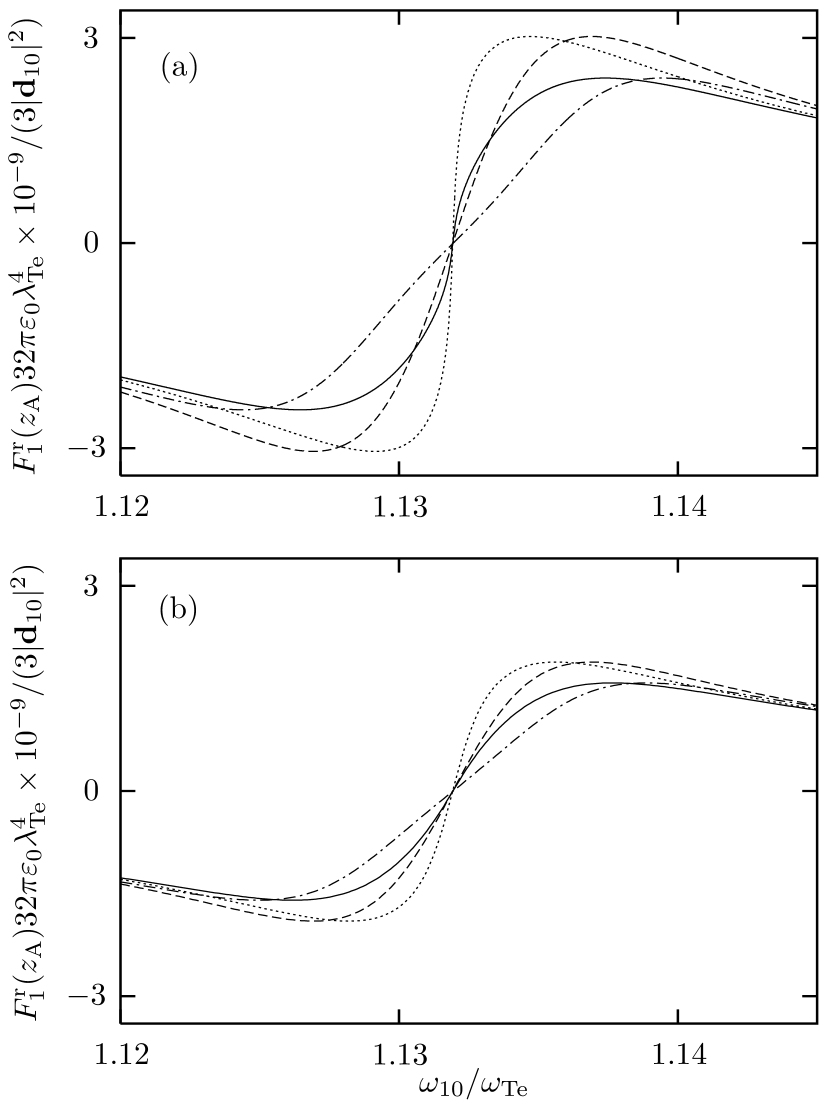
Figure 1: Resonant part of the CP force on an excited two-level atom that is situated at distance (a) $z_{\mathrm{A}}/\lambda_{\mathrm{Te}}$ $\!=$ $\!0.0075$ and (b) $z_{\mathrm{A}}/\lambda_{\mathrm{Te}}$ $\!=$ $\!0.009$ ($\lambda_{\mathrm{Te}}$ $\!=$ $\!2\pi c/\omega_{\mathrm{Te}}$) of a semi-infinite dielectric half space and whose transition dipole moment is perpendicular to the interface, as a function of the atomic transition frequency (solid lines), where $\omega_{\mathrm{Pe}}/\omega_{\mathrm{Te}}$ $\!=$ $\!0.75$, $\gamma_{\mathrm{e}}/\omega_{\mathrm{Te}}$ $\!=$ $\!0.01$, $\omega_{\mathrm{Te}}^{2}|\vec{d}_{10}|^{2}/(3\pi\hbar\varepsilon_{0}c^{3})$ $\!=$ $\!10^{-7}$. For comparison, both the perturbative result, i.e., $\delta\omega_{m}(z_{\mathrm{A}})$ $\!=$ $\!\Gamma_{m}(z_{\mathrm{A}})$ $\!=$ $\!0$ (dashed lines) and the results obtainable by only considering the effect of level shifting, i.e., $\Gamma_{m}(z_{\mathrm{A}})$ $\!=$ $\!0$ (dotted lines) or only considering the effect of level broadening, i.e., $\delta\omega_{m}(z_{\mathrm{A}})$ $\!=$ $\!0$ (dash-dotted lines) are shown.

It is worth noting that the additional position-dependence introduced via the frequency shifts and broadenings has the effect that even the ground-state force cannot be derived, in general, from a potential in the way prescribed by Eqs. (37) and (38) in Sec. 3.1. While the force as given by Eq. (55) can of course still be written as a (time-dependent) potential force provided that the force components as given by Eqs. (63)–(3.2) are irrotational vectors (which is indeed the case for, e.g., an atom in the presence of planarly, spherically or cylindrically multilayered media), there may be situations where this is not possible, implying that Eqs. (63)–(3.2) can not be derived from an energy expression in the way given by Eqs. (37) and (38) in principle.

Clearly, the above mentioned effects of level shifting and broadening can only become relevant when the atom is situated sufficiently close to a body surface. As already mentioned, when the frequency shifts and broadenings can be neglected, $\delta\omega_{m}(\vec{r}_{\mathrm{A}})$ $\!\to$ $\!0$, $\Gamma_{m}(\vec{r}_{\mathrm{A}})$ $\!\to$ $\!0$, then the dynamical result for the force components $\vec{F}_{m}(\vec{r}_{\mathrm{A}})$ calculated by using Eq. (63) together with Eqs. (3.2)–(3.2) simplifies to the perturbative one calculated from Eq. (38) together with Eqs. (42)–(45). If necessary, the level shifts could of course be easily introduced in the perturbative formulas by replacing the bare transition frequencies with the shifted ones [$\omega_{mn}$ $\!\mapsto$ $\!\tilde{\omega}_{mn}(\vec{r}_{\mathrm{A}})$]. On the contrary, introduction of the level broadening is not so straightforward. In particular, the results of the dynamical theory can not be reproduced from the perturbative results by making the replacement $\bm{\alpha}_{0}^{(0)}(\omega)$ $\!\mapsto$ $\!\bm{\alpha}_{0}(\vec{r}_{\mathrm{A}},\omega)$ in the off-resonant force components (as done, e.g., in Ref. Kryszewski92 ) and replacing the bare transition frequencies by complex ones according to $\omega_{mn}$ $\!\mapsto$ $\!\Omega_{mn}(\vec{r}_{A})$ in the resonant components. Hence, the perturbative results as given in Sec. 3.1 may be regarded as a reasonable approximation only for the ground-state CP force, which is solely determined by the off-resonant component $\vec{F}_{0}^{\mathrm{or}}(\mathbf{r}_{A})$ and thus effectively not influenced by level broadening.

4 Ground-state atom within magnetodielectric multilayer system

To study the competing effects of electric and magnetic properties of the bodies on the CP force, let us consider a ground-state atom placed within a magnetodielectric multilayer system. From the arguments given above, we base, for simplicity, the calculations on the perturbative analysis, calculating the ground-state vdW potential $U_{0}(\vec{r}_{A})$ $\!=$ $\!U_{0}^{\mathrm{or}}(\vec{r}_{A})$ according to Eq. (46) together with Eq. (48).

Figure 2: Sketch of the planar multilayer system.

The planar multilayer system can be characterized as a stack of $n$ $\!+$ $\!1$ layers labelled by $l$ ($l$ $\!=$ $0,\ldots,n$) of thicknesses $d_{l}$ with planar parallel boundary surfaces, where $\varepsilon(\vec{r},\omega)$ $\!=$ $\!\varepsilon_{l}(\omega)$ and $\mu(\vec{r},\omega)$ $\!=$ $\mu_{l}(\omega)$. The coordinate system is chosen such that the layers are perpendicular to the $z$ axis and extend from $z$ $\!=$ $\!0$ to $z$ $\!=$ $\!d_{l}$ for $l$ $\!\neq$ $\!0,n$ and from $z$ $\!=$ $\!0$ to $z$ $\!=$ $\!-\infty$ ($\infty$) for $l$ $\!=$ $\!0$ ($n$) (cf. Fig. 2, where the position $z$ $\!=$ $\!0$ refers to layer $j$). The scattering part of the Green tensor at imaginary frequencies for $\vec{r}$ and $\vec{r}^{\prime}$ in layer $j$ can be given by Chew95

$$\mathsf{G}^{(1)}(\vec{r},\vec{r}^{\prime},iu)=\int\mathrm{d}^{2}q\,e^{i\vec{q}\cdot(\vec{r}-\vec{r}^{\prime})}\mathsf{G}^{(1)}(\vec{q},z,z^{\prime},iu)$$ (74)

($\mathbf{q}\perp\mathbf{e}_{z}$). Here,

$$\mathsf{G}^{(1)}(\vec{q},z,z^{\prime},iu)=\frac{\mu_{j}(iu)}{8\pi^{2}b_{j}}\sum_{\sigma=s,p}\biggl{\{}\frac{r^{\sigma}_{j-}r^{\sigma}_{j+}e^{-2b_{j}d_{j}}}{D_{j}^{\sigma}}$$

$$\quad\times\,\Bigl{[}\vec{e}_{\sigma}^{+}\vec{e}_{\sigma}^{+}e^{-b_{j}(z-z^{\prime})}+\vec{e}_{\sigma}^{-}\vec{e}_{\sigma}^{-}e^{b_{j}(z-z^{\prime})}\Bigr{]}$$

$$\qquad+\frac{1}{D_{j}^{\sigma}}\Bigl{[}\vec{e}_{\sigma}^{+}\vec{e}_{\sigma}^{-}r^{\sigma}_{j-}e^{-b_{j}(z+z^{\prime})}$$

$$\qquad\qquad\quad+\vec{e}_{\sigma}^{-}\vec{e}_{\sigma}^{+}r^{\sigma}_{j+}e^{-2b_{j}d_{j}}e^{b_{j}(z+z^{\prime})}\Bigr{]}\biggr{\}}$$ (75)

for $j$ $\!>$ $\!0$, where

$$\vec{e}_{s}^{\pm}=\vec{e}_{q}\times\vec{e}_{z},\quad\vec{e}_{p}^{\pm}=-\frac{1}{k_{j}}(iq\vec{e}_{z}\pm b_{j}\vec{e}_{q})$$ (76)

($\vec{e}_{q}$ $\!=$ $\!\vec{q}/q$, $q$ $\!=$ $\!|\vec{q}|$) with

$$k_{j}=\frac{u}{c}\sqrt{\varepsilon_{j}(iu)\mu_{j}(iu)}$$ (77)

are the polarization vectors for $s$- and $p$-polarized waves propagating in the positive ($+$) and negative ($-$) $z$-directions, $r^{\sigma}_{j-}$ and $r^{\sigma}_{j+}$ are the generalized coefficients for reflection at the left/right boundary of layer $j$, which can be calculated with the aid of the recursive relations

$$r^{s}_{l\pm}=\frac{\left(\frac{\mu_{l\pm 1}}{b_{l\pm 1}}-\frac{\mu_{l}}{b_{l}}\right)+\left(\frac{\mu_{l\pm 1}}{b_{l\pm 1}}+\frac{\mu_{l}}{b_{l}}\right)e^{-2b_{l\pm 1}d_{l\pm 1}}r^{s}_{l\pm 1\pm}}{\left(\frac{\mu_{l\pm 1}}{b_{l\pm 1}}+\frac{\mu_{l}}{b_{l}}\right)+\left(\frac{\mu_{l\pm 1}}{b_{l\pm 1}}-\frac{\mu_{l}}{b_{l}}\right)e^{-2b_{l\pm 1}d_{l\pm 1}}r^{s}_{l\pm 1\pm}}\,,$$ (78)

$$r^{p}_{l\pm}=\frac{\left(\frac{\varepsilon_{l\pm 1}}{b_{l\pm 1}}-\frac{\varepsilon_{l}}{b_{l}}\right)+\left(\frac{\varepsilon_{l\pm 1}}{b_{l\pm 1}}+\frac{\varepsilon_{l}}{b_{l}}\right)e^{-2b_{l\pm 1}d_{l\pm 1}}r^{p}_{l\pm 1\pm}}{\left(\frac{\varepsilon_{l\pm 1}}{b_{l\pm 1}}+\frac{\varepsilon_{l}}{b_{l}}\right)+\left(\frac{\varepsilon_{l\pm 1}}{b_{l\pm 1}}-\frac{\varepsilon_{l}}{b_{l}}\right)e^{-2b_{l\pm 1}d_{l\pm 1}}r^{p}_{l\pm 1\pm}}$$ (79)

($l$ $\!=$ $\!1,\ldots,j$ for $r^{\sigma}_{l-}$, $l$ $\!=$ $\!j,\ldots,n$ $\!-$ $\!1$ for $r^{\sigma}_{l+}$, $r^{\sigma}_{0-}$ $\!=$ $\!r^{\sigma}_{n+}$ $\!=$ $\!0$),

$$b_{l}=\sqrt{\frac{u^{2}}{c^{2}}\ \varepsilon_{l}(iu)\mu_{l}(iu)+q^{2}}$$ (80)

is the imaginary part of the $z$-component of the wave vector in layer $l$, and

$$D_{j}^{\sigma}=1-r_{j-}^{\sigma}r_{j+}^{\sigma}e^{-2b_{j}d_{j}}.$$ (81)

Let the atom be situated in the otherwise empty layer $j$, i.e., $\varepsilon_{j}(iu)$ $\!=$ $\!\mu_{j}(iu)$ $\!\equiv$ $\!1$ and

$$b_{j}=\sqrt{\frac{u^{2}}{c^{2}}+q^{2}}\equiv b.$$ (82)

To calculate the vdW potential, we substitute Eq. (74) together with Eq. (4) into Eq. (46), thereby omitting irrelevant position-independent terms [recall that $U_{0}^{\mathrm{or}}(\vec{r}_{A})$ $\!=$ $\!U_{0}(\vec{r}_{A})$]. Evaluating the trace with the aid of the relations

$$\vec{e}_{s}^{\pm}\cdot\vec{e}_{s}^{\pm}=\vec{e}_{s}^{\pm}\cdot\vec{e}_{s}^{\mp}=1,$$ (83)

$$\vec{e}_{p}^{\pm}\cdot\vec{e}_{p}^{\pm}=1,\quad\vec{e}_{p}^{\pm}\cdot\vec{e}_{p}^{\mp}=-1-2\left(\frac{qc}{u}\right)^{2},$$ (84)

which directly follow from Eqs. (76), (77), and (82), we realize that the resulting integrand of the $\vec{q}$-integral only depends on $q$. Thus after introducing polar coordinates in the $q_{x}q_{y}$-plane, we can easily perform the angular integration, leading to

$$U_{0}(z_{\mathrm{A}})=\frac{\hbar\mu_{0}}{8\pi^{2}}\int_{0}^{\infty}\mathrm{d}u\,u^{2}\alpha_{0}^{(0)}(iu)\int_{0}^{\infty}\mathrm{d}q\,\frac{q}{b}$$

$$\quad\times\,\Biggl{\{}e^{-2bz_{\mathrm{A}}}\biggl{[}\frac{r_{j-}^{s}}{D_{j}^{s}}-\biggl{(}1+2\frac{q^{2}c^{2}}{u^{2}}\biggr{)}\frac{r_{j-}^{p}}{D_{j}^{p}}\biggr{]}$$

$$\qquad\quad+e^{-2b(d_{j}-z_{\mathrm{A}})}\biggl{[}\frac{r_{j+}^{s}}{D_{j}^{s}}-\biggl{(}1+2\frac{q^{2}c^{2}}{u^{2}}\biggr{)}\frac{r_{j+}^{p}}{D_{j}^{p}}\biggr{]}\Biggr{\}}.$$ (85)

Note that Eq. (4) and thus Eq. (4) also apply to the case $j$ $\!=$ $\!0$ if $d_{0}$ is formally set equal to zero ($d_{0}$ $\!\equiv$ $\!0$).

Equation (4) together with Eq. (48) and Eqs. (78)–(82) gives the vdW potential of a ground-state atom within a general planar magnetodielectric multilayer system in terms of the atomic polarizability and the generalized reflection coefficients. Note that instead of calculating these coefficients from the permittivities and permeabilities of the individual layers via Eqs. (78)–(80) (as we shall do in this paper), it is possible to determine them experimentally by appropriate reflectivity measurements (cf., e.g., Ref. Thakur04 ). The coefficients $D_{j}^{\sigma}$ [Eq. (83)] describe the effect of multiple reflections of radiation at the two boundaries of the vacuum layer $j$ the atom is placed in, as can be seen by expanding $D_{j}^{\sigma}$ according to

$$\frac{1}{D_{j}^{\sigma}}=\sum_{n=0}^{\infty}\big{(}r_{j-}^{\sigma}e^{-b_{j}d_{j}}r_{j+}^{\sigma}e^{-b_{j}d_{j}}\big{)}^{n}\,.$$ (86)

Multiple reflections within layer $j$ do obviously not occur if the atom is placed in one of the semi-infinite outer layers ($j$ $\!=$ $\!n$), so that Eq. (4) reduces to

$$U_{0}(z_{\mathrm{A}}) =\frac{\hbar\mu_{0}}{8\pi^{2}}\int_{0}^{\infty}\mathrm{d}u\,u^{2}\alpha_{0}^{(0)}(iu)\int_{0}^{\infty}\mathrm{d}q\,\frac{q}{b}e^{-2bz_{\mathrm{A}}}$$ (87)

$$\qquad\qquad\times\,\biggl{[}r_{n-}^{s}-\biggl{(}1+2\frac{q^{2}c^{2}}{u^{2}}\biggr{)}r_{n-}^{p}\biggr{]}.$$

4.1 Infinitely thick plate

Let us apply Eqs. (4) and (87) to some simple systems and begin with an atom in front of a sufficiently thick magnetodielectric plate which can be effectively regarded as a semi-infinite half space [$n$ $\!=$ $\!j$ $\!=$ $\!1$, $\varepsilon_{1}(\omega)$ $\!=$ $\!\mu_{1}(\omega)$ $\!\equiv$ $\!1$, $\varepsilon_{0}(\omega)$ $\!\equiv$ $\!\varepsilon(\omega)$, $\mu_{0}(\omega)$ $\!\equiv$ $\!\mu(\omega)$]. Using Eqs. (78) and (79) we find that the reflection coefficients in Eq. (87) read ($b_{0}$ $\!\equiv$ $\!b_{\mathrm{M}}$)

$$r_{n-}^{s} = \frac{\mu(iu)b-b_{\mathrm{M}}}{\mu(iu)b+b_{\mathrm{M}}}\,,$$ (88)

$$r_{n-}^{p} = \frac{\varepsilon(iu)b-b_{\mathrm{M}}}{\varepsilon(iu)b+b_{\mathrm{M}}}\,.$$ (89)

Note that Eq. (87) together with Eqs. (88) and (89) is equivalent to the result derived in Ref. Kryszewski92 semiclassically within the frame of linear response theory.

To further analyze Eqs. (87)–(89), let us model the permittivity by Eq. (73) and the permeability by

$$\mu(\omega)=1+\,\frac{\omega_{\mathrm{Pm}}^{2}}{\omega_{\mathrm{Tm}}^{2}-\omega^{2}-i\omega\gamma_{\mathrm{m}}}\,.$$ (90)

In the long-distance (retarded) limit, i.e., $z_{\mathrm{A}}$ $\!\gg\!$ $c/\omega_{\mathrm{A}}^{-}$, $z_{\mathrm{A}}$ $\!\gg$ $\!c/\omega_{\mathrm{M}}^{-}$ [$\omega_{\mathrm{A}}^{-}$ $\!=$ $\mathrm{min}(\{\omega_{k0}|k$ $\!=$ $\!1,2,\ldots\})$, $\omega_{\mathrm{M}}^{-}$ $\!=$ $\mathrm{min}(\omega_{\mathrm{Te}},$ $\!\omega_{\mathrm{Tm}})$], Eqs. (87)–(89) reduce to (see Appendix A)

$$U_{0}(z_{\mathrm{A}})=\frac{C_{4}}{z_{\mathrm{A}}^{4}}\,,$$ (91)

where

$$C_{4}= -\frac{3\hbar c\alpha_{0}^{(0)}(0)}{64\pi^{2}\varepsilon_{0}}\int_{1}^{\infty}\mathrm{d}v\,\left[\left(\frac{2}{v^{2}}-\frac{1}{v^{4}}\right)\right.$$

$$\quad\times\,\frac{\varepsilon(0)v-\sqrt{\varepsilon(0)\mu(0)-1+v^{2}}}{\varepsilon(0)v+\sqrt{\varepsilon(0)\mu(0)-1+v^{2}}}$$

$$\quad-\frac{1}{v^{4}}\,\left.\frac{\mu(0)v-\sqrt{\varepsilon(0)\mu(0)-1+v^{2}}}{\mu(0)v+\sqrt{\varepsilon(0)\mu(0)-1+v^{2}}}\right],$$ (92)

while in the short-distance (nonretarded) limit, i.e., $z_{\mathrm{A}}$ $\!\ll$ $\!c/\omega_{\mathrm{A}}^{+}$ and/or $z_{\mathrm{A}}$ $\!\ll$ $\!c/\omega_{\mathrm{M}}^{+}$ [$\omega_{\mathrm{A}}^{+}$ $\!=$ $\!\mathrm{max}(\{\omega_{k0}|k$ $\!=$ $\!1,2,\ldots\})$, $\omega_{\mathrm{M}}^{+}$ $\!=\!$ $\mathrm{max}(\omega_{\mathrm{Te}},$ $\!\omega_{\mathrm{Tm}})$], Eqs. (87)–(89) lead to (see Appendix A)

$$U_{0}(z_{\mathrm{A}})=-\ \frac{C_{3}}{z_{\mathrm{A}}^{3}}+\frac{C_{1}}{z_{\mathrm{A}}}\,,$$ (93)

where

$$C_{3}=\frac{\hbar}{16\pi^{2}\varepsilon_{0}}\int_{0}^{\infty}\mathrm{d}u\ \alpha_{0}^{(0)}(iu)\frac{\varepsilon(iu)-1}{\varepsilon(iu)+1}\geq 0$$ (94)

and

$$C_{1}=\ \frac{\mu_{0}\hbar}{16\pi^{2}}\int_{0}^{\infty}\mathrm{d}u\ u^{2}\alpha_{0}^{(0)}(iu)\biggl{\{}\frac{\varepsilon(iu)-1}{\varepsilon(iu)+1}$$

$$+\frac{\mu(iu)-1}{\mu(iu)+1}+\frac{2\varepsilon(iu)[\varepsilon(iu)\mu(iu)-1]}{[\varepsilon(iu)+1]^{2}}\biggr{\}}\geq 0.$$ (95)

It should be pointed out that this asymptotic behaviour also remains valid for multiresonance permittivities and permeabilities of Drude-Lorentz type. Clearly, in this case the minimum $\omega_{\mathrm{M}}^{-}$ and the maximum $\omega_{\mathrm{M}}^{+}$ are defined with respect to all matter resonances.

Inspection of Eq. (4.1) reveals that the coefficient $C_{4}$ in Eq. (91) for the long-distance behaviour of the vdW potential is negative (positive) for a purely electric (magnetic) plate, corresponding to an attractive (repulsive) force. For a genuinely magnetodielectric plate the situation is more complex. As the coefficient $C_{4}$ monotoneously decreases as a function of $\varepsilon(0)$ and monotoneously increases as a function of $\mu(0)$,

$$\frac{\partial C_{4}}{\partial\varepsilon(0)}<0,\quad\frac{\partial C_{4}}{\partial\mu(0)}>0,\quad$$ (96)

the border between the attractive and repulsive potential, i.e., $C_{4}$ $\!=$ $\!0$, can be marked by a unique curve in the $\varepsilon(0)\mu(0)$-plane, which is displayed in Fig. 3.

Figure 3: Border between attractive and repulsive long-distance vdW potentials of an atom in front of an infinitely thick magnetodielectric plate according to Eq. (4.1) ($C_{4}$ $\!=$ $\!0$). The broken curves show the asymptotic behaviour as given by Eqs. (99) (inset) and (4.1).

In the limits of weak and strong magnetodielectric properties the integral in Eq. (4.1) can be evaluated analytically. In the case of weak magnetodielectric properties, $\chi_{\mathrm{e}}(0)$ $\!\equiv$ $\!\varepsilon(0)$ $\!-1$ $\!\ll$ $\!1$ and $\chi_{\mathrm{m}}(0)$ $\!\equiv$ $\!\mu(0)$ $\!-$ $\!1$ $\!\ll$ $\!1$, the linear expansions

$$\frac{\varepsilon(0)v-\sqrt{\varepsilon(0)\mu(0)-1+v^{2}}}{\varepsilon(0)v+\sqrt{\varepsilon(0)\mu(0)-1+v^{2}}}$$

$$\qquad\simeq\left[\frac{1}{2}-\frac{1}{4v^{2}}\right]\chi_{\mathrm{e}}(0)-\frac{1}{4v^{2}}\chi_{\mathrm{m}}(0)$$ (97)

and

$$\frac{\mu(0)v-\sqrt{\varepsilon(0)\mu(0)-1+v^{2}}}{\mu(0)v+\sqrt{\varepsilon(0)\mu(0)-1+v^{2}}}$$

$$\qquad\simeq-\frac{1}{4v^{2}}\chi_{\mathrm{e}}(0)+\left[\frac{1}{2}-\frac{1}{4v^{2}}\right]\chi_{\mathrm{m}}(0)$$ (98)

lead to

$$C_{4}=-\frac{\hbar c\alpha_{0}^{(0)}(0)}{640\pi^{2}\varepsilon_{0}}\bigl{[}23\ \chi_{\mathrm{e}}(0)-7\chi_{\mathrm{m}}(0)\bigr{]}.$$ (99)

For strong magnetodielectric properties, i.e., $\varepsilon(0)$ $\!\gg$ $\!1$ and $\mu(0)$ $\!\gg$ $\!1$, we may approximately set, on noting that large values of $v$ are effectively suppressed in the integral in Eq. (4.1),

$$\sqrt{\varepsilon(0)\mu(0)-1+v^{2}}\simeq\sqrt{\varepsilon(0)\mu(0)}\,,$$ (100)

thus

$$C_{4}= -\frac{3\hbar c\alpha_{0}^{(0)}(0)}{64\pi^{2}\varepsilon_{0}}\biggl{[}-\,\frac{2}{Z^{3}}\mathrm{ln}(1\!+\!Z)+\frac{2}{Z^{2}}+\frac{4}{Z}\mathrm{ln}(1\!+\!Z)$$

$$-\frac{1}{Z}-\frac{4}{3}-Z+2Z^{2}-2Z^{3}\mathrm{ln}\biggl{(}1+\frac{1}{Z}\biggr{)}\biggr{]},$$ (101)

with $Z$ $\!\equiv$ $\!\sqrt{\mu(0)/\varepsilon(0)}$ denoting the static impedance of the material. Setting $C_{4}$ $\!=$ $\!0$ in Eqs. (99) and (4.1), we obtain the asymptotic behaviour of the border curve in the two limiting cases. The result shows that a repulsive vdW potential can be realized if $\chi_{\mathrm{m}}(0)/\chi_{\mathrm{e}}(0)$ $\!\geq$ $\!23/7$ $\!=$ $\!3.29$ in the case of weak magnetodielectric properties, and $\mu(0)/\varepsilon(0)$ $\!\geq$ $\!5.11$ ($Z$ $\!\geq$ $\!2.26$) in the case of strong magnetodielectric properties.

Apart from the different distance laws, the short-distance vdW potential, Eq. (93), differs from the long-distance potential, Eq. (91), in two respects. First, the relevant coefficients $C_{3}$ and $C_{1}$ are not only determined by the static values of the permittivity and the permeability, as is seen from Eqs. (94) and (4.1), and second, Eqs. (93)–(4.1) reveal that electric and magnetic properties give rise to potentials with different distance laws and signs [$C_{3}$ $\!>$ $\!0$ dominant (and $C_{1}$ $\!>$ $\!0$) if $\varepsilon$ $\!\neq$ $\!1$ and $\mu$ $\!=$ $\!1$, while $C_{3}$ $\!=$ $\!0$ and $C_{1}$ $\!>$ $\!0$ if $\varepsilon$ $\!=$ $\!1$ and $\mu$ $\!\neq$ $\!1$]. However, although for the case of a purely magnetic plate a repulsive vdW potential proportional to $1/z_{\mathrm{A}}$ is predicted, in practice the attractive $1/z_{\mathrm{A}}^{3}$ term will always dominate for sufficiently small values of $z_{\mathrm{A}}$, because of the always existing electric properties of the plate. Hence when in the long-distance limit the potential becomes repulsive due to sufficiently strong magnetic properties, then the formation of a potential wall at intermediate distances becomes possible. It is evident that with decreasing strength of the electric properties the maximum of the wall is shifted to smaller distances while increasing in height.

In the limiting case of weak electric properties, i.e., $\omega_{\mathrm{Pe}}/\omega_{\mathrm{Te}}$ $\!\ll$ $\!1$ and $\omega_{\mathrm{Pe}}/\omega_{\mathrm{Pm}}$ $\!\ll$ $\!1$ [recall Eqs. (73) and (90)] one can thus expect that the wall is situated within the short-distance range, so that Eqs. (93)–(4.1) can be used to determine both its position and height. From Eq. (93) we find that the wall maximum is at

$$z_{\mathrm{A}}^{\mathrm{max}}=\sqrt{\frac{3C_{3}}{C_{1}}}$$ (102)

and has a height of

$$U(z_{\mathrm{A}}^{\mathrm{max}})=\frac{2}{3}\sqrt{\frac{C_{1}^{3}}{3C_{3}}}\,.$$ (103)

In order to evaluate the integrals in Eqs. (94) and (4.1) for the coefficients $C_{3}$ and $C_{1}$, respectively, let us restrict our attention to the case of a two-level atom and disregard absorption ($\gamma_{\mathrm{e}}$ $\!\simeq$ $\!0$, $\!\gamma_{\mathrm{m}}$ $\!\simeq$ $\!0$). Straightforward calculation yields ($\omega_{\mathrm{Pe}}/\omega_{\mathrm{Te}}$ $\!\ll$ $\!1$, $\omega_{\mathrm{Pe}}/\omega_{\mathrm{Pm}}$ $\!\ll$ $\!1$)

$$C_{3}\simeq\frac{|\vec{d}_{01}|^{2}}{96\pi\varepsilon_{0}}\,\frac{\omega_{\mathrm{Pe}}^{2}}{\omega_{\mathrm{Te}}^{2}}\,\frac{\omega_{\mathrm{Te}}}{\omega_{10}\!+\!\omega_{\mathrm{Te}}}$$ (104)

and

$$C_{1}\simeq \,\frac{\mu_{0}\hbar}{16\pi^{2}}\int_{0}^{\infty}\mathrm{d}u\ u^{2}\alpha_{0}^{(0)}(iu)\left[\frac{\mu(iu)\!-\!1}{\mu(iu)\!+\!1}+\frac{\mu(iu)\!-\!1}{2}\right]$$

$$= \,\frac{\mu_{0}|\vec{d}_{01}|^{2}\omega_{\mathrm{Pm}}^{2}}{96\pi}\,\frac{\omega_{\mathrm{10}}(2\omega_{\mathrm{10}}+\omega_{\mathrm{Sm}}+\omega_{\mathrm{Tm}})}{(\omega_{\mathrm{10}}+\omega_{\mathrm{Sm}})(\omega_{\mathrm{10}}+\omega_{\mathrm{Tm}})}$$ (105)

[$\omega_{\mathrm{Sm}}$ $\!=\!$ $\!(\omega_{\mathrm{Tm}}^{2}$ $\!+$ $\!\frac{1}{2}\omega_{\mathrm{Pm}}^{2})^{1/2}$]. Substitution of Eqs. (104) and (4.1) into Eqs. (102) and (103), respectively, leads to

$$z_{\mathrm{A}}^{\mathrm{max}}= \,\frac{c}{\omega_{\mathrm{Pm}}}\frac{\omega_{\mathrm{Pe}}}{\omega_{\mathrm{Te}}}\sqrt{\frac{\omega_{\mathrm{Te}}(\omega_{10}+\omega_{\mathrm{Tm}})}{\omega_{10}(\omega_{10}+\omega_{\mathrm{Te}})}}$$

$$\quad\times\,\sqrt{\frac{3(\omega_{10}\!+\!\omega_{\mathrm{Sm}})}{(2\omega_{\mathrm{10}}+\omega_{\mathrm{Sm}}+\omega_{\mathrm{Tm}})}}$$ (106)

and

$$U(z_{\mathrm{A}}^{\mathrm{max}})= \,\frac{|\mathbf{d}_{01}|^{2}\omega_{\mathrm{Pm}}^{3}}{48\pi\varepsilon_{0}c^{3}}\,\frac{\omega_{\mathrm{Te}}}{\omega_{\mathrm{Pe}}}\sqrt{\frac{\omega_{10}+\omega_{\mathrm{Te}}}{\omega_{\mathrm{Te}}}}$$

$$\quad\times\,\left[\frac{\omega_{10}(2\omega_{10}\!+\!\omega_{\mathrm{Sm}}+\omega_{\mathrm{Tm}})}{3(\omega_{10}+\omega_{\mathrm{Sm}})(\omega_{10}+\omega_{\mathrm{Tm}})}\right]^{\frac{3}{2}}\,.$$ (107)

Note that consistency with the assumption of the wall occurring at short distances requires that $z_{\mathrm{A}}^{\mathrm{max}}$ $\!\ll$ $c/\omega_{\mathrm{M}}^{+}$—a condition which is easily fulfilled for sufficiently small values of $\omega_{\mathrm{Pe}}/\omega_{\mathrm{Pm}}$. Inspection of Eq. (4.1) shows that the height of the wall increases with $\omega_{\mathrm{Pm}}$, but decreases with increasing $\omega_{\mathrm{Tm}}$ or increasing $\omega_{\mathrm{Pe}}/\omega_{\mathrm{Te}}$ $\!=$ $\!\sqrt{\varepsilon(0)-1}$. Since the dependence of $U(z_{\mathrm{A}}^{\mathrm{max}})$ on $\omega_{\mathrm{Pm}}$ is seen to be much stronger than its dependence on $\omega_{\mathrm{Tm}}$, the wall height increases with $\omega_{\mathrm{Tm}}$ for given $\omega_{\mathrm{Pm}}/\omega_{\mathrm{Tm}}$ $\!=$ $\!\sqrt{\mu(0)-1}$.

Figure 4: The vdW potential of a ground-state two-level atom situated in front of an infinitely thick magnetodielectric plate is shown as a function of the distance between the atom and the plate for different values of $\omega_{\mathrm{Pm}}$ ($\omega_{\mathrm{Pe}}/\omega_{10}$ $\!=$ $\!0.75$, $\omega_{\mathrm{Te}}/\omega_{10}$ $\!=$ $\!1.03$, $\omega_{\mathrm{Tm}}/\omega_{10}$ $\!=$ $\!1$, $\gamma_{\mathrm{e}}/\omega_{10}$ $\!=$ $\!\gamma_{\mathrm{m}}/\omega_{10}$ $\!=$ $\!0.001$).

The distance-dependence of the vdW potential, as calculated from Eq. (87) together with Eqs. (88) and (89) for a two-level atom in front of a thick magnetodielectric plate whose permittivity and permeability are modelled by Eqs. (73) and (90), respectively, is illustrated in Fig. 4. The figure reveals that the results derived above for the case where the potential wall is observed in the short-distance range remain qualitatively valid also for larger distances. So it is seen that for sufficiently large values of $\omega_{\mathrm{Pm}}$ a potential wall begins to form and grows in height as $\omega_{\mathrm{Pm}}$ increases.

In view of left-handed materials (cf. Refs. Pendry99 ; Smith00 ; Veselago68 ), which simultaneously exhibit negative real parts of $\varepsilon(\omega)$ and $\mu(\omega)$ within some (real) frequency interval such that the real part of the refractive index becomes negative therein, the question may arise whether these materials would have an exceptional effect on the ground-state CP force. The answer is obviously no, because the ground-state vdW potential as given by Eq. (87) together with Eqs. (88) and (89) is expressed in terms of the always positive values of the permittivity and the permeability at imaginary frequencies. Clearly, the situation may change for an atom prepared in an excited state. In such a case, the vdW potential is essentially determined by the real part of the Green tensor [cf. Eqs. (3.2) and (67)]. When there are transition frequencies that lie in frequency intervals where the material behaves left-handed, then particularities may occur.

4.2 Plate of finite thickness

Let us now consider an atom in front of a magnetodielectric plate of finite thickness $d_{1}$ $\!\equiv\!$ $d$ [$n$ $\!=$ $\!j$ $\!=$ $\!2$, $\varepsilon_{1}(\omega)$ $\!\equiv$ $\!\varepsilon(\omega)$, $\mu_{1}(\omega)$ $\!\equiv$ $\!\mu(\omega)$, $\varepsilon_{0}(\omega)$ $\!=$ $\!\varepsilon_{2}(\omega)$ $\!\equiv$ $\!1$, $\mu_{0}(\omega)$ $\!=$ $\!\mu_{2}(\omega)$ $\!\equiv$ $\!1$]. Using Eqs. (78) and (79) we find that the reflection coefficients in Eq. (87) are now given by ($b_{1}$ $\!\equiv$ $\!b_{\mathrm{M}}$)

$$r_{n-}^{s} \!= \!\frac{[\mu^{2}(iu)b^{2}-b_{\mathrm{M}}^{2}]\tanh(b_{\mathrm{M}}d)}{2\mu(iu)bb_{\mathrm{M}}+[\mu^{2}(iu)b^{2}+b_{\mathrm{M}}^{2}]\tanh(b_{\mathrm{M}}d)}\,,\quad$$ (108)

$$r_{n-}^{p} \!= \!\frac{[\varepsilon^{2}(iu)b^{2}-b_{\mathrm{M}}^{2}]\tanh(b_{\mathrm{M}}d)}{2\varepsilon(iu)bb_{\mathrm{M}}+[\varepsilon^{2}(iu)b^{2}+b_{\mathrm{M}}^{2}]\tanh(b_{\mathrm{M}}d)}\,.$$ (109)

Typical examples of the vdW potential obtained by numerical evaluation of Eq. (87) [together with Eqs. (108) and (109)] for a two-level atom are shown in Fig. 5, revealing that for sufficiently strong magnetic properties the formation of a repulsive potential wall can also be observed for a magnetodielectric plate of finite thickness. In the figure, the medium parameters correspond to those which have already been found to support the formation of a repulsive potential wall in the case of an infinitely thick plate. We see that the qualitative behaviour of the vdW potential is independent of the layer thickness. In particular, all curves in Fig. 5 feature a repulsive long-range potential that leads to a potential wall of finite height, the potential becoming attractive at very short distances. However, the position and height of the wall are seen to vary with the thickness of the plate. While the position of the wall shifts only slightly as the plate thickness is changed from very small to very large values, the height of the wall reacts very sensitively as the plate thickness is varied. For small values of the thickness the potential height is very small, it increases towards a maximum, and then decreases asymptotically towards the value found for the infinitely thick plate as the thickness is increased further towards very large values. It is worth noting that there is an optimal plate thickness for creating a maximum potential wall. In this case the plate thickness is comparable to the position of the potential maximum—a case which is realized between the two extremes of infinitely thick and infinitely thin layer thickness.

Figure 5: The vdW potential of a ground-state two-level atom situated in front of a magnetodielectric plate is shown as a function of the distance between the body and the interface for different values of the plate thickness $d$ ($\omega_{\mathrm{Pe}}/\omega_{10}$ $\!=$ $\!0.75$, $\omega_{\mathrm{Te}}/\omega_{10}$ $\!=$ $\!1.03$, $\omega_{\mathrm{Pm}}/\omega_{10}$ $\!=$ $\!2$, $\omega_{\mathrm{Tm}}/\omega_{10}$ $\!=$ $\!1$, $\gamma_{\mathrm{e}}/\omega_{10}$ $\!=$ $\!\gamma_{\mathrm{m}}/\omega_{10}$ $\!=$ $\!0.001$).

Further insight can be gained by considering the two limiting cases of an infinitely thick and an asymptotically thin plate. It is obvious that the integration in Eq. (87) is effectively limited by the exponential factor $e^{-2bz_{\mathrm{A}}}$ to a circular region where $b$ $\!\lesssim$ $\!1/(2z_{\mathrm{A}})$. In particular, in the limit of a sufficiently thick plate, $d$ $\!\gg$ $\!z_{\mathrm{A}}$, the estimate

$$b_{\mathrm{M}}d\geq bd\sim\frac{d}{2z_{\mathrm{A}}}\gg 1$$ (110)

[recall Eqs. (80) and (82)] is valid within (the major part of) the effective region of integration, and one may hence make the approximation $\tanh(b_{\mathrm{M}}d)$ $\!\simeq$ $\!1$ in Eqs. (108) and (109), which then obviously reduce to Eqs. (88) and (89) valid for an infinitely thick plate. On the contrary, in the limit of an asymptotically thin plate, $\sqrt{\varepsilon(0)\mu(0)}d$ $\!\ll$ $\!z_{\mathrm{A}}$, we find that the inequalities

$$b_{\mathrm{M}}d \leq\sqrt{\varepsilon(iu)\mu(iu)}\,bd\leq\sqrt{\varepsilon(0)\mu(0)}\,bd$$

$$\leq\frac{\sqrt{\varepsilon(0)\mu(0)}d}{2z_{\mathrm{A}}}\ll 1$$ (111)

hold in the effective region of integration, and one may hence linearly expand the integrand in Eq. (87) in terms of $b_{\mathrm{M}}d$, which is equivalent to approximating the reflection coefficients (108) and (109) according to

$$r_{n-}^{s} \simeq \frac{\mu^{2}(iu)b^{2}-b_{\mathrm{M}}^{2}}{2\mu(iu)b}\,d\,,$$ (112)

$$r_{n-}^{p} \simeq \frac{\varepsilon^{2}(iu)b^{2}-b_{\mathrm{M}}^{2}}{2\varepsilon(iu)b}\,d\,.$$ (113)

As in the case of an infinitely thick plate, cf. Sec. 4.1, the dependence of the vdW potential on the atom-plate separation in the case of an asymptotically thin plate reduces to simple power laws in the long- and short-distance limits. In the long-distance limit, $z_{\mathrm{A}}$ $\!\gg$ $\!c/\omega_{\mathrm{A}}^{-}$, $z_{\mathrm{A}}$ $\!\gg$ $\!c/\omega_{\mathrm{M}}^{-}$, Eq. (87) together with Eqs. (112) and (113) reduces to (see Appendix A)

$$U(z_{\mathrm{A}})=\frac{D_{5}}{z_{\mathrm{A}}^{5}}\,,$$ (114)

where

$$D_{5}=-\frac{\hbar c\alpha_{0}^{(0)}(0)d}{160\pi^{2}\varepsilon_{0}}\,\biggl{[}\frac{14\varepsilon^{2}(0)-9}{\varepsilon(0)}-\frac{6\mu^{2}(0)-1}{\mu(0)}\biggr{]}\,,$$ (115)

while in the short-distance limit, $z_{\mathrm{A}}$ $\!\ll$ $\!c/\omega_{\mathrm{A}}^{+}$ and/or $z_{\mathrm{A}}$ $\!\ll$ $\!c/\omega_{\mathrm{M}}^{+}$, Eq. (87) together with Eqs. (112) and (113) can be approximated by (see Appendix A)

$$U(z_{\mathrm{A}})=-\frac{D_{4}}{z_{\mathrm{A}}^{4}}+\frac{D_{2}}{z_{\mathrm{A}}^{2}}\,,$$ (116)

where

$$D_{4}=\frac{3\hbar d}{64\pi^{2}\varepsilon_{0}}\int_{0}^{\infty}\mathrm{d}u\,\alpha_{0}^{(0)}(iu)\frac{\varepsilon^{2}(iu)-1}{\varepsilon(iu)}\geq 0$$ (117)

and

$$D_{2}=\frac{\mu_{0}\hbar d}{64\pi^{2}}\int_{0}^{\infty}\mathrm{d}u\,u^{2}\alpha_{0}^{(0)}(iu)\Biggl{\{}\frac{\varepsilon^{2}(iu)-1}{\varepsilon(iu)}$$

$$\hskip 25.83325pt+\frac{\mu^{2}(iu)-1}{\mu(iu)}+\frac{2[\varepsilon(iu)\mu(iu)-1]}{\varepsilon(iu)}\Biggr{\}}\geq 0\,.$$ (118)

Comparing the power laws (114) and (116) with those obtained for an infinitely thick plate, Eqs. (91) and (93), we see that the powers of $1/z_{\mathrm{A}}$ are universally increased by one. Again, we find that in the long-distance limit the vdW potential follows a power law that is independent of the material properties of the plate, the sign being determined by the relative strengths of the magnetic and electric properties (a purely electric plate creates an attractive vdW potential, while a purely magnetic plate gives rise to a repulsive one). And again the short-distance behaviours of the vdW potential for plates of different material properties (i.e., electric/magnetic) differ in both sign and leading power law (the repulsive potential in the case of a purely magnetic plate being weaker than the attractive potential in the case of a purely electric plate by two powers in the atom-plate separation). Interestingly, a similar behaviour, i.e., the same hierarchy of power laws and the same signs have been found for the vdW force between two atoms Sucher68 ; Boyer69 ; Farina02 and for the Casimir force between two semi-infinite half spaces Henkel04 . This is illustrated in Tab. 1, where the asymptotic power laws found for an atom interacting with an infinitely thick plate, Eqs. (91) and (4.1), and an asymptotically thin plate, Eqs. (114) and (4.2), are summarized and compared to those valid for the interactions between two atoms or two half spaces, respectively.

distance	short		long
polarizability	$\mathrm{e}\leftrightarrow\mathrm{e}$	$\mathrm{e}\leftrightarrow\mathrm{m}$	$\mathrm{e}\leftrightarrow\mathrm{e}$	$\mathrm{e}\leftrightarrow\mathrm{m}$
atom $\leftrightarrow$ h.s.	$$-\frac{1}{z^{4}}$$	$$+\frac{1}{z^{2}}$$	$$-\frac{1}{z^{5}}$$	$$+\frac{1}{z^{5}}$$
atom $\leftrightarrow$ thin plate	$$-\frac{1}{z^{5}}$$	$$+\frac{1}{z^{3}}$$	$$-\frac{1}{z^{6}}$$	$$+\frac{1}{z^{6}}$$
atom $\leftrightarrow$ atom	$$-\frac{1}{z^{7}}$$	$$+\frac{1}{z^{5}}$$	$$-\frac{1}{z^{8}}$$	$$+\frac{1}{z^{8}}$$
h.s. $\leftrightarrow$ h.s.	$$-\frac{1}{z^{3}}$$	$$+\frac{1}{z}$$	$$-\frac{1}{z^{4}}$$	$$+\frac{1}{z^{4}}$$

Table 1: Signs and asymptotic power laws of the forces between various polarizable objects. In the table heading, $\mathrm{e}$ stands for a purely electric object and $\mathrm{m}$ for a purely magnetic one. The signs $+$ and $-$ denote repulsive and attractive forces, respectively. Half space is abbreviated by h.s..

For weak magnetodielectric properties, the similarity of the results displayed in Tab. 1 can be regarded as being a consequence of the additivity of vdW-type interactions. In fact, in this case (which for a gaseous medium of given atomic species corresponds to a sufficiently dilute gas) all results of the table can be derived from the vdW interaction of two single atoms via pairwise summation. The additivity can explicitly be seen when comparing the result found for an asymptotically thin plate with that of an infinitely thick plate in the case of weak magnetodielectric properties [$\chi_{\mathrm{e}}(iu)$ $\!\equiv$ $\!\varepsilon(iu)$ $\!-1$ $\!\ll$ $\!1$, $\chi_{\mathrm{m}}(iu)$ $\!\equiv$ $\!\mu(iu)$ $\!-$ $\!1$ $\!\ll$ $\!1$]. Making a linear expansion in $\chi_{\mathrm{e}}(iu)$ and $\chi_{\mathrm{m}}(iu)$, we find that the vdW potential of an infinitely thick plate, Eq. (87) together with Eqs. (88) and (89), reduces to

$$\Delta_{1}U(z_{\mathrm{A}}) =-\frac{\hbar\mu_{0}}{8\pi^{2}}\int_{0}^{\infty}\!\!\mathrm{d}u\,u^{2}\alpha^{(0)}(iu)\int_{0}^{\infty}\!\!\mathrm{d}q\,\frac{q}{b}e^{-2bz_{\mathrm{A}}}$$

$$\hskip 51.6665pt\times\,\Biggl{\{}\Biggl{[}\biggl{(}\frac{bc}{u}\biggr{)}^{2}-1+\frac{1}{2}\biggl{(}\frac{u}{bc}\biggr{)}^{2}\Biggr{]}\chi_{\mathrm{e}}(iu)$$

$$\hskip 77.49976pt-\Biggl{[}1-\frac{1}{2}\biggl{(}\frac{u}{bc}\biggr{)}^{2}\Biggr{]}\chi_{\mathrm{m}}(iu)\Biggr{\}}\,,$$ (119)

while the vdW potential of an asymptotically thin plate, Eq. (87) together with Eqs. (112) and (113), can be approximated by

$$\Delta_{1}U^{d}(z_{\mathrm{A}}) =-\frac{\hbar\mu_{0}d}{4\pi^{2}}\int_{0}^{\infty}\!\!\mathrm{d}u\,u^{2}\alpha^{(0)}(iu)\int_{0}^{\infty}\!\!\mathrm{d}q\,qe^{-2bz_{\mathrm{A}}}$$

$$\hskip 8.61108pt\times\,\Biggl{\{}\Biggl{[}\biggl{(}\frac{bc}{u}\biggr{)}^{2}-1+\frac{1}{2}\biggl{(}\frac{u}{bc}\biggr{)}^{2}\Biggr{]}\chi_{\mathrm{e}}(iu)$$

$$\hskip 34.44434pt-\Biggl{[}1-\frac{1}{2}\biggl{(}\frac{u}{bc}\biggr{)}^{2}\Biggr{]}\chi_{\mathrm{m}}(iu)\Biggr{\}}\,.$$ (120)

Comparison of Eqs. (4.2) and (4.2) shows that for weakly magnetodielectric media the vdW potential of an infinitely thick plate is simply the integral over an infinite number of thin-plate vdW potentials,

$$U_{0}(z_{\mathrm{A}})=\int_{z_{\mathrm{A}}}^{\infty}\frac{\mathrm{d}z}{d}\,U^{d}_{0}(z).$$ (121)

In the case of media with stronger magnetodielectric properties many-body interactions may be thought of as preventing the vdW potential from being additive so that a relation of the type of Eq. (121) is not true in general. As a consequence, the coefficients of the asymptotic power laws in Tab. 1 can not be related to each other via simple additivity arguments in general. However, we note from Tab. 1 that the consideration of many-body corrections only changes the coefficients of the asymptotic power laws, not the power laws themselves.

4.3 Planar cavity

Finally, let us consider an atom placed within the simplest type of planar cavity, i.e., between two identical infinitely thick magnetodielectric plates which are separated by a distance $d_{1}$ $\!\equiv$ $\!s$ [$n$ $\!=$ $\!2$, $j$ $\!=$ $\!1$, $\varepsilon_{1}(\omega)$ $\!=$ $\!\mu_{1}(\omega)$ $\!\equiv$ $\!1$, $\varepsilon_{0}(\omega)$ $\!=$ $\!\varepsilon_{2}(\omega)$ $\!\equiv$ $\varepsilon(\omega)$, $\mu_{0}(\omega)$ $\!=$ $\!\mu_{2}(\omega)$ $\!\equiv$ $\!\mu(\omega)$]. From Eqs. (78) and (79) it then follows that the reflection coefficients in Eq. (4) are given by ($b_{0}$ $\!=$ $\!b_{2}$ $\!\equiv$ $b_{\mathrm{M}}$)

$$r_{j-}^{s}=r_{j+}^{s}=\frac{\mu(iu)b-b_{\mathrm{M}}}{\mu(iu)b+b_{\mathrm{M}}}\,,$$ (122)

$$r_{j-}^{p}=r_{j+}^{p}=\frac{\varepsilon(iu)b-b_{\mathrm{M}}}{\varepsilon(iu)b+b_{\mathrm{M}}}\,.$$ (123)

Figure 6: The vdW potential of a ground-state two-level atom situated between two infinitely thick (a) magnetodielectric plates ($\omega_{\mathrm{Pe}}/\omega_{10}$ $\!=$ $\!0.75$, $\omega_{\mathrm{Te}}/\omega_{10}$ $\!=$ $\!1.03$, $\omega_{\mathrm{Pm}}/\omega_{10}$ $\!=$ $\!2$, $\omega_{\mathrm{Tm}}/\omega_{10}$ $\!=$ $\!1$, $\gamma_{\mathrm{e}}/\omega_{10}$ $\!=$ $\!\gamma_{\mathrm{m}}/\omega_{10}$ $\!=$ $\!0.001$) (b) dielectric plates [$\mu(\omega)$ $\!\equiv$ $\!1$, other parameters as in (a)], (c) magnetic plates [$\varepsilon(\omega)$ $\!\equiv$ $\!1$, other parameters as in (a)], which are separated by a distance $s$ $\!=$ $\!15c/\omega_{10}$, is shown as a function of the position of the atom.

Examples of the vdW potential of a two-level atom between two identical infinitely thick magnetodieletric plates as calculated from Eq. (4) together with Eqs. (122) and (123) are plotted in Fig. 6. It is seen that the attractive (repulsive) potentials associated with each of two purely electric (magnetic) plates combine to an infinite potential wall (well) at the center of the cavity. Hence, a potential well of finite depth at the center of the cavity can be realized in the case of two genuinely magnetodielectric plates of sufficiently strong magnetic properties as shown in the figure. Provided that appropriate materials would be available, this feature could in principle be used for the trapping and guiding of atoms.

5 Summary and Conclusions

Within the framework of exact macroscopic QED in linear, causal media, we have given a unified theory of the CP force acting on an atom when placed near an arbitrary arrangement of dispersing and absorbing magnetodielectric bodies. We have considered both the familiar perturbative approach to the problem, where the atom-field coupling energy calculated in lowest-order perturbation theory is regarded as the potential associated with the CP force acting on the atom prepared in an energy eigenstate, and a dynamical approach based on the Lorentz force averaged with respect to the body-assisted electromagnetic vacuum and the internal motion of the atom. In particular, the theory allows to extend the quantum mechanical calculation of the interaction energy to the realistic case of material dispersion and absorption—a case for which standard mode expansion of the electromagnetic field runs into difficulties. So, the theory yields the vdW potential in terms of the electromagnetic-field scattering Green tensor and the lowest-order atomic polarizability in a natural manner, without borrowing arguments from other theories such as the widely used linear response theory.

In contrast to the perturbative treatment of the CP force, the dynamical treatment allows for including arbitrary excited atomic states, their temporal evolution and thus transient components of the force, and the influence of the body-induced shifting and broadening of the atomic transitions on the force. Whereas level shifting can, at least for very small atom-body distances, noticeably modify both the resonant and the off-resonant force components, level broadening effectively affects only the resonant components. Thus the perturbative treatment may be justified for the purely off-resonant ground-state force, while being inadequate for the excited-state force containing resonant components (leaving aside its obvious inablity to describe the transient nature of excited-state components).

Finally, we have applied the theory to analyze the competing effects of the electric and magnetic properties on the CP force acting on a ground-state atom placed within a magnetodielectric multilayer system, studying the corresponding vdW potential for the cases of thick and thin plates as well as a planar cavity. In close analogy to the vdW interaction between two atoms or the Casimir force between two plates, the electric and magnetic properties compete in creating attractive and repulsive force components, respectively. In particular, if the atom interacts with a magnetodielectric plate of sufficiently strong magnetic properties, a potential wall can be formed. We have given conditions for the creation of such a wall and shown that there is an optimal plate thickness for maximizing the height of the wall. Placing the atom between two magnetodielectric plates each of which giving rise to a potential wall, one can combine the two potentials to a potential well. Needless to say that the thorough understanding of the interplay of electric and magnetic material properties can serve as a roadmap showing desirable directions of research in material design when aiming at shaping vdW potentials in a controlled way.

Appendix A Long- and short-distance limits

The long-distance (short-distance) limit corresponds to separation distances $z_{\mathrm{A}}$ between the atom and the multilayer system which are much greater (smaller) than the wavelenghts corresponding to typical frequencies of the atom and the multilayer system. To obtain approximate results for the two limiting cases, let us analyze the $u$-integral in Eq. (87) in a little more detail and begin with the long-distance limit, i.e.,

$$z_{\mathrm{A}}\gg\frac{c}{\omega_{\mathrm{A}}^{-}}\,,\quad z_{\mathrm{A}}\gg\frac{c}{\omega_{\mathrm{M}}^{-}}\,,$$ (124)

where $\omega_{\mathrm{A}}^{-}$ $\!=$ $\!\mathrm{min}(\{\omega_{k0}|k$ $\!=$ $\!1,2\ldots\})$ is the lowest atomic transition frequency, and $\omega_{\mathrm{M}}^{-}$ $\!=$ $\!\mathrm{min}(\omega_{\mathrm{Te}},\omega_{\mathrm{Tm}})$ is the lowest medium resonance frequency. For convenience, we introduce the new integration variable

$$v=\frac{cb}{u}$$ (125)

and transform the integral according to

$$\int_{0}^{\infty}\mathrm{d}u \int_{0}^{\infty}\mathrm{d}q\,\frac{q}{b}\,e^{-2bz_{\mathrm{A}}}\ldots$$

$$\mapsto\int_{1}^{\infty}\mathrm{d}v\int_{0}^{\infty}\mathrm{d}u\,\frac{u}{c}\,e^{-2z_{\mathrm{A}}vu/c}\ldots\ ,$$ (126)

where $b_{\mathrm{M}}$ has to be replaced according to

$$b_{\mathrm{M}}\mapsto\frac{u}{c}\,\sqrt{\varepsilon(iu)\mu(iu)-1+v^{2}}.$$ (127)

Inspection of Eqs. (87) together with Eqs. (88) and (89), or Eqs. (112) and (113), respectively, as well as Eq. (A) reveals that the frequency interval giving the main contribution to the respective $u$-integral is determined by a set of effective cutoff functions, namely

$$f(u)=e^{-2z_{\mathrm{A}}u/c},$$ (128)

$$g_{k}(u)=\frac{1}{1+(u/\omega_{k0})^{2}}\,,$$ (129)

which enter via the atomic polarizability, cf. Eq. (48), and

$$h_{\mathrm{e}}(u)=\frac{1}{1+(u/\omega_{\mathrm{Te}})^{2}}\,,$$ (130)

$$h_{\mathrm{m}}(u)=\frac{1}{1+(u/\omega_{\mathrm{Tm}})^{2}}\,,$$ (131)

which enter the reflection coefficients as given by Eqs. (88) and (89), or Eqs. (112) and (113), respectively, via $\varepsilon(iu)$ and $\mu(iu)$, cf. Eqs. (73) and (90). The cutoff functions obviously give their main contributions in regions, where

$$\hskip 43.05542ptu\lesssim\frac{c}{2z_{\mathrm{A}}} \mathrm{for} \quad f(u),\hskip 43.05542pt$$ (132)

$$\hskip 43.05542ptu\lesssim\omega_{k0} \mathrm{for} \quad g_{k}(u),\hskip 43.05542pt$$ (133)

$$\hskip 43.05542ptu\lesssim\omega_{\mathrm{Te}} \mathrm{for} \quad h_{\mathrm{e}}(u),\hskip 43.05542pt$$ (134)

$$\hskip 43.05542ptu\lesssim\omega_{\mathrm{Tm}} \mathrm{for} \quad h_{\mathrm{m}}(u).\hskip 43.05542pt$$ (135)

Combining Eqs. (132)–(135) with Eq. (124), we find that the function $f(u)$ effectively limits the $u$-integration to a region where

$$\frac{u}{\omega_{k0}}\leq\frac{u}{\omega_{\mathrm{A}}^{-}}\lesssim\frac{c}{2z_{\mathrm{A}}\omega_{\mathrm{A}}^{-}}\ll 1,$$ (136)

$$\frac{u}{\omega_{\mathrm{Te}}}\leq\frac{u}{\omega_{\mathrm{M}}^{-}}\lesssim\frac{c}{2z_{\mathrm{A}}\omega_{\mathrm{M}}^{-}}\ll 1,$$ (137)

$$\frac{u}{\omega_{\mathrm{Tm}}}\leq\frac{u}{\omega_{\mathrm{M}}^{-}}\lesssim\frac{c}{2z_{\mathrm{A}}\omega_{\mathrm{M}}^{-}}\ll 1.$$ (138)

Performing a leading-order expansion of the integrand in Eq. (87) in terms of the small quantities $u/\omega_{k0}$, $u/\omega_{\mathrm{Te}}$, and $u/\omega_{\mathrm{Tm}}$, we may set

$$\alpha_{0}^{(0)}(iu)\simeq\alpha_{0}^{(0)}(0),\ \varepsilon(iu)\simeq\varepsilon(0),\ \mu(iu)\simeq\mu(0).$$ (139)

Combining Eqs. (125)–(127) and Eq. (139) with Eq. (87) together with Eqs. (88) and (89), or Eqs. (112) and (113), respectively, and evaluating the remaining $u$-integrals we arrive at Eq. (91) [together with Eq. (4.1)] and Eq. (114) [together with Eq. (115)].

The short-distance limit, on the contrary, is defined by

$$z_{\mathrm{A}}\ll\frac{c}{\omega_{\mathrm{A}}^{+}}\quad\mathrm{and/or}\quad z_{\mathrm{A}}\ll\frac{c}{\omega_{\mathrm{M}}^{+}}\,,$$ (140)

where $\omega_{\mathrm{A}}^{+}$ $\!=$ $\!\mathrm{max}(\{\omega_{k0}|k$ $\!=$ $\!1,2,\ldots\})$ is the highest inneratomic transition frequency and $\omega_{\mathrm{M}}^{+}$ $\!=\!$ $\mathrm{max}(\omega_{\mathrm{Te}},\omega_{\mathrm{Tm}})$ is the highest medium resonance frequency. Again, it is convenient to change the integration variables in Eq. (87), but now we transform according to

$$\int_{0}^{\infty}\mathrm{d}u \int_{0}^{\infty}\mathrm{d}q\,\frac{q}{b}\,e^{-2bz_{\mathrm{A}}}\ldots$$

$$\mapsto\int_{0}^{\infty}\mathrm{d}u\,\int_{u/c}^{\infty}\mathrm{d}b\,e^{-2bz_{\mathrm{A}}}\ldots\ ,$$ (141)

where $b_{\mathrm{M}}$ has to be replaced according to

$$b_{\mathrm{M}}\mapsto\sqrt{\frac{u^{2}}{c^{2}}\big{[}\varepsilon(iu)\mu(iu)-1\big{]}+b^{2}}\ .$$ (142)

Combining Eqs. (132)–(135) with Eq. (140) reveals that the functions $g_{k}(u)$, $h_{\mathrm{e}}(u)$, and $h_{\mathrm{m}}(u)$ limit the $u$-integration to a region where

$$\frac{z_{\mathrm{A}}u}{c}\lesssim\frac{z_{\mathrm{A}}\omega_{\mathrm{A}}^{+}}{c}\ll 1$$ (143)

and/or

$$\frac{z_{\mathrm{A}}u}{c}\lesssim\frac{z_{\mathrm{A}}\omega_{\mathrm{M}}^{+}}{c}\ll 1.$$ (144)

A valid approximation to the $u$-integral in Eq. (87) can hence be obtained by performing a Taylor exansion in $z_{\mathrm{A}}u/c$. To that end, we apply the transformation (A) to Eq. (87) together with Eqs. (88) and (89), or Eqs. (112) and (113), respectively, retain only the leading-order terms in $u/(cb)$ (corresponding to the leading-order terms in $z_{\mathrm{A}}u/c$ in the $u$-integral) and carry out the $b$-integral. After again discarding higher-order terms in $z_{\mathrm{A}}u/c$, we arrive at Eq. (93) [together with Eqs. (94) and (4.1)] and Eq. (116) [together with Eqs. (117) and (4.2)], respectively.

References

• (1) D. Raskin, P. Kusch, Phys. Rev. 179, 3, 179 (1969); A. Shih, D. Raskin, P. Kusch, Phys. Rev. A 9, 2, 652 (1974); A. Shih, ibid. 9, 4, 1507 (1974); A. Shih, V. A. Parsegian, idid. 12, 3, 835 (1975).
• (2) C. I. Sukenik, M. G. Boshier, D. Cho, V. Sandoghdar, and E. A. Hinds, Phys. Rev. Lett. 70, 5, 560 (1993); A. Anderson, S. Haroche, E. A . Hinds, W. Jhe, and D. Meschede, Phys. Rev. A 37, 9, 3594 (1988).
• (3) F. Shimizu, Phys. Rev. Lett. 86, 6, 987 (2001); V. Druzhinina and M. DeKieviet, Phys. Rev. Lett. 91, 193202 (2003).
• (4) V. Sandoghdar, C. I. Sukenik, E. A. Hinds, and S. Haroche, Phys. Rev. Lett. 68, 23, 3432 (1992); M. Marrocco, M. Weidinger, R. T. Sang, and H. Walther, Phys. Rev. Lett. 81, 26, 5784 (1998); M. A. Wilson, P. Bushev, J. Eschner, F. Schmidt-Kaler, C. Becher, R. Blatt, and U. Dorner, Phys. Rev. Lett. 91, 21, 213602 (2003); P. Bushev, A. Wilson, J. Eschner, C. Raab, F. Schmidt-Kaler, C. Becher, and R. Blatt, ibid. 92, 22, 223602 (2004).
• (5) M. Oria, M. Chevrollier, D. Bloch, M. Fichet, and M. Ducloy, Europhy. Lett. 14, 6, 527 (1991); M. Chevrollier, D. Bloch, G. Rahmat, and M. Ducloy, Opt. Lett. 16, 23, 1879 (1991); M. Chevrollier, M. Fichet, M. Oria, G. Rahmat, D. Bloch, and M. Ducloy, J. Phys. II France 2, 631 (1992); M. Gorris-Neveux, P. Monnot, M. Fichet, M. Ducloy, and R. Barbé, J. C. Keller, Opt. Commun. 134, 85 (1997); H. Failache, S. Saltiel, M. Fichet, D. Bloch, and M. Ducloy, Phys. Rev. Lett. 83, 26, 5467 (1999); M. Boustimi, B. Viaris de Lesegno, J. Baudon, J. Robert, and M. Ducloy, Phys. Rev. Lett. 86, 13, 2766 (2001); H. Failache, S. Saltiel, M. Fichet, D. Bloch, and M. Ducloy, Eur. Phys. J. D 23, 237 (2003).
• (6) L. W. Bruch, Surf. Sc. 125, 194 (1983).
• (7) K. Autumn, M. Sitti, Y. A. Liang, A. M. Peattie, W. R. Hansen, S. Sponberg, T. W. Kelly, R. Fearing, J. N. Israelachvili, R. J. Full, PNAS 99, 19, 12252 (2002).
• (8) A. B. Kesel, A. Martin, T. Seidl, Smart Mater. Struct. 13, 512 (2004).
• (9) G. Binnig, C. Gerber, C. F. Quate, Phys. Rev. Lett. 56, 9, 930 (1986); for a review see F. J. Giessibl, Rev. Mod. Phys. 75, 949 (2003).
• (10) C. S. Adams, M. Sigel, J. Mlynek, Phys. Rep. 240, 143 (1994).
• (11) F. Shimizu, J.-i. Fujita, Phys. Rev. Lett. 88, 12, 123201 (2002).
• (12) V. I. Balykin, V. S. Letokhov, Y. B. Ovchinnikov, A. I. Sidorov, Phys. Rev. Lett. 60, 21, 2137 (1988).
• (13) H. B. G. Casimir and D. Polder, Phys. Rev. 73, 360 (1948).
• (14) G. Barton, J. Phys. B, 7, 16, 2134 (1974); D. Meschede, W. Jhe, and E. A. Hinds, Phys. Rev. A 41, 3, 1587 (1990).
• (15) T. Nakajima, P. Lambropoulos, and H. Walther, Phys. Rev. A 56, 6, 5100 (1997).
• (16) Y. Tikochinsky and L. Spruch, Phys. Rev. A 48, 6, 4223 (1993).
• (17) I.V. Bondarev and P. Lambin, Solid State Commun. 132, 3-4, 203 (2004).
• (18) F. Zhou and L. Spruch, Phys. Rev. A 52, 297 (1995).
• (19) S. Y. Buhmann, Ho Trung Dung, and D.-G. Welsch, J. Opt. B: Quantum Semicl. Opt. 6, 127 (2004).
• (20) S. Y. Buhmann, L. Knöll, D.-G. Welsch, and Ho Trung Dung, Phys. Rev. A 70, 052117 (2004).
• (21) A. D. McLachlan, Proc. R. Soc. London Ser. A 271, 387 (1963).
• (22) A. D. McLachlan, Mol. Phys. 7, 381 (1963); G. S. Argawal, Phys. Rev. A 11, 1, 243 (1975).
• (23) J. M. Wylie and J. E. Sipe, Phys. Rev. A 30, 1185 (1984).
• (24) J. M. Wylie and J. E. Sipe, Phys. Rev. A 32, 2030 (1985).
• (25) C. Henkel, V. Sandoghdar, Opt. Commun. 158, 250 (1998).
• (26) A. D. McLachlan, Proc. R. Soc. London Ser. A 274, 80 (1963).
• (27) C. Henkel, K. Joulain, J.-P. Mulet, J. J. Greffet, J. Opt. A: Pure Appl. Opt. 4, 109 (2002).
• (28) M.-P. Gorza, S. Saltiel, H. Failache, M. Ducloy, Eur. Phys. J. D 15, 113 (2001).
• (29) S. Kryszewski, Mol. Phys. 78, 5, 1225 (1993).
• (30) G. Feinberg and J. Sucher, Phys. Rev. A 2, 6, 2395 (1970); for an extension see E. Lubkin, Phys. Rev. A 4, 1, 416 (1971).
• (31) G. Feinberg and J. Sucher, J. Chem. Phys. 48, 7, 3333 (1968).
• (32) T. H. Boyer, Phys. Rev. 180, 1, 19 (1969).
• (33) C. Farina, F. C. Santos, and A. C. Tort, J. Phys. A 35, 2477 (2002); Am. J. Phys. 70, 4, 421 (2002).
• (34) C. Henkel and K. Joulain, e-print quant-ph/0407153; cf. also M. S. Tomǎs, e-print quant-ph/0410057.
• (35) O. Kenneth, I. Klich, A. Mann, and M. Revzen, Phys. Rev. Lett. 89, 3, 033001 (2002); D. Iannuzzi and F. Capasso, Phys. Rev. Lett. 91, 2, 029101 (2003); for a reply see O. Kenneth, I. Klich, A. Mann, and M. Revzen, Phys. Rev. Lett. 91, 2, 029102 (2003).
• (36) Y.-y. Lin, I. Teper, C. Chin, and V. Vuletić, Phys. Rev. Lett. 92, 5, 050404 (2004).
• (37) J. B. Pendry, A. J. Holden, D. J. Robbins, and W. J. Stewart, IEEE Trans. Microwave Theory Tech. 47, 11, 2075 (1999).
• (38) D. R. Smith, W. J. Padilla, D. C. Vier, S. C. Nemat-Nasser, and S. Schultz, Phys. Rev. Lett. 84, 18, 4184 (2000).
• (39) Ho Trung Dung, S. Y. Buhmann, L. Knöll, D.-G. Welsch, S. Scheel, and J. Kästel, Phys. Rev. A 68, 043816 (2003).
• (40) D. P. Craig and T. Thirunamachandran Molecular Quantum Electrodynamics (Academic Press, New York, 1984).
• (41) H. Friedrich, G. Jacobi, C. G. Meister, Phys. Rev. A 65, 032902 (2002).
• (42) V. G. Veselago, Sov. Phys. Usp. 10, 509 (1968).
• (43) W. C. Chew, Waves and Fields in Inhomogeneous Media (IEEE Press, New York, 1995), Secs. 2.1.3, 2.1.4, and 7.4.2.
• (44) K. P. Thakur and W. S. Holmes, IEEE Trans. Microwave Theory Tech. 52, 1, 76 (2004).
• (45) W. Vogel, D.-G. Welsch, and S. Wallentowitz, Quantum Optics, An Introduction (Wiley-VCH, Berlin, 2001).