A model of deterministic detector with dynamical decoherence

Abstract

We discuss a deterministic model of detector coupled to a two-level system (a qubit). The detector is a quasi-classical object whose dynamics is described by the kicked rotator Hamiltonian. We show that in the regime of quantum chaos the detector acts as a chaotic bath and induces decoherence of the qubit. We discuss the dephasing and relaxation rates and demonstrate that several features of Ohmic baths can be reproduced by our fully deterministic model. Moreover, we show that, for strong enough qubit-detector coupling, the dephasing rate is given by the rate of exponential instability of the detector’s dynamics, that is, by the Lyapunov exponent of classical motion. Finally, we discuss the measurement in the regimes of strong and weak qubit-detector coupling. For the case of strong coupling the detector performs a measurement of the up/down state of the qubit. In the case of weak coupling, due to chaos, the dynamical evolution of the detector is strongly sensitive to the state of the qubit. However, in this case it is unclear how to extract a signal from any measurement with a coarse-graining in the phase space on a size much larger than the Planck cell.

I Introduction

The long-standing problem of quantum measurement braginsky ; giulini ; pascazio has recently gained a renewed interest due to its relevance for quantum information processing. Indeed, one of the requirements for the physical implementation of quantum computation is the ability to readout a single two-level quantum system (qubit). This problem has been solved in ion-trap quantum computation blatt ; wineland using quantum jump detection. In solid-state implementations, the single-qubit measurement is very challenging and has been widely discussed gurvitz ; korotkov ; averin ; milburn ; berman ; ortiz ; fazio ; schon . Moreover, various readout schemes have been experimentally realized saclay ; mooij ; nakamura ; contmeas .

A detector can be seen as a complex quasi-classical object coupled to a quantum system. It is therefore interesting to investigate the dynamical evolution of concrete system-detector models. In this paper, we introduce and study a model in which the detector exhibits a complex quasi-classical dynamics and is coupled to a two-level quantum system. The detector is described by the kicked rotator Hamiltonian felix , so that its dynamics can be, in the classical limit, chaotic, integrable or with mixed phase space. An interesting feature of our model is that it can be, in principle, realized by means of cold atoms in optical lattices. Cold atoms exposed to periodic standing waves of light proved to be an ideal testing ground to explore the quantum dynamics of nonlinear systems raizen ; phillips and, in particular, made possible to realize experimentally the quantum kicked rotator raizen2 ; amman ; delande ; darcy . Moreover, the sensitivity of the quantum dynamics to a control parameter has been recently measured for a classically chaotic system and suggested as a promising technique for precision measurements darcy2 .

It is clear that the process of quantum measurement involves a tradeoff between information gain and disturbance nondemolition . This means that the price to pay for the information to flow from the system to the detector is the backaction by the detector. The backaction disrupts the coherent evolution of the quantum system. This entails a fundamental connection between decoherence and quantum measurements. In this context, the detector model introduced in this paper can be seen as a model of chaotic environment chaoticbath . We will show that indeed the coupling to the detector induces decoherence in the quantum system. We will also show that the dynamical decoherence resulting from our fully deterministic model has properties very similar to the decoherence induced by a suitable, dissipative coupling to a non-deterministic environment. An interesting trait of our model is that the decoherence rate is given, for strong enough coupling, by the Lyapunov exponent, namely by the rate of exponential instability of the detector’s dynamics in the classical limit.

An interesting problem is what is the system-detector coupling strength required to measure a single qubit system. We will show that, in our model, a strong coupling allows us to measure the up/down state of the qubit. On the other hand, due to chaotic dynamics, also a weak coupling induces significantly different dynamical evolutions of the detector in the case of qubit up or down state. However, it is not clear how to extract a detectable signal from this difference.

The paper is organized as follows. In Sec. II, we introduce our deterministic detector model and describe its possible implementation by means of cold atoms in laser fields. In Sec. III, we discuss the decoherence of the dynamical system, induced by the the coupling to the detector. The results are compared with those of a phase damping map for the system’s density matrix, describing the decoherence process in the quantum operations formalism. In Sec. IV we analyze the dependence of the detector’s response on the system-detector coupling strength. Our conclusions are given in Sec. V. We also present an alternative derivation of the phase damping map, based on the master equation approach (Appendix A) and discuss the continuous limit of this map (Appendix B).

II Deterministic detector model

We consider the interaction of a single qubit with a quantum kicked rotator. The overall Hamiltonian $\hat{H}$ reads as follows:

$$\begin{array}[]{l}{\displaystyle\hat{H}=\hat{H}_{s}+\hat{H}_{d}+\hat{H}_{int}},\\ {\displaystyle\hat{H}_{s}=\delta\hat{\sigma}_{x}},\\ {\displaystyle\hat{H}_{d}=\frac{\hat{p}^{2}}{2}+K\cos(\hat{\theta})\sum_{m}\delta(t-m)},\\ {\displaystyle\hat{H}_{int}=\epsilon_{c}\hat{\sigma}_{z}\cos(\hat{\theta})\sum_{m}\delta(t-m)}.\end{array}$$ (1)

Here $\hat{H}_{s}$ denotes the single-qubit Hamiltonian, $\hat{H}_{d}$ the detector’s Hamiltonian (kicked rotator model felix ) and $\hat{H}_{int}$ the qubit-detector coupling. The Hamiltonian $H_{s}$ induces Rabi oscillations with frequency $\omega_{R}=2\delta$ between the qubit levels $|0\rangle$ and $|1\rangle$ ($|0\rangle,|1\rangle$ denote the eigenstates of $\hat{\sigma}_{z}$ corresponding to the eigenvalues $+1$ and $-1$, respectively). The detector is a particle moving in a periodic potential switched on/off instantaneously (kicks) at time intervals $\Delta\tau=1$. The time $t$ in Eq. (1) is measured in number of kicks. We have $[\hat{p},\hat{\theta}]=-i\hbar$, where $\hbar$ is the effective dimensionless Planck constant. The properties of the quantum kicked rotator are described in felix . The interaction Hamiltonian is also kicked with the same time period $\Delta\tau=1$. We note that the interaction Hamiltonian ($\propto\hat{\sigma}_{z}$) does not commute with the system’s Hamiltonian ($\propto\hat{\sigma}_{x}$), namely we do not discuss nondemolition measurements nondemolition . The unitary operator describing the evolution of the overall system (qubit plus detector) in one kick is given by

$$\hat{U}=\exp\left[-i\frac{K+\epsilon_{c}\hat{\sigma}_{z}}{\hbar}\cos\hat{\theta}\right]\exp\left(-i\frac{\hat{p}^{2}}{2\hbar}\right)\exp(-i\delta\hat{\sigma}_{x}).$$ (2)

Therefore, the effective kicking strength $K_{\rm eff}=K+\epsilon_{c}\sigma_{z}$ depends on the up or down state of the qubit. For this reason, the kicked rotator can be, in principle, used as a detector. We define $\epsilon=\epsilon_{c}/\hbar$ as the coupling strength in units of $\hbar$.

The classical limit for the detector corresponds to $\hbar\to 0$, while keeping $K$ constant. The classical dynamics is integrable at $K=0$ and exhibits a transition to chaos of the KAM (Kolmogorov-Arnold-Moser) type when increasing $K$. The last invariant KAM torus is broken for $K\approx 1$ and the motion is fully chaotic (with no visible stability islands) when $K\gg 1$ chirikov79 . In this paper, we will consider the detector as a quasi-classical object, that is, we will take $\hbar\ll 1$.

In the numerical simulations discussed in this paper, we consider initial separable states $|\Psi\rangle=|\psi_{s}\rangle\otimes|\phi_{d}\rangle$, where $|\psi_{s}\rangle=\alpha|0\rangle+\beta|1\rangle$ is a generic single-qubit state and $|\phi_{d}\rangle$ is a Gaussian wave packet describing the initial state of the detector (centered at $p=0$, $\theta=\pi$, with the uncertainties along $\theta$ and $p$ proportional to $\sqrt{\hbar}$). We consider the kicked rotator dynamics on the torus $0\leq\theta<2\pi$, $-\pi\leq p<\pi$. The number $N_{d}$ of quantum levels describing the detector’s dynamics is $N_{d}=2\pi/\hbar$. We consider $2^{7}\leq N_{d}\leq 2^{15}$, corresponding to $4.91\times 10^{-2}\geq\hbar\geq 1.92\times 10^{-4}$.

To close this section, we would like to comment on the possibility to implement, at least in principle, our model using cold atoms in a pulsed optical lattice created by laser fields. For this purpose, the atoms should be prepared in a given hyperfine level. A microwave radiation then creates Rabi oscillations between this level and another hyperfine level darcy . These oscillations are described by the single-qubit Hamiltonian $\hat{H}_{s}$. Hence, the two hyperfine levels correspond to spin up and spin down. The kicking strength $K$ depends on the hyperfine level, as required in our model. After a sequence of kicks, the lattice is switched off and the momentum distribution of the cold particles can be measured. As we will show in this paper, this can give information on the state (hyperfine level) of the qubit. We point out that a similar experiment has been proposed zoller and experimentally realized darcy with a different purpose, namely, to measure the fidelity of quantum motion under a Hamiltonian’s perturbation (see, e.g., peres ; jalabert ; jacquod ; benenti ; prosen ; zurek and references therein). Therefore, the experimental implementation of our detector model is in principle possible, even though the realization of the kicked rotator dynamics has been so far possible only for values $\hbar\sim 1$ or larger raizen2 ; amman ; delande ; darcy .

III Dynamical decoherence

In this section, we study the dynamical decoherence of the system, induced by the coupling to the detector. In this context, the detector can be seen as a microscopic model of a chaotic bath. We consider two time scales $T_{1}$ and $T_{2}$ that characterize the relaxation of the diagonal elements of the system density matrix and the decay of the off-diagonal elements, respectively. As we are interested in the measurement of the spin polarization along the $z$ axis, the time scales $T_{1}$ and $T_{2}$ will be derived in the basis of the eigenvectors of $\hat{\sigma}_{z}$. A short discussion of the time scales that characterize the evolution of diagonal and off-diagonal elements of the qubit’s density matrix in the basis of the energy eigenstates of the qubit (the $\hat{\sigma}_{x}$ basis) will be given in Appendix B. We consider the case $\delta\ll 1$, corresponding to a time between kicks (qubit-detector interactions) much smaller than the period of the free-qubit Rabi oscillations deltasmall . We also derive, in the framework of the quantum operations formalism, a phase damping map for the system and compare the results of this approach with those obtained from the exact numerical solution of the overall dynamics (system plus detector).

The dephasing induced by the detector is illustrated in Fig. 1. We can clearly see the exponential decay of the non diagonal term $\rho_{01}$ of the reduced density matrix $\rho(t)={\rm Tr}_{d}[|\Psi(t)\rangle\langle\Psi(t)|]$ of the two-level system (${\rm Tr}_{d}$ denotes the trace over the detector). Since the overall Hilbert space is finite, the exponential decay is possible only up to a finite time, after which quantum fluctuations determine the residual value of $\rho_{01}$. Nevertheless, the decay rate $\Gamma_{2}$ can be clearly extracted from a fit of the short-time decay

$$|\rho_{01}(t)|\propto\exp(-\Gamma_{2}t).$$ (3)

This gives us the dephasing time scale $T_{2}=1/\Gamma_{2}$. We also note that the exponential decay is superimposed to Rabi oscillations with period given by $t_{R}=2\pi/\omega_{R}=\pi/\delta$. This is due to the fact that the Hamiltonian $H_{s}$ induces free rotations of the spin around the $x$-axis with the rotation period being $t_{R}$.

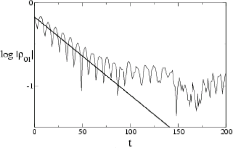
Figure 1: Dephasing of the spin system for $K=8$, $\epsilon=\epsilon_{c}/\hbar=0.3$, $\delta=0.2$, $\hbar=7.67\times 10^{-4}$, and initial spin state $|\psi_{s}\rangle=(|0\rangle+2|1\rangle)/\sqrt{5}$. The straight line fit gives $|\rho_{01}|=a\exp(-\Gamma_{2}t)$, with $a=0.40$ and $\Gamma_{2}=2.17\times 10^{-2}$. Here and in the following figures the logarithms are decimal.

The dependence of the decay rate $\Gamma_{2}$ on the coupling strength $\epsilon=\epsilon_{c}/\hbar$ is given in Fig. 2, for different values of the effective Planck constant $\hbar$. For weak coupling $\epsilon\ll 1$, we have in average

$$\Gamma_{2}\approx\epsilon^{2}/2,$$ (4)

in agreement with the expectations of the Fermi golden rule. For $\epsilon>1$, the dephasing rate saturates to an $\epsilon$-independent value. The discussion of the strong coupling regime is postponed to the end of this section.

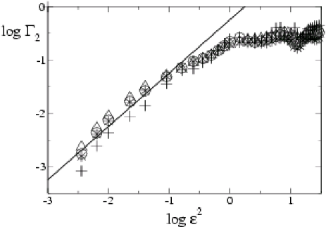
Figure 2: Dependence of dephasing rate $\Gamma_{2}$ on $\epsilon^{2}$ for $\delta=0.1$, $\hbar=4.91\times 10^{-2}$ (plus), $\hbar=1.23\times 10^{-2}$ (triangles), $\hbar=3.07\times 10^{-3}$ (circles), and $\hbar=7.67\times 10^{-4}$ (stars). The initial state and $K$ are the same as in Fig. 1. The straight line shows the average fit $\Gamma_{2}=A\epsilon^{2}$, with $A=0.57$.

As we have seen in Fig. 1, at long times $\rho_{01}(t)$ oscillates around a residual value $\rho_{\rm res}$. In Fig. 3, we show the dependence of $\rho_{\rm res}$ on the overall size $N=N_{d}N_{s}$ of the Hilbert space, where $N_{d}$ and $N_{s}=2$ are the dimensions of the Hilbert spaces for the detector and the spin, respectively. We can see that

$$\rho_{res}\propto 1/\sqrt{N},$$ (5)

as expected from the following simple statistical estimation. We assume that at long times the overall wave function is ergodic, that is,

$$|\Psi(t)\rangle=\sum_{i=0}^{1}\sum_{n=1}^{N_{d}}c_{in}(t)|i\rangle|n\rangle,$$ (6)

where the coefficients $c_{in}(t)$ have amplitudes $\sim 1/\sqrt{N}$ (to assure the wave function normalization) and random phases. Therefore, $\rho_{01}(t)=\sum_{n}c_{0n}c_{1n}^{\star}\sim 1/\sqrt{N}$ (sum of $N/2$ terms of amplitude $\sim 1/N$ with random phases).

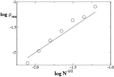
Figure 3: Dependence of $\rho_{\rm res}$ (obtained after averaging $|\rho_{01}(t)|$ over the time interval $500\leq t\leq 2000$) on the size $N$ of the overall Hilbert space. Parameter values are the same as in Fig. 1. The straight line gives $\rho_{\rm res}=1/\sqrt{N}$.

The relaxation of the diagonal component $\rho_{11}(t)$ to the asymptotic value $\rho_{11}=\frac{1}{2}$ is shown in Fig. 4 fluctuations . It can be seen that the population relaxation is exponential, with rate $\Gamma_{1}$. Indeed, the evolution in time of $\rho_{11}(t)-\frac{1}{2}$ is well fitted by the curve $a\sin(bt+\phi)\exp(-\Gamma_{1}t)$, with $b=0.404\approx 2\delta=0.4$ frequency of the free-qubit oscillations and $\Gamma_{1}=4.36\times 10^{-2}$. This fit allows us to extract the relaxation time scale $T_{1}=1/\Gamma_{1}=22.9$.

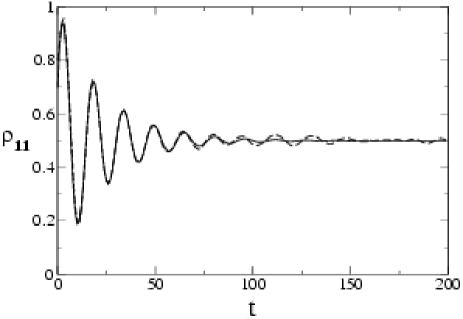
Figure 4: Population relaxation, that is, evolution in time of $\rho_{11}$ (solid curve). Parameter values are as in Fig. 1. The dashed curve shows the fit $\rho_{11}=\frac{1}{2}+a\sin(bt+\phi)\exp(-\Gamma_{1}t)$, with $a=0.5$, $b=0.404$, $\phi=0.405$ and $\Gamma_{1}=4.36\times 10^{-2}$.

The dependence of the relaxation rate $\Gamma_{1}$ on the coupling strength $\epsilon$ is shown in Fig. 5. At small $\epsilon$, the behavior of the relaxation rate is similar to that of the dephasing rate: we have

$$\Gamma_{1}\approx\Gamma_{2}\approx\epsilon^{2}/2.$$ (7)

Moreover, the relaxation rate exhibits an interesting non monotonous behavior: it has a maximum at $\Gamma_{1}\sim\delta$ and then decays when increasing $\epsilon$. This phenomenon is a manifestation of the quantum Zeno effect sudarshan ; raizen3 : repeated measurements performed by the environment (the detector) prevent the system from relaxing. In the Zeno regime, the stronger the dephasing, the slower the relaxation. In our model, this is true in a rather broad range of $\epsilon$, that is $\sqrt{\delta}\ll\epsilon<1$ (see Appendix B). In the case of Ohmic dissipation one expects schon ; schon2

$$\Gamma_{1}\sim\delta^{2}/\Gamma_{2}\sim\delta^{2}/\epsilon^{2}.$$ (8)

This is in a good agreement with our numerical data, shown in Fig. 5. In the same figure, we compare these data with the theoretical curve $\Gamma_{1}=B/\epsilon^{2}$, with the fitting constant $B=2.7\times 10^{-2}$ (note that here $\delta^{2}=10^{-2}$). For strong interactions $\epsilon>1$ the relaxation rate exhibits an oscillating behavior.

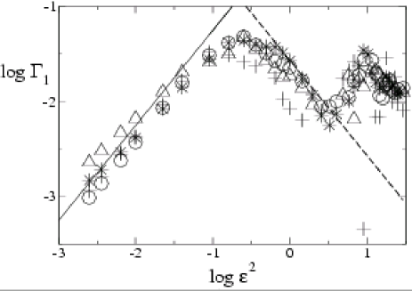
Figure 5: Dependence of the relaxation rate $\Gamma_{1}$ on the coupling strength $\epsilon$, at $\delta=0.1,K=8$, $\hbar=4.91\times 10^{-2}$ (plus), $\hbar=1.23\times 10^{-2}$ (triangles), $\hbar=3.07\times 10^{-3}$ (circles), and $\hbar=7.67\times 10^{-4}$ (stars). The initial state of the qubit is $|\psi_{s}\rangle=(|0\rangle+2|1\rangle)/\sqrt{5}$. The straight lines show $\Gamma_{1}=A\epsilon^{2}$, with $A=0.56$ (solid line) and $\Gamma_{1}=B/\epsilon^{2}$ with $B/\delta^{2}=2.7$ (dashed line).

It is interesting to compare the results obtained from our deterministic detector model with those of a quantum map derived for the system density matrix in the frame of the quantum operations formalism.

The evolution in one period of time of the system density matrix can most conveniently be written in the Bloch sphere representation, in which the coordinates $x$, $y$, and $z$ are related to the matrix elements of ${\rho}$ as follows: $\rho_{11}=\frac{1}{2}(1-z)$ and $\rho_{01}=\frac{1}{2}(x-iy)$. The free evolution between two consecutive kicks is ruled by the free Hamiltonian $\hat{H}_{s}$, that is,

$$\tilde{\rho}=e^{-i\delta\sigma_{x}}\rho e^{i\delta\sigma_{x}}.$$ (9)

From this equation we obtain

$$\left\{\begin{array}[]{l}\tilde{x}=x,\\ \tilde{y}=\cos(2\delta)y-\sin(2\delta)z,\\ \tilde{z}=\sin(2\delta)y+\cos(2\delta)z,\end{array}\right.$$ (10)

the coordinates $\tilde{x},\tilde{y},\tilde{z}$ corresponding to the density matrix $\tilde{\rho}$.

We model the effect of the interaction with the detector as a phase kick. That is to say, we assume that in the interaction Hamiltonian of Eq. (1) the angle $\theta$ is drawn from a random uniform distribution in $[0,2\pi]$. Therefore, the density matrix $\bar{\rho}$, obtained after averaging over $\theta$, is given by

$$\bar{\rho}=\frac{1}{2\pi}\int_{0}^{2\pi}d\theta R(\theta)\tilde{\rho}R^{\dagger}(\theta),$$ (11)

where

$$R(\theta)=\left[\begin{array}[]{cc}e^{-i\epsilon\cos\theta}&0\\ 0&e^{i\epsilon\cos\theta}\end{array}\right].$$ (12)

For $\epsilon\ll 1$, we obtain

$$R(\theta)\approx I-i\epsilon\cos(\theta)\sigma_{z}-\frac{\epsilon^{2}}{2}\cos^{2}(\theta)I.$$ (13)

Using this approximation, we end up with the map

$$\begin{array}[]{c}{\displaystyle\bar{\rho}=\tilde{\rho}+\epsilon^{2}\sigma_{z}\tilde{\rho}\sigma_{z}<\cos^{2}\theta>-\epsilon^{2}<\cos^{2}\theta>\tilde{\rho}}\\ {\displaystyle=\left(1-\frac{\epsilon^{2}}{2}\right)\tilde{\rho}+\frac{\epsilon^{2}}{2}\sigma_{z}\tilde{\rho}\sigma_{z}},\end{array}$$ (14)

where in the random phase approximation we take $<\cos^{2}\theta>=\frac{1}{2\pi}\int_{0}^{2\pi}d\theta\cos^{2}\theta=\frac{1}{2}$. This map is known as the phase damping noise channel chuang ; cpos .

Map (14) can be written in the Bloch sphere coordinates as follows:

$$\left\{\begin{array}[]{l}\bar{x}=(1-\epsilon^{2})\tilde{x}=(1-\epsilon^{2})x,\\ \bar{y}=(1-\epsilon^{2})\tilde{y}=(1-\epsilon^{2})[\cos(2\delta)y-\sin(2\delta)z],\\ \bar{z}=\tilde{z}=\sin(2\delta)y+\cos(2\delta)z,\end{array}\right.$$ (15)

where the coordinates $\bar{x},\bar{y},\bar{z}$ correspond to $\bar{\rho}$. An alternative derivation of map (15), based on the master equation approach, is provided in Appendix A.

This map gives the evolution of the Bloch sphere coordinates in one kick and can be iterated. From the values of the coordinates $x$, $y$, and $z$ after $t$ map steps we can obtain $\rho_{01}$ and $\rho_{11}$ at time $t$. An example of numerical solution of map (15) is shown in Fig. 6. The exponential decay of $\rho_{01}$ and the exponential relaxation of $\rho_{11}$ to the steady state value $\frac{1}{2}$ can be clearly seen. Similarly to Fig. 1 and Fig. 4, we also have oscillations with the Rabi frequency. We also checked that the relaxation rates $\Gamma_{1}$ and $\Gamma_{2}$ are both proportional to $\epsilon^{2}$. More precisely, the numerical data for the model (15) give $\Gamma_{1}\approx\Gamma_{2}\approx 0.53\epsilon^{2}$. These rates are in good agreement with those from the numerical data obtained for the whole system (qubit plus detector) and shown in Fig. 2 and Fig. 5. Therefore, it is noteworthy that our fully deterministic dynamical model can reproduce the main features of the single-qubit decoherence due to a heat bath. Our results are also in agreement with the analytical solution obtained in the continuous time limit and described in Appendix B.

Figure 6: Dephasing and relaxation in the phase damping map (15). Main figure: time dependence of $|\rho_{01}|$ for $\epsilon=0.225$ and other parameter values as in Fig. 1. The straight line fit gives the exponential decay $|\rho_{01}|=a\exp(-\Gamma_{2}t)$, with $a=0.31$ and $\Gamma_{2}=2.77\times 10^{-2}=0.55\epsilon^{2}$. Inset: same as in the main figure but for $\rho_{11}$. The behavior of $\rho_{11}$ (dots) is very well reproduced by the fit $\rho_{11}=\frac{1}{2}+a\sin(bt+\phi)\exp(-\Gamma_{1}t)$, with $a=0.3$, $b=0.4$, $\phi=1.52$ and $\Gamma_{1}=2.30\times 10^{-2}=0.45\epsilon^{2}$ (solid curve).

To close this section, we discuss the case in which the coupling strength is classically strong, namely $\epsilon_{c}\sim 1$, corresponding to $\epsilon\gg 1$ for a quasi-classical detector ($\hbar\ll 1$). As shown in Fig. 7, the dephasing rate is given by the Lyapunov exponent $\lambda$ of the underlying classical chaotic dynamics of the kicked rotator. We point out that, in this regime, the dephasing rate is independent of the interaction strength. This result can be understood as follows. Assuming that the period of the free oscillations of the system is much larger than the dephasing time, namely $1/\delta\gg\lambda$, we have

$$\rho_{01}(t)\approx\rho_{01}(0)\langle\psi_{d}|(\hat{U}_{d,+}^{\dagger})^{t}(\hat{U}_{d,-})^{t}|\psi_{d}\rangle,$$ (16)

where $\hat{U}_{d,+}$ and $\hat{U}_{d,-}$ are the one-kick evolution operators for the detector when the effective kicking strengths are $K_{\rm eff}=K_{+}=K+\epsilon_{c}$ and $K_{\rm eff}=K_{-}=K-\epsilon_{c}$, respectively rho11 . For $K_{\rm eff}=K_{-}$, the initial Gaussian wave packet is centered at a stable fixed point and therefore, for short times, $(\hat{U}_{d,-})^{t}|\psi_{d}\rangle\approx|\psi_{d}\rangle$. On the other hand, the same fixed point is unstable for $K_{\rm eff}=K_{+}$. Therefore, in the quasi-classical regime and for strong enough perturbations the wave packet spreads along the direction of instability for the classical motion, with rate given by the Lyapunov exponent. We note that this phenomenon is closely related to the Lyapunov decay of the fidelity of quantum motion in chaotic systems jalabert ; jacquod ; benenti ; prosen ; zurek . Indeed, Eq. (16) shows that $\rho_{01}(t)$ is proportional to the fidelity amplitude $f(t)=\langle\psi_{d}|(\hat{U}_{d,+}^{\dagger})^{t}(\hat{U}_{d,-})^{t}|\psi_{d}\rangle$. This quantity measures the stability of quantum motion under perturbations. More precisely, $f(t)$ is the overlap of two states which, starting from the same initial conditions, evolve under two slightly different Hamiltonians. The above discussion shows that the fidelity decay has an interesting interpretation in terms of dephasing of an appropriate two-level systems.

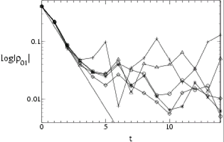
Figure 7: Time dependence of $|\rho_{01}|$ for $K=4.5$, $\epsilon_{c}\equiv\epsilon 2\pi/2^{n-1}=0.8$, and $\delta=0.01$. The initial state of the qubit is $|\psi_{s}\rangle=(|0\rangle+2|1\rangle)/\sqrt{5}$, the initial detector state is a Gaussian wave packet with area size $\hbar$ centered at $p=0$, $\theta=\pi$. Data are shown for $\hbar=4.91\times 10^{-2}$ (plus), $\hbar=1.23\times 10^{-2}$ (triangles), $\hbar=3.07\times 10^{-3}$ (circles), $\hbar=7.67\times 10^{-4}$ (stars), and $\hbar=1.92\times 10^{-4}$ (diamonds). The straight line represents the exponential decay with rate given by the Lyapunov exponent $\lambda\approx\ln(K/2)=0.81$ chirikov79 .

IV Detector model

In this section, we study the efficiency of the detector in the regimes of weak and strong system-detector coupling.

Let us first discuss the strong measurement case with $\epsilon_{c}$ large $\epsilon_{c}\sim 1$. In this case, the effective coupling strength $K_{\rm eff}=K+\epsilon_{c}\sigma_{z}$ significantly depends on the up or down state of the spin system. Therefore, it is easy to find regimes in which the response of the detector clearly depends on the state of the system. An example is shown in Figs. 8-9. In these figures, we have $K=4.5$, while $K_{\rm eff}=K-\epsilon_{c}=3.8$ when the rotator is coupled to a down spin ($\sigma_{z}=-1$) and $K_{\rm eff}=K+\epsilon_{c}=5.2$ when the rotator is coupled to an up spin ($\sigma_{z}=+1$). The initial Gaussian packet is centered at the fixed point $p=0$, $\theta=\pi$. A linear stability analysis of the classical dynamics of the kicked rotator shows that this fixed point is stable for $0\leq K\leq 4$ and unstable for $K>4$ and $K<0$. Therefore, in the case of coupling to a down spin, the fixed point is stable ($K_{\rm eff}<4$), while the same point is unstable when the detector is coupled to an up spin ($K_{\rm eff}>4$). In Fig. 8, we see that, if the qubit is in its up state, the Husimi function is spread in the phase space after $t=20$ kicks (left plot) husimi . On the contrary, if the qubit is in its down state, the Husimi function is localized around the stable fixed point at $t=20$ (right plot). The difference between the Husimi distributions in these two cases is evident and leads to measurable effects. Indeed, as shown in Fig. 9, the values of the second moment $<p^{2}>$ are very different at short times for up and down spins.

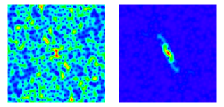
Figure 8: (Color online) Husimi function in action-angle variables $(p,\theta)$ for the detector, with $-\pi\leq p<\pi$ (vertical axis) and $0\leq\theta<2\pi$ (horizontal axis) for the kicked rotator coupled to up spin (left) and down spin (right), at $K=4.5$, $\epsilon_{c}=0.8$, $\delta=0.1$, $\hbar=1.23\times 10^{-2}$, $t=20$. The initial states of the kicked rotator and the qubit are a Gaussian packet centered at the fixed point $p=0$, $\theta=\pi$ and $|\psi_{s}\rangle=(|0\rangle+|1\rangle)/\sqrt{2}$. Color represents the density from blue/black (minimal value) to red/gray (maximal value).

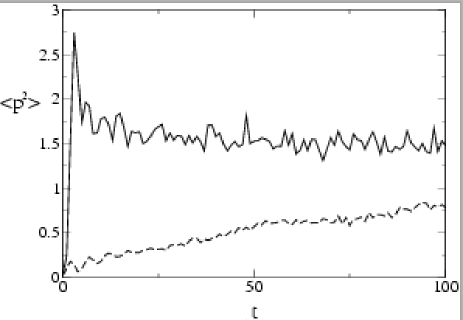
Figure 9: Time dependence of $\langle p^{2}\rangle$ for up spin (curve) and down spin (dashed curve). Parameter values are the same as in Fig.8.

It is interesting to discuss the case of weak system-detector coupling with $\epsilon\sim 1$, $\epsilon_{c}=\epsilon\hbar\ll 1$. In the chaotic regime for the kicked rotator the Husimi function exhibits hypersensitivity to perturbations simone . Indeed, as shown in Fig. 10, we have markedly different Husimi functions when the detector is coupled to up or down spin. In the case of Fig. 10, we have $\epsilon=0.4$ and $\hbar=1.23\times 10^{-2}$, corresponding to $\epsilon_{c}=4.91\times 10^{-3}\ll 1$. However, it is unclear how to extract measurable information from this difference. Indeed, it is reasonable to assume that only the coarse graining properties of the semi-classical detector are accessible, the size of the coarse graining being much larger than the Planck cell. The difficulty to distinguish the left and right Husimi plots of Fig. 10 after coarse graining is illustrated in Fig. 11. In this latter figure we compute the integral $W_{D}$ of the Husimi distribution over a box of size $2.53\times 10^{-1}\gg\hbar=1.23\times 10^{-2}$, centered, as the initial wave packet, at $p=0$, $\theta=\pi$. The evolution in time of $W_{D}$ is shown for different but small coupling strengths ($\epsilon_{c}\ll 1$). It is clear that the evolutions of $W_{D}(t)$ for up and down spin states can be hardly distinguished.

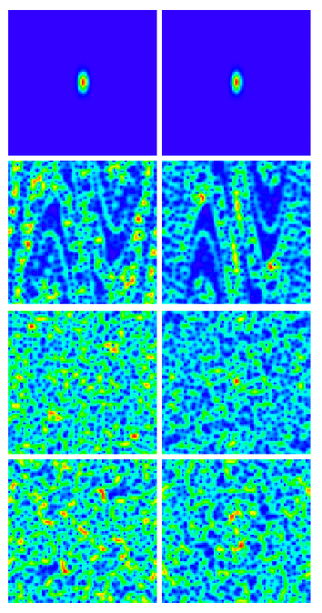
Figure 10: (Color online) Hypersensitivity of the Husimi function on the spin value for $K=8$, $\epsilon=0.4$, $\delta=0.2$, and $\hbar=1.23\times 10^{-2}$. From top to bottom $t=0$, $4$, $8$, $12$. The left plots are for up spin, the right ones for down spin. The initial states of the kicked rotator and of the qubit are a Gaussian packet centered at the fixed point $p=0$, $\theta=\pi$ and $|\psi_{s}\rangle=(|0\rangle+|1\rangle)/\sqrt{2}$. The color code is as in Fig. 8.

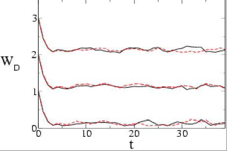
Figure 11: (Color online) Integral $W_{D}$ of the Husimi distribution over a square box of size $2.53\times 10^{-1}\gg\hbar=1.23\times 10^{-2}$, centered at $p=0$, $\theta=\pi$, for spin up (dashed red/gray curve) and spin down (solid black curve) states. From top to bottom: ($\epsilon=0.4$, $\delta=0.0$), ($\epsilon=0.2$, $\delta=0.2$), and ($\epsilon=0.4$, $\delta=0.2$). The initial state of the detector and the other parameter values are as in Fig. 10. The top and middle curves are shifted in the $y$-axis direction by $+2$ and $+1$, respectively.

V Conclusions

In this paper we have proposed and studied a deterministic model of quasi-classical detector coupled to a single-qubit system. Our results show that the detector introduces dynamical decoherence in the system. Moreover, we have shown that an efficient measurement is possible in the case of strong system-detector coupling. In the case of weak coupling, the chaotic dynamics of the detector is still hypersensitive to the state of the qubit but it is unclear how to detect the up/down states in a coarse graining measurement. It is an interesting question whether this conclusion remains valid when the unavoidable coupling of the detector with a dissipative environment is taken into account.

We thank the IDRIS in Orsay and CalMiP in Toulouse for access to their supercomputers. This work was supported in part by the project EDIQIP of the IST-FET program of the EC.

Appendix A Master equation

In this Appendix, we provide an alternative derivation of the phase damping map (15), based on the master equation approach. For this purpose, we start from the overall Hamiltonian of Eq. (1) and make the usual Born and Markov approximations. That is to say, we assume that the detector’s dynamics is practically unaffected by the interaction with the qubit and that any effect the qubit has on the detector is limited to a time scale much shorter than the time scales of interest for the dynamics of the qubit. The first condition is fulfilled in the case of weak coupling, $\epsilon\ll 1$, the second is satisfied due to the fast decay of correlations for the detector in the chaotic regime (here we assume that $\delta\ll 1$ and that correlations decay in a few kicks). Under these assumptions, we can derive master the following master equation:

$$\begin{array}[]{c}\displaystyle{\frac{d\hat{\rho}}{dt}=-i[\hat{H}_{s},\hat{\rho}]+\frac{\gamma}{2}\left([\hat{\sigma}_{z},\hat{\rho}\hat{\sigma}_{z}]+[\hat{\sigma}_{z}\hat{\rho},\hat{\sigma}_{z}]\right)}\\ \displaystyle{=-i[\hat{H}_{s},\hat{\rho}]+\frac{\epsilon_{c}^{2}}{2}(\hat{\sigma}_{z}\hat{\rho}\hat{\sigma}_{z}-\hat{\rho})\sum_{m}\delta(t-m),}\end{array}$$ (17)

where we have used

$$\begin{array}[]{c}{\displaystyle\gamma=\epsilon_{c}^{2}{\rm Tr}_{d}[\cos^{2}(\tilde{\theta})\tilde{\rho}_{d}]\sum_{m}\delta(t-m)}\\ {\displaystyle=\frac{\epsilon_{c}^{2}}{2}\sum_{m}\delta(t-m).}\end{array}$$ (18)

Here $\tilde{\rho}_{d}$ is the detector’s density matrix and the tilde denotes the fact that we are using the interaction picture (that is, the time evolution of the operators with a tilde is ruled by the detector’s Hamiltonian $\hat{H}_{d}$). Assuming that the density matrix $\tilde{\rho}_{d}$ corresponds to a uniform distribution in the $\theta$ variable, we obtain ${\rm Tr}_{d}[\cos^{2}(\tilde{\theta})\tilde{\rho}_{d}]\approx\frac{1}{2\pi}\int_{0}^{2\pi}d\theta\cos^{2}\theta=\frac{1}{2}$. The integration of the master equation (17) in one time step leads to the phase damping map (15).

Appendix B Continuous model

The continuous version of the phase damping map (15) is

$$\left\{\begin{array}[]{l}\dot{x}=-\epsilon^{2}x,\\ \dot{y}=-\epsilon^{2}y-2\delta z,\\ \dot{z}=2\delta y.\end{array}\right.$$ (19)

The solution for $x(t)$ is a simple decay with the rate $\Gamma=\epsilon^{2}$:

$$x(t)=x(0)e^{-\Gamma t}.$$ (20)

The solution for $y(t)$ and $z(t)$ reads as follows:

$$\left\{\begin{array}[]{l}y(t)=[a\sin(\omega t)+b\cos(\omega t)]e^{-\Gamma t/2},\\ z(t)=[c\sin(\omega t)+d\cos(\omega t)]e^{-\Gamma t/2},\end{array}\right.$$ (21)

where

$$\omega=\sqrt{4\delta^{2}-\frac{\Gamma^{2}}{4}}$$ (22)

and the coefficients $a,b,c,d$ can be expressed as a function of the initial conditions $y(0),z(0)$. Therefore, for $\epsilon\ll 2\sqrt{\delta}$, in the $\hat{\sigma}_{z}$-basis both the diagonal and the off-diagonal elements of the density matrix decay as $\frac{\Gamma}{2}$, in agreement with our numerical data shown in Sec. III. Indeed, we have at large times $|\rho_{11}-\frac{1}{2}|=|z|\sim\exp(-\Gamma t/2)$ and $|\rho_{01}|=\frac{1}{2}(x^{2}+y^{2})^{1/2}\sim|y|\sim\exp(-\Gamma t/2)$.

When the coupling to the detector becomes strong, so that $\Gamma>4\delta$, then the oscillations in $y(t)$ and $z(t)$ turn into decay with two characteristic rates:

$$\Gamma_{\pm}=\frac{\Gamma}{2}\pm\sqrt{\frac{\Gamma^{2}}{4}-4\delta^{2}}\;.$$ (23)

The smallest rate ($\Gamma_{-}$) describes the quantum Zeno effect. For $\Gamma\gg 4\delta$ we obtain $\Gamma_{-}\simeq 4\delta^{2}/\Gamma$, in agreement with our numerical results shown in Fig. 5.

It is important to remark that in the basis of the eigenstates of the Hamiltonian $\hat{H}_{s}$ one can recover the relaxation and decoherence time scales usually discussed in the literature. In this basis $x$ describes the deviation of the diagonal elements of the density matrix from $1/2$, while $y$ and $z$ give the decay of the real and imaginary part of the off-diagonal matrix elements. Therefore, for $\epsilon<2\sqrt{\delta}$ the diagonal elements decay with rate $\Gamma$ and the off-diagonal elements with rate $\Gamma/2$.

References

- (1) V. B. Braginsky and F. Ya. Khalili, Quantum Measurement (Cambridge Univ. Press, 1992).
- (2) D. Giulini, E. Joos, C. Kiefer, J. Kupsch, I.-O. Stamatescu, and H.-D. Zeh, Decoherence and the Appearance of a Classical World in Quantum Theory (Springer, Berlin, 1996).
- (3) M. Namiki, S. Pascazio, and H. Nakazato, Decoherence and Quantum Measurements (World Scientific, Singapore, 1997).
- (4) F. Schmidt-Kaler, H. Häffner, M. Riebe, S. Gulde, G.P.T. Lancaster, T. Deuschle, C. Becher, C.F. Roos, J. Eschner, and R. Blatt, Nature 422, 408 (2003); M. Riebe, H. Häffner, C.F. Roos, W. Hänsel, J. Benhelm, G.P.T. Lancaster, T.W. Körber, C. Becher, F. Schmidt-Kaler, D.F.V. James, and R. Blatt, Nature 429, 734 (2004).
- (5) M.D. Barrett, J. Chiaverini, T. Schaetz, J. Britton, W.M. Itano, J.D. Jost, E. Knill, C. Langer, D. Leibfried, R. Ozeri, and D.J. Wineland, Nature 429, 737 (2004).
- (6) S.A. Gurvitz, Phys. Rev. B 56, 15215 (1997).
- (7) A.N. Korotkov, Phys. Rev. B 63, 115403 (2001).
- (8) A.N. Korotkov and D.V. Averin, Phys. Rev. B 64, 165310 (2001).
- (9) H.-S. Goan, G.J. Milburn, H.M. Wiseman, and H.B.Sun, Phys. Rev. B 63, 125326 (2001).
- (10) D. Mozyrsky, L. Fedichkin, S.A. Gurvitz, and G.P. Berman, Phys. Rev. B 66, R161313 (2002).
- (11) L.N. Bulaevskii and G. Ortiz, Phys. Rev. Lett. 90, 040401 (2003).
- (12) W. Mao, D.V. Averin, F. Plastina, and R. Fazio, cond-mat/0408471.
- (13) Y. Makhlin, G. Schön, and A. Shnirman, Rev. Mod. Phys. 73, 357 (2001).
- (14) D. Vion, A. Aassime, A. Cottet, P. Joyez, H. Pothier, C. Urbina, D. Esteve, and M.H. Devoret, Science 296, 886 (2002).
- (15) I. Chiorescu, Y. Nakamura, C.J.P.M. Harmans, and J.E. Mooij, Science 299, 1869 (2003).
- (16) O. Astafiev, Yu. A. Pashkin, T. Yamamoto, Y. Nakamura, and J.S. Tsai, Phys. Rev. B 69, 180507(R) (2004).
- (17) E. Il’ichev, N. Oukhanski, A. Izmalkov, Th. Wagner, M. Grajcar, H.-G. Meyer, A.Yu. Smirnov, A. Maassen van den Brink, M.H.S. Amin, and A.M. Zagoskin, Phys. Rev. Lett. 91, 097906 (2003).
- (18) For a review see, e.g., B. V. Chirikov, in Chaos and Quantum Physics, Les Houches Lecture Series 52 Eds. M.-J. Giannoni, A.Voros, and J. Zinn-Justin (North-Holland, Amsterdam, 1991), p.443; F.M. Izrailev, Phys. Rep. 196, 299 (1990).
- (19) D.A. Steck, W.H. Oskay, and M.G. Raizen, Science 293, 274 (2001).
- (20) W.K. Hensinger, H. Haffner, A. Browaeys, N.R. Heckenberg, K. Helmerson, C. McKenzie, G.J. Milburn, W.D. Phillips, S.R. Rolston, H. Rubinsztein-Dunlop, and B. Upcroft, Nature 412, 52 (2001).
- (21) F.L. Moore, J.C. Robinson, C.F. Bharucha, B. Sundaram, and M.G. Raizen, Phys. Rev. Lett. 75, 4598 (1995).
- (22) H. Ammann, R. Gray, I. Shvarchuck, and N. Christensen, Phys. Rev. Lett. 80, 4111 (1998).
- (23) J. Ringot, P. Szriftgiser, J.C. Garreau, and D. Delande, Phys. Rev. Lett. 85, 2741 (2000).
- (24) S. Schlunk, M.B. d’Arcy, S.A. Gardiner, D. Cassettari, R.M. Godun, and G.S. Summy, Phys. Rev. Lett. 90, 054101 (2003).
- (25) Z.-Y. Ma, M.B. d’Arcy, and S.A. Gardiner, Phys. Rev. Lett. 93, 164101 (2004).
- (26) Here we do not discuss quantum nondemolition measurements, i.e., when measuring an observable which commutes with the Hamiltonian and is, thus, conserved. In this special case, it is possible to measure the system without perturbing it. See, e.g., D.V. Averin, Phys. Rev. Lett. 88, 207901 (2002), and references therein.
- (27) Chaotic baths are actively discussed in the literature. See, e.g., R. Blume-Kohout and W.H. Zurek, Phys. Rev. A 68, 032104 (2003) and J. Lages, V.V. Dobrovitski, and B.N. Harmon, quant-ph/0406001.
- (28) B. V. Chirikov, Phys. Rep. 52, 263 (1979).
- (29) S.A. Gardiner, J.I. Cirac, and P. Zoller, Phys. Rev. Lett. 79, 4790 (1997).
- (30) A. Peres, Phys. Rev. A 30, 1610 (1984).
- (31) R.A. Jalabert and H.M. Pastawski, Phys. Rev. Lett. 86, 2490 (2001).
- (32) Ph. Jacquod, P.G. Silvestrov, and C.W.J. Beenakker, Phys. Rev. E 64, 055203(R) (2001).
- (33) G. Benenti and G. Casati, Phys. Rev. E 65, 066205 (2002).
- (34) T. Prosen and M. Žnidarič, J. Phys. A 35, 1455 (2002).
- (35) F.M. Cucchietti, D.A.R. Dalvit, J.P. Paz, and W.H. Zurek, Phys. Rev. Lett. 91, 210403 (2003).
- (36) We have checked that the times and (measured in number of kicks) do not significantly depend on , provided that .
- (37) Similarly to the off-diagonal matrix elements, fluctuations around the value remain at long times due to the finite size of the overall system.
- (38) B. Misra and E.C.G. Sudarshan, J. Math. Phys. 18, 756 (1977).
- (39) M.C. Fischer, B. Gutiérrez-Medina, and M.G. Raizen, Phys. Rev. Lett. 87, 040402 (2001).
- (40) Y. Makhlin, G. Schön, and A. Shnirman, cond-mat/0309049, in New Directions in Mesoscopic Physics (towards Nanoscience), eds. R. Fazio, V.F. Gantmakher, and Y. Imry, Kluwer (2003), p. 197, Proceedings of the NATO-ASI, Erice, Italy, July 20 - August 1, 2002.
- (41) See, e.g., M.A. Nielsen and I.L. Chuang, Quantum computation and quantum information (Cambridge University Press, Cambridge, 2000).
- (42) Map (14) is completely positive and can be written in the Kraus form as follows: , with the Kraus operators and satisfying the condition .
- (43) The derivation of the master equation from a system plus bath Hamiltonian is described, for instance, in C.W. Gardiner and P. Zoller, Quantum Noise, Springer-Verlag (2000), chap. 5.
- (44) The same argument tells us that, at short times, populations essentially do not decay, that is, for .
- (45) The computation of Husimi functions is described in S.-J. Chang and K.-J. Shi, Phys. Rev. A 34, 7 (1986).
- (46) G. Benenti, G. Casati, S. Montangero, and D.L. Shepelyansky, Eur. Phys. J. D 20, 293 (2002).