Thermal Entanglement of bosonic modes
M. Asoudeh,

Department of Physics, Sharif University of Technology,

P.O. Box 11365-9161,

Tehran, Iran

We study the change of entanglement under general linear transformation of modes in a bosonic system and determine the conditions under which entanglement can be generated under such transformations. As an example we consider the thermal entanglement between the vibrational modes of two coupled oscillators and determine the temperature above which quantum correlations are destroyed by thermal fluctuations.

1 Introduction

Consider two ions in an ion trap, or two atoms in a solid vibrating around their equilibrium positions. We ask how much pure quantum correlation or entanglement exists between the vibrational modes of these two ions or atoms at a given temperature? How much we can raise the temperature before the quantum correlation between the ions is destroyed? In a more general context, we can ask the degree of entanglement of two bosonic modes in a many body system. This property known as thermal entanglement has been intensively studied mostly for the spin degrees of freedom of atoms or ions in the past two or three years [1, 2, 3]. The reason for this restriction has been threefold. The first is that a calculable measure of entanglement when the two systems are in a mixed state has been known only for two dimensional systems [4]. The second reason has been obviously the interest in two dimensional systems as representatives of qubits in quantum computers [5]. The third is that spin systems are the prototype of interacting many body localized fermions and it has been desirable to see what happens to entanglement when a spin system undergoes quantum phase transition [6].
While the pursuit of this problem for intermediate dimensions has been impossible (for the lack of a measure of entanglement) or of little interest, all the above three motivations exist also for the other extreme of dimensionality, namely systems with continuous degrees of freedom. First, for a class of states called symmetric Gaussian states, a closed formula exist for their entanglement of formation[7], second, systems of continuous degrees of freedom are of wide interest as candidates for the implementation of quantum computing [8] and third, in condensed matter systems, the continuous degrees of freedom like the vibrational modes of localized atoms in a crystal or the bosonic modes of a system of identical particles can also be entangled. The same phenomenon is of interest in bosonic field theories [13].
When dealing with systems of identical particles, it is the modes and not the particles which should be treated as subsystems [9] and one can quantify the entanglement of these subsystems in a second quantized approach[9, 10, 11, 12, 13]. In this case entanglement changes by redefining the modes, a non-local operation on subsystems.
In this paper we study a system composed of identical spinless bosons subject to a free quadratic hamiltonian and study the thermal entanglement properties of different arbitrary modes of this system. This problem will also be of relevance when we want to understand how thermal fluctuations will affect the efficiency of protocols based on gaussian states [14].
So we consider a hamiltonian of the form

$$H=\sum_{\alpha=1}^{L}\omega_{\alpha}b^{\dagger}_{\alpha}b_{\alpha}$$ (1)

with $[b_{\alpha},b^{\dagger}_{\beta}]=\delta_{\alpha\beta}$ and a general linear mode transformation

$$a_{i} = \sum_{\alpha=1}^{L}(S_{i\alpha}^{*}b_{\alpha}+T_{i\alpha}b_{\alpha}^{\dagger}),$$ (2)

$${a_{i}}^{\dagger} = \sum_{\alpha=1}^{L}(S_{i\alpha}b_{\alpha}^{\dagger}+T_{i\alpha}^{*}b_{\alpha}).$$ (3)

To ensure the correct commutation relations between the new modes, the matrices $S$ and $T$ should satisfy:

$$[S^{\dagger},T]=0\ ,\ \ S^{\dagger}S-TT^{\dagger}=I.$$ (4)

We ask how much entanglement exists between modes $k$ and $l$. This requires that we calculate the reduced density matrix of these two modes, $\rho_{kl}:=tr_{\widehat{k,l}}(\rho_{{\rm{th}}})$ where $\rho_{{\rm{th}}}=\frac{1}{Z}e^{-\beta H}$, $Z=tr(e^{-\beta H})$, and $\widehat{k,l}$ means that the modes $k$ and $l$ are excluded when taking the trace.
We will show that the reduced density matrix of any two modes, is always a gaussian state(?). We obtain the condition under which the transformations (2) can not produce entanglement. We then consider an example which is a prototype of a wider class and calculate exactly the entanglement between the two modes and its dependence on temperature, specifically we obtain the threshold temperature above which quantum correlations are destroyed.
We begin by collecting the necessary ingredients about gaussian states that we need in the sequel. In the Hilbert space of two harmonic oscillators a density matrix $\rho$ is called a two mode gaussian state if its characteristic function, defined as

$$C(z_{1}^{*},z_{1},z_{2}^{*},z_{2})=tr(e^{z_{1}a_{1}^{\dagger}-z_{1}^{*}a_{1}+z_{2}a_{2}^{\dagger}-z_{2}^{*}a_{2}}\rho),$$

is a gaussian function. This can be written compactly as

$$C(z_{1}^{*},z_{1},z_{2}^{*},z_{2})=e^{-\frac{1}{2}{\bf z}^{\dagger}M{\bf z}},$$ (5)

where ${\bf z}^{\dagger}=\left(\begin{array}[]{cccc}z_{1}^{*}&z_{1}&z_{2}^{*}&z_{2}\\ \end{array}\right)$ and $M$, parameterized as

$$M=\left(\begin{array}[]{cc}{\mathbf{\alpha}}&{\mathbf{\gamma}}\\ {\mathbf{\gamma}}^{\dagger}&{\mathbf{\beta}}\\ \end{array}\right)\equiv\left(\begin{array}[]{cccc}n_{1}&m_{1}&m_{s}&m_{c}\\ m_{1}^{*}&n_{1}&m_{c}^{*}&m_{s}^{*}\\ m_{s}^{*}&m_{c}&n_{2}&m_{2}\\ m_{c}^{*}&m_{s}&m_{2}^{*}&n_{2}\\ \end{array}\right)$$ (6)

is called the covariance matrix [15].
This matrix encodes all the correlations in the form $M_{rs}=\frac{(-1)^{r+s}}{2}\langle v_{r}{v^{\dagger}}_{s}+{v^{\dagger}}_{s}v_{r}\rangle$, where $v^{\dagger}=(a_{1}^{\dagger},a_{1},a_{2}^{\dagger},a_{2})$ and $v:=(a_{1},a_{1}^{\dagger},a_{2},a_{2}^{\dagger})^{T}$.
The conditions of separability of the two modes have been studied in a number of works [16, 17]. In particular it has been shown that by a canonical transformation the covariance matrix can be put that when the covariance for a class of in which $m_{c}=m_{1}=m_{2}=0$. The conditions of separability then simplify to the following inequalities [17]:

$$n_{1}\geq\frac{1}{2}\ \ \ \ {\rm and}\ \ \ \ (n_{1}-\frac{1}{2})(n_{2}-\frac{1}{2})\geq|m_{s}|^{2}.$$ (7)

The above conditions only determine the separability of a gaussian state and not the amount of its entanglement. For a class of gaussian states invariant under the interchange of the two modes and called symmetric states, one can actually calculate in closed form the entanglement of formation [7]. The closed formula is given in terms of the covariance matrix $\Gamma$ defined as $\Gamma_{rs}=\langle\eta_{r}\eta_{s}+\eta_{s}\eta_{r}\rangle$, where $\eta:=(x_{1},p_{1},x_{2},p_{2})$ , $x_{r}:=\frac{1}{\sqrt{2}}(a_{r}+a_{r}^{\dagger})$ and $p_{r}:=\frac{i}{\sqrt{2}}(a_{r}^{\dagger}-a_{r}),\ r=1,2$. For the covariance matrix $M$ given in (6), the covariance matrix $\Gamma$ will have the form:

$$\Gamma=2\left(\begin{array}[]{cc}Q&0\\ 0&Q\\ \end{array}\right)M\left(\begin{array}[]{cc}Q^{\prime}&0\\ 0&Q^{\prime}\\ \end{array}\ \right),$$ (8)

where $Q=\frac{1}{\sqrt{2}}\left(\begin{array}[]{cc}-1&1\\ i&i\\ \end{array}\right)$ and $Q^{\prime}=\frac{1}{\sqrt{2}}\left(\begin{array}[]{cc}-1&-i\\ 1&-i\\ \end{array}\right)$.
For symmetric gaussian states (those for which $\det{\mathbf{\alpha}}=\det{\mathbf{\beta}}$) one can apply local symplectic transformation [18, 19] and without changing their entanglement put their covariance matrix into the normal form

$$\Gamma=\left(\begin{array}[]{cccc}n&0&k_{x}&0\\ 0&n&0&-k_{p}\\ k_{x}&0&n&0\\ 0&-k_{p}&0&n\\ \end{array}\right),$$ (9)

where $k_{x}\geq k_{p}\geq 0$. These new parameters are derivable from the symplectic invariants of the matrix $M$:

$$n^{2}=4\det{\mathbf{\alpha}},\ \ k_{x}k_{p}=4|\det{\mathbf{\gamma}}|,$$

$$(n^{2}-k_{x}^{2})(n^{2}-k_{p}^{2})=4\det M.$$

The entanglement of formation of these symmetric states is then given by

$$E_{f}(\rho):=c_{+}\log c_{+}-c_{-}\log c_{-},$$ (10)

where $c_{\pm}=\frac{(1\pm\Delta)^{2}}{4\Delta}$, and

$$\Delta=min\left(1,\delta:=\sqrt{(n-k_{x})(n-k_{p})}\right).$$ (11)

The state is entangled only when $\Delta<1.$
Finally we note that for a state like $\rho_{\alpha}:=\frac{1}{Z}e^{-\beta\omega_{\alpha}b_{\alpha}^{\dagger}b_{\alpha}}$ where $b_{\alpha}$ and $b_{\alpha}^{\dagger}$ are the usual harmonic oscillator operators, $[b_{\alpha},b_{\alpha}^{\dagger}]=1$, and $Z=(1-e^{-\beta\omega_{\alpha}})^{-1}$, the single mode characteristic function $C_{\alpha}(z^{*},z):=tr(e^{zb^{\dagger}-z^{*}b}\rho_{\alpha})$ is found to be

$$C_{\alpha}(z^{*},z)=e^{\frac{-|z|^{2}}{2}\coth\frac{\beta\omega_{\alpha}}{2}}.$$ (12)

One way for doing this calculation is to expand the trace in the eigenstates of $b^{\dagger}b$. Then by using the properties of coherent states $|z\rangle:=e^{zb^{\dagger}}|0\rangle$, (i.e. $b|z\rangle=z|z\rangle,\langle z|\gamma\rangle=e^{z^{*}\gamma}$ and $\frac{1}{\pi}\int d\gamma d\gamma^{*}e^{-|\gamma|^{2}}|\gamma\rangle\langle\gamma|=I$), one writes

$$\langle n|e^{-z^{*}b}e^{zb^{\dagger}}|n\rangle=\frac{1}{n!}\langle-z|b^{n}{b^{\dagger}}^{n}|z\rangle$$ (13)

$$= \int d\gamma d\gamma^{*}|\gamma|^{2n}e^{-z^{*}\gamma+\gamma^{*}z-|\gamma|^{2}}.$$ (14)

By summing over $n$ and performing the resulting gaussian integration one arrives at the stated result. Also for any two commuting modes

$$C_{\alpha\beta}(z_{1}^{*},z_{1},z_{2}^{*},z_{2})=C_{\alpha}(z_{1}^{*},z_{1})C_{\beta}(z_{2}^{*},z_{2}).$$ (15)

This completes our short review of gaussian states.
We now consider our mode transformations (2). To express the covariance matrix of any two modes, say the modes $k$ and $l$ it is useful to introduce a compact notation. Let

$$|S_{k}\rangle:=\left(\begin{array}[]{c}S_{k1}\\ S_{k2}\\ \cdot\\ S_{kL}\\ \end{array}\right)\ \ ,\ \ |T_{k}\rangle:=\left(\begin{array}[]{c}T_{k1}\\ T_{k2}\\ \cdot\\ T_{kL}\\ \end{array}\right),$$ (16)

and define the positive inner product between any two such vectors as

$$\langle X|Y\rangle:=\sum_{\alpha=1}^{L}\coth\frac{\beta\omega_{\alpha}}{2}X_{\alpha}^{*}Y_{\alpha}.$$ (17)

The characteristic function of the two modes is given by

$$C_{kl}(z_{1}^{*},z_{1},z_{2}^{*},z_{2})=tr(e^{z_{1}a_{k}^{\dagger}-z_{1}^{*}a_{k}+z_{2}a_{l}^{\dagger}-z_{2}^{*}a_{l}}\otimes_{\alpha=1}^{L}\rho_{\alpha}).$$ (18)

By noting from (1) that $\rho_{\rm{th}}=\bigotimes\rho_{\alpha}$, and inserting (2) in (18), rearranging the terms in the exponential and using (12) and (15) we find

$$C_{kl}=e^{-\frac{1}{2}\sum_{\alpha=1}^{L}|z_{1}S_{k\alpha}-z^{*}_{1}T_{k\alpha}+z_{2}S_{l\alpha}-z^{*}_{2}T_{l\alpha}|^{2}\cosh\frac{\beta\omega_{\alpha}}{2}}.$$

Comparing with (5, 6) we read the following matrix elements of the covariance matrix: ($r=k,l$):

$$n_{r} = \frac{1}{2}(\langle S_{r}|S_{r}\rangle+\langle T_{r}|T_{r}\rangle)\ ,\ m_{r}=-\langle S_{r}|T_{r}\rangle,$$ (19)

$$m_{s} = \frac{1}{2}(\langle S_{k}|S_{l}\rangle+\langle T_{l}|T_{k}\rangle),$$ (20)

$$m_{c} = \frac{-1}{2}(\langle S_{k}|T_{l}\rangle+\langle S_{l}|T_{k}\rangle).$$ (21)

We now prove that in any transformation which leaves the vacuum invariant, the new modes are disentangled. Any such transformation is one in which $T_{i\alpha}=0\ \ \forall\alpha$. To show this we note that in this case the covariance matrix defined in (6) will have the parameters $m_{1}=m_{2}=m_{c}=0$

$$n_{1}=\frac{1}{2}\langle S_{k}|S_{k}\rangle\ ,\ \ n_{2}=\frac{1}{2}\langle S_{l}|S_{l}\rangle\ ,\ \ m_{s}=\frac{1}{2}\langle S_{k}|S_{l}\rangle.$$

Therefore in view of (7) the state will be separable if and only if

$$\langle S_{k}|S_{k}\rangle\geq 1\ ,\ (\langle S_{k}|S_{k}\rangle-1)(\langle S_{l}|S_{l}\rangle-1)\geq|\langle S_{k}|S_{l}\rangle|^{2}.$$

Due to (4) we know that $\sum_{\alpha=1}^{L}|S_{k\alpha}|^{2}=1$ and $\sum_{\alpha=1}^{L}S_{k\alpha}^{*}S_{l\alpha}=0$. Since $\coth\frac{\beta\omega}{2}\geq 1$, it is obvious that the first inequality is satisfied. If we know introduce a new inner product as

$$(X|Y):=\sum_{\alpha=1}^{L}X^{*}_{\alpha}Y_{\alpha}(\coth\frac{\beta\omega_{\alpha}}{2}-1),$$

the second condition takes the form

$$(S_{k}|S_{k})(S_{l}|S_{l})\geq|(S_{k}|S_{l})|^{2},$$ (22)

which is satisfied by the Cuachy Schawrz inequality. This completes the proof.
The above argument is also true for the transformations for which $S=0$ and $T\neq 0$. These new modes can also be called vacuum preserving by renaming the new creation and annihilation operators. The only transformations which can produce entanglement are those for which neither $S$ nor $T$ vanish. Thus for systems of identical particles, these kinds of transformations play the role of non-local transformation which can produce entanglement.

2 An Example

We will now consider such a transformation and for this purpose we choose an example which shows that our formalism is also applicable to systems of identical but localized and distinguishable bosonic particles. Consider two particles (atoms) oscillating around their equilibrium positions modeled by a mass-spring system with a Hamiltonian

$$H=\frac{p_{1}^{2}}{2}+\frac{p_{2}^{2}}{2}+\frac{1}{2}x_{1}^{2}+\frac{1}{2}x_{2}^{2}+\frac{1}{2}\omega_{0}^{2}(x_{1}-x_{2})^{2},$$

where $x_{i}$ and $p_{i}$ denote the canonical coordinate and momentum of the $i$-th particle. Note that the particles are localized and distinguishable in this case. We want to calculate the thermal entanglement of these two atoms and study its dependence on temperature. In particular we want to see if there is a threshold temperature above which entanglement vanishes. This type of study has been intensively carried out for spins systems [1, 2, 3, 20] and to our knowledge this is the first time where thermal entanglement of continuous degrees of freedom is being studied.
We first find the the normal coordinates of the system;

$$X_{1}=\frac{1}{\sqrt{2}}(x_{1}+x_{2}),\ \ \ X_{2}=:\frac{1}{\sqrt{2}}(x_{1}-x_{2}),$$

$$P_{1}:=\frac{1}{\sqrt{2}}(p_{1}+p_{2}),\ \ \ P_{2}=:\frac{1}{\sqrt{2}}(p_{1}-p_{2}),$$

and the oscillator modes $b_{1}:=\frac{1}{\sqrt{2}}(X_{1}+iP_{1})\ \$ and $b_{2}:=\frac{1}{\sqrt{2\omega}}(\omega X_{2}+iP_{2}),$ where $\omega:=\sqrt{1+2\omega_{0}^{2}}$. These modes diagonalize the Hamiltonian

$$H=b_{1}^{\dagger}b_{1}+\omega b_{2}^{\dagger}b_{2},$$

where we have ignored an overall constant.
For calculating the thermal density matrix of the two particles, we proceed as before to determine the characteristic functions of the two modes where mode now means the degree of freedom of each individual atom. That is we have $a_{1}=\frac{1}{\sqrt{2}}(x_{1}+ip_{1})\ \$ and $\ \ a_{2}=\frac{1}{\sqrt{2}}(x_{2}+ip_{2})$. The relation of the new modes with the old ones turns out to be

$$a_{1}=\frac{1}{\sqrt{2}}\left(b_{1}+\xi_{+}b_{2}+\xi_{-}b^{\dagger}_{2}\right),$$

$$a_{2}=\frac{1}{\sqrt{2}}\left(b_{1}-\xi_{+}b_{2}-\xi_{-}b^{\dagger}_{2}\right),$$

where $\xi_{\pm}=\frac{1}{2}\left(\sqrt{\omega^{-1}}\pm\sqrt{\omega}\right)$. From this equation and (2,16) we find that

$$|S_{1}\rangle=\frac{1}{\sqrt{2}}\left(\begin{array}[]{c}1\\ \xi_{+}\\ \end{array}\right)\ \ \ ,\ \ \ |T_{1}\rangle=\frac{1}{\sqrt{2}}\left(\begin{array}[]{c}0\\ \xi_{-}\\ \end{array}\right),$$ (23)

and

$$|S_{2}\rangle=\frac{1}{\sqrt{2}}\left(\begin{array}[]{c}1\\ -\xi_{+}\\ \end{array}\right)\ \ \ ,\ \ \ |T_{2}\rangle=\frac{1}{\sqrt{2}}\left(\begin{array}[]{c}0\\ -\xi_{-}\\ \end{array}\right).$$ (24)

In order to simplify the notation lets us set $u:=\coth\frac{\beta}{2}$ and $v:=\coth\frac{\beta\omega}{2}$, $a:=\frac{1}{2}(\omega^{-1}+\omega)v$, and $b:=\frac{1}{2}(\omega^{-1}-\omega)v$. With these conventions we will find from (23,24) and (19) that:

$$M=\frac{1}{4}\left(\begin{array}[]{cccc}u+a&-b&u-a&b\\ -b&u+a&b&u-a\\ u-a&b&u+a&-b\\ b&u-a&-b&u+a\\ \end{array}\right).$$

Using the relations (8) we find the following form for the matrix $\Gamma$ :

$$\Gamma:=\frac{1}{2}\left(\begin{array}[]{cccc}u+a+b&0&u-a-b&0\\ 0&u+a-b&0&u-a+b\\ u-a-b&0&u+a+b&0\\ 0&u-a+b&0&u+a-b\\ \end{array}\right).$$

This is not yet the final symmetric form of the matrix $\Gamma$ as in (9), from which we can calculate the entanglement. For this last step we need the parameters $n$, $k_{x}$ and $k_{p}$ which can be derived from the symplectic invariants of $\Gamma$. Actually it is simpler to do a canonical transformation $x_{i}\rightarrow\alpha x_{i},\ \ p_{i}\rightarrow\frac{1}{\alpha}p_{i}$ with $\alpha:=(\frac{u+a-b}{u+a+b})^{\frac{1}{4}}$ to put this matrix in the symmetric form (9) and read the parameters $n,k_{x}$ and $k_{p}$. The result is:

$$n = \frac{1}{2}\sqrt{(u+a)^{2}-b^{2}},$$ (25)

$$k_{x} = \frac{1}{2}(u-a-b)(\frac{u+a-b}{u+a+b})^{\frac{1}{2}},$$ (26)

$$-k_{p} = \frac{1}{2}(u-a+b)(\frac{u+a+b}{u+a-b})^{\frac{1}{2}},$$ (27)

leading to

$$n-k_{x}=(a+b)\sqrt{\frac{u+a-b}{u+a+b}},\ \ \ n-k_{p}=u\sqrt{\frac{u+a+b}{u+a-b}}.$$

From this last result and the definition of $\Delta$ in (11) we find the condition of entanglement of the two atoms

$$\delta^{2}=u(a+b)\equiv\frac{\coth\frac{\beta}{2}\coth\frac{\beta\omega}{2}}{\omega}<1.$$ (28)

Since $\omega>1$, this inequality can be satisfied below a threshold temperature $T_{c}$ obtained by setting $\delta^{2}(T_{c},\omega)=1$. Inserting the value of $\delta$ from (28) in (11) and then using (10) we obtain the entanglement between the two atoms as a function of temperature and frequency. The result is plotted in figure 1. The entanglement at zero temperature is obtained by inserting the value of delta in this limit, $\Delta=\frac{1}{\sqrt{\omega}}$, in (10). This leads to

$$E_{max}\equiv E(T=0)=x\ln x-(x-1)\ln(x-1),$$

where $x:=\frac{(1+\sqrt{\omega})^{2}}{4\sqrt{\omega}}$. This is an increasing function of $\omega$ as shown in figure 1.

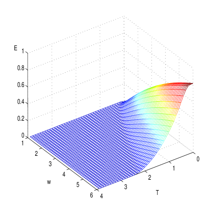
Figure 1: Entanglement of the two oscillators as a function of the natural frequency and temperature. The threshold temperature increases almost linearly with frequency.

The maximum entanglement behaves like $\ \ (\frac{1}{16\ln 2}+\frac{1}{4}-\frac{1}{8}\log_{2}(w-1))(w-1)^{2}\$ for small frequencies $\ \omega\approx 1(\omega_{0}<<1)\$ and like $\ \ \frac{1}{\ln 2}-2+\frac{1}{2}\log_{2}\omega\$ for large frequencies $\ \omega>>1$.

In summary we have set up an easy formalism for calculating the thermal entanglement of arbitrary bosonic modes in a rather large class of problems. For example the formalism can be applied to arbitrary lattices of bosonic modes to see how thermal fluctuations affect frustration of entanglement [21], or to a chain of coupled oscillators. In the later case the entanglement can be obtained as a function of both the temperature and the distance between the particles. This is in contrast to the spin systems where due to the complicated nature of their spectrum this later dependence can not be obtained except only at low temperatures and under certain assumptions [22].
I would like to thank V. Karimipour, A. Bayat, I. Marvian, L. Memarzadeh and A. Sheikhan for very valuable discussions.

References

[1] T. Osborne, M. Nielsen,Physical Review A 66 (03) 032110 (2002).
[2] M. C. Arnesen, S. Bose, and V. Vedral, Phys. Rev. Lett. 87, 277901 (2001).
[3] M. K. O’Connor and W. K. Wootters, Phys. Rev. A 63, 052302 (2001).
[4] W. K. Wootters, Phys.Rev.Lett. 80, 2245 (1998).
[5] M. A. Nielsen and I. L. Chuang, Quantum Computation and Quantum
Information, Cambrdige 2000.
[6] A. Osterloh, L. Amico, G. Falci, and R. Fazio, Nature 416, 608 (2002).
[7]G. Giedke, M. M. Wolf, O. Kruger, R. F. Werner, and
J. I. Cirac, Phys Rev Lett. 91,107901(2003).
[8]S. L. Braunstein and A. K. Pati, eds., Quantum Information with Continuous
Variables (Kluwer Academic, Dordrecht, 2003).
[9] S. J. van Enk, Phys. Rev. A 67, 022303 (2003).
[10]J. R. Gittings and A. J. Fisher, Phys. Rev. A 66, 032305 (2002).
[11] Y. Shi, Phys. Rev. A 67, 024301 (2003).
[12] P. Zanardi, Phys. Rev. A 65, 042101 (2002).
[13] V. Vedral, Central Eur. J. Phys. 1, 289
(2003).
[14] F. Grosshans, et al., Nature (London) 421,
238 (2003).
[15] B. Englert and K. Wodkiewicz, Int. J. Quant. Inf., vol 1, No. 2, (2003) 153-188.
[16]G. Giedke, B. Kraus, M. Lewenstein and J. I.
Cirac, Phys. Rev. Lett. 87, 167904 (2001).
[17]M. C. de Oliveira, Phys. Rev. A 70, 034303 (2004).
[18] G. Giedke, L. M. Duan, I. Cirac and P. Zoller,
Int. J. Quant. Inf., vol I, No. 3 (2001) 79-86.
[19] A. Serafini, F. Illuminati, and S. De Siena, J. Phys. B 37, L21
(2004).
[20]X. Wang, and P. Zanardi, Phys. Lett. A 301 (1-2), 1 (2002).
[21]M. M. Wolf, F. Verstraete, and J. I. Cirac,Phys. Rev. Lett. 92, 087903 (2004)
[22] M. Asoudeh, and V. Karimipour, Phys. Rev. A 70, 052307 (2004).