Continuous-Variable Spatial Entanglement for Bright Optical Beams

Abstract

A light beam is said to be position squeezed if its position can be determined to an accuracy beyond the standard quantum limit. We identify the position and momentum observables for bright optical beams and show that position and momentum entanglement can be generated by interfering two position, or momentum, squeezed beams on a beam splitter. The position and momentum measurements of these beams can be performed using a homodyne detector with local oscillator of an appropriate transverse beam profile. We compare this form of spatial entanglement with split detection-based spatial entanglement.

I Introduction

The concept of entanglement was first proposed by Einstein, Podolsky and Rosen in a seminal paper in 1935 EPR . The original Einstein-Podolsky-Rosen (EPR) entanglement, as discussed in the paper, involved the position and momentum of a pair of particles. In this article, we draw an analogy between the original EPR entanglement and the position and momentum ($x$-$p$) entanglement of bright optical beams.

Entanglement has been reported in various manifestations. For continuous wave (CW) optical beams, these include, quadrature silberhorn ; ou and polarisation bowen-pol entanglement. Spatial forms of entanglement, although well studied in the single photon regime, have not been studied significantly in the continuous wave regime. Such forms of entanglement are interesting as they span a potentially infinite Hilbert space. Spatial EPR entanglement lugiato has wide-ranging applications from two-photon quantum imaging abouraddy ; pittman to holographic teleportation abouraddy1 ; sokolov and interferometric faint phase object quantum imaging sokolov1 .

Current studies are focused on $x$-$p$ entanglement for the few photons regime. Howell et al. howell observed near and far-field quantum correlation, corresponding to the position and momentum observables of photon pairs. Gatti et al. gatti4 have also discussed the spatial EPR aspects in the photons pairs emitted from an optical parametric oscillator below threshold. Other forms of spatial entanglement which are related to image correlation have also been investigated. A scheme to produce spatially entangled images between the signal and idler fields from an optical parametric amplifier has been proposed by Gatti et al. gatti ; gatti1 . Their work was extended to the macroscopic domain by observing the spatial correlation between the detected signal and idler intensities, generated via the parametric down conversion process gatti3 .

Our proposal considers the possibility of entangling the position and momentum of a free propagating beam of light, as opposed to the entanglement of local areas of images, considered in previous proposals. Our scheme is based on the concept of position squeezed beams where we have shown that we have to squeeze the transverse mode corresponding to the first order derivative of the mean field in order to generate the position squeezed beam hsu . Similarly to the generation of quadrature entangled beams, the position squeezed beams are combined on a beam-splitter to generate $x$-$p$ entangled beams. We also propose to generate spatial entanglement for split detection, utilising spatial squeezed beams reported by Treps et al. treps1d ; treps2d ; treps2dlong . This form of spatial entanglement has applications in quantum imaging systems.

We first define the position and momentum of an optical beam by performing a multi-modal decomposition on a displaced and tilted beam, respectively. We consider the case of a TEM₀₀ beam and show that the corresponding position and momentum observables are conjugate observables which obey the Heisenberg commutation relation. We then propose a scheme to produce $x$-$p$ entanglement for TEM₀₀ optical beams. Finally, we consider spatial squeezed beams for split detectors and show that it is also possible to generate spatial entanglement with such beams.

II Position-Momentum Entanglement

II.1 Definitions - Classical Treatment

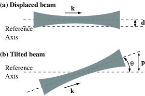
Figure 1: (a) Beam displacement $d$, and (b) beam tilt by angle $\theta$, from a reference axis.

Let us consider an optical beam with $x$- and $y$- symmetric transverse intensity profile propagating along the $z$-axis. Since the axes of symmetries remain well defined during propagation, we can relate the beam position relative to these axes. To simplify our analysis we henceforth assume without loss of generality, a one-dimensional beam displacement, $d$, from the reference $x$-axis (see Fig. 1(a)). We denote the electric field profile of the beam by $E(x)$. For a displaced beam, the electric field profile is given by

$$E_{d}(x)=E(x)+d\frac{\partial E(x)}{\partial x}+\frac{d^{2}}{2}\frac{\partial^{2}E(x)}{\partial x^{2}}+\cdots$$ (1)

In the regime where displacement is much smaller than the beam size, we can utilise the linearised approximation where only the zeroth and first order terms are significant. We see from this expression that the zeroth order term is not dependent on $d$, and that the displacement is directly proportional to the derivative of the field amplitude $\partial E(x)/\partial x$ hsu .

The transverse beam momentum $p$ on the other hand, can be obtained from the transverse component of the wave-number of the beam, $p=k\sin\theta$, where $k=2\pi/\lambda$ and the beam tilt is $\theta$. This beam tilt is defined with respect to a pivot point at the beam waist, as shown in Fig. 1(b).

The electric field profile for a tilted beam with untilted electric field profile $E(x)$ and wavelength $\lambda$ is given by

$$E_{\theta}(x)=\exp\left[\frac{i2\pi x\sin\theta}{\lambda}\right]E(x\cos\theta)$$ (2)

We can again simplify Eq. (2) by taking the zeroth and first order Taylor expansion terms to get a transverse beam momentum of $p\simeq k\theta$. In the case of small displacement or tilt, we therefore obtain a pair of equations

$$E_{d}(x) \approx E(x)+\ d \!\frac{\partial E(x)}{\partial x}$$ (3)

$$E_{p}(x) \approx E(x)+\ p \!ixE(x)$$ (4)

Eqs. (3) and (4) give the field parameters that relate to the displacement and tilt of a beam. For freely propagating optical modes, the Fourier transform of the derivative of the electric field, ${\cal F}(\partial E(x)/\partial x)$, is of the form $ix{E}(x)$. Hence, the Fourier transform of displacement is tilt.

In the case of a single photon, the position and momentum are defined by considering the spatial probability density of the photon, given by $|E(x)|^{2}/I$, where $I=\int|E(x)|^{2}dx$ is the normalisation factor. The mean position obtained from an ensemble of measurements on single photons is then given by $\langle x\rangle=\frac{1}{I}\int x|E(x)|^{2}dx$. The momentum of the photon is defined by the spatial probability density of the photon in the far-field, or equivalently by taking the Fourier transform of $\langle x\rangle$. These definitions are consistent with our definitions of position and momentum for bright optical modes.

II.2 TEM_pq Basis

In theory, spatial entanglement can be generated for fields with any arbitrary transverse mode-shape. However, as with other forms of continuous-variable entanglement, the efficacy of protocols to generate entanglement is highest if the initial states are minimum uncertainty. For position and momentum variables, the minimum uncertainty states are those which satisfy the Heisenberg uncertainty relation $\Delta^{2}\hat{x}\Delta^{2}\hat{p}\geq\hbar$, in the equality. This equality is only satisfied by states with Gaussian transverse distributions griffiths , therefore we limit our analysis to that of TEM₀₀ modes.

A field of frequency $\omega$ can be represented by the positive frequency part of the mean electric field $\mathcal{E}^{+}e^{i\omega t}$. We are interested in the transverse information of the beam described fully by the slowly varying field envelope $\mathcal{E}^{+}$. We express this field in terms of the TEM_pq modes. For a measurement performed in an exposure time $T$, the mean field for a displaced TEM₀₀ beam can be written as

$$\mathcal{E}_{d}^{+}(x)=i\sqrt{\frac{\hbar\omega}{2\epsilon_{0}cT}}\sqrt{N}\Big{(}u_{0}(x)+\frac{d}{w_{0}}u_{1}(x)\Big{)}$$ (5)

where the first term indicates that the power of the displaced beam is in the TEM₀₀ mode while the second term gives the displacement signal contained in the amplitude of the TEM₁₀ mode component. The corresponding mean field for a tilted TEM₀₀ beam can be written as

$$\mathcal{E}_{p}^{+}(x)=i\sqrt{\frac{\hbar\omega}{2\epsilon_{0}cT}}\sqrt{N}\Big{(}u_{0}(x)+\frac{iw_{0}p}{2}u_{1}(x)\Big{)}$$ (6)

where the second term describes the beam momentum signal, contained in the $\pi/2$ phase-shifted TEM₁₀ mode component.

II.3 Definitions - Quantum Treatment

We now introduce a quantum mechanical representation of the beam by taking into account the quantum noise of optical modes. We can write the positive frequency part of the electric field operator in terms of photon annihilation operators $\hat{a}$. The field operator is given by

$$\hat{\mathcal{E}}_{\rm in}^{+}=i\sqrt{\frac{\hbar\omega}{2\epsilon_{0}cT}}\sum_{n=0}^{\infty}\hat{a}_{n}u_{n}(x)$$ (7)

where $u_{n}(x)$ are the transverse beam amplitude functions for the TEM_pq modes and $\hat{a}_{n}$ are the corresponding annihilation operators. $\hat{a}_{n}$ is normally written in the form of $\hat{a}_{n}=\langle\hat{a}_{n}\rangle+\delta\hat{a}_{n}$, where $\langle\hat{a}_{n}\rangle$ describes the coherent amplitude part and $\delta\hat{a}_{n}$ is the quantum noise operator.

In the small displacement and tilt regime, the TEM₀₀ and TEM₁₀ modes are the most significant hsu , with the TEM₁₀ mode contributing to the displacement and tilt signals. We can rewrite the electric field operator for mean number of photons $N$ as

$$\hat{\mathcal{E}}_{in}^{+} = i\sqrt{\frac{\hbar\omega}{2\epsilon_{0}cT}}\Big{(}\sqrt{N}u_{0}(x)+\frac{\delta\hat{X}_{a_{0}}^{+}+i\delta\hat{X}_{a_{0}}^{-}}{2}$$ (8)

$$+\sum_{n=1}^{\infty}\Big{(}\frac{\hat{X}_{a_{i}}^{+}+i\hat{X}_{a_{i}}^{-}}{2}\Big{)}u_{i}(x)\Big{)}$$

where the annihilation operator is now written in terms of the amplitude $\hat{X}_{a}^{+}$ and phase $\hat{X}_{a}^{-}$ quadrature operators.

The displacement and tilt of a TEM₀₀ beam is given by the amplitude and phase of the $u_{1}(x)$ mode in Eqs. (5) and (6), respectively. We can, therefore, write the beam position and momentum operators as

$$\hat{x} = \frac{w_{0}}{2\sqrt{N}}\hat{X}_{a_{1}}^{+}$$ (9)

$$\hat{p} = \frac{1}{w_{0}\sqrt{N}}\hat{X}_{a_{1}}^{-}$$ (10)

II.4 Commutation Relation

Two observables corresponding to the position and momentum of a TEM₀₀ beam have been defined. We have shown that the position and momentum observables correspond to near- and far-field measurements of the beam, respectively. Hence, we expect from Eqs. (9) and (10), that the position and momentum observables do not commute. Indeed, the commutation relation between the two quadratures of the TEM₁₀ mode is $[\hat{X}_{a_{1}}^{+},\hat{X}_{a_{1}}^{-}]=2i$. This leads to the commutation relation between the position and momentum observables of an optical beam with $N$ photons

$$[\hat{x},\hat{p}]=\frac{i}{N}$$ (11)

This commutation relation is similar to the position-momentum commutation relation for a single photon, aside from the $1/N$ factor. The $1/N$ factor is related to the precision with which one can measure beam position and momentum. Rewriting the Heisenberg inequality using the commutation relation, gives

$$\Delta^{2}\hat{x}\Delta^{2}\hat{p}\geq\frac{1}{4N}.$$ (12)

The position measurement of a coherent optical beam gives a signal which scales with $N$. The associated quantum noise of the position measurement scales with $\sqrt{N}$. Hence the positioning sensitivity of a coherent beam scales as $\sqrt{N}$ hsu ; treps1d . The same consideration applied to the sensitivity of beam momentum measurement shows an equivalent dependence of $\sqrt{N}$. This validates the factor of $N$ in the Heisenberg inequality and the commutation relation for a CW optical beam.

II.5 Entanglement Scheme

We have shown that the position and momentum observables of CW TEM₀₀ optical beams satisfy the Heisenberg commutation relation. Consequently, EPR entanglement for the position and momentum of TEM₀₀ beams is possible. Experimentally, the usual quadrature entanglement is generated by mixing two amplitude squeezed beams on a 50:50 beamsplitter. The same idea can be applied to generate EPR $x$-$p$ entanglement, by using position squeezed beams hsu . Our scheme to produce $x$-$p$ entanglement between two CW TEM₀₀ optical beams is shown in Figure 2.

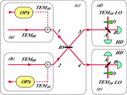
Figure 2: Scheme for generating position-momentum entanglement for continuous wave TEM₀₀ optical beams. OPA: optical parametric amplifiers for the generation of squeezed light, BS: 50:50 beam-splitter, HD: homodyne detectors, LO: local oscillator beams, $\phi$: phase of local oscillator beam.

The position squeezed beams in (a) and (b) are generated via the in-phase combination of a vacuum squeezed TEM₁₀ beam with a coherent TEM₀₀ beam. Such beam combination can be achieved experimentally, for example using an optical cavity or a beam-splitter treps2dlong . The result of the combination is a position squeezed beam. To generate entanglement, we consider beams with zero mean position and momentum, but we are interested in the quantum noise of the position and momentum of the beam. With this assumption, the electric field operators for the two input beams at the beam-splitter are given by

$$\hat{\mathcal{E}}_{1}^{+}=i\sqrt{\frac{\hbar\omega}{2\epsilon_{0}cT}}\Big{(}\sqrt{N}u_{0}(x)+\sum_{n=0}^{\infty}\delta\hat{a}_{n}u_{n}(x)\Big{)}$$ (13)

$$\hat{\mathcal{E}}_{2}^{+}=i\sqrt{\frac{\hbar\omega}{2\epsilon_{0}cT}}\Big{(}\sqrt{N}u_{0}(x)+\sum_{n=0}^{\infty}\delta\hat{b}_{n}u_{n}(x)\Big{)}$$ (14)

where in both equations, the first bracketed term describes the coherent amplitude of the TEM₀₀ beam. The second bracketed terms describe the quantum fluctuations present in all modes. For position squeezed states, only the TEM₁₀ mode is occupied by a vacuum squeezed mode. All other modes are occupied by vacuum fluctuations. It is also assumed that the number of photons in each of the two beams, during the measurement window, is equal to $N$. The two position squeezed beams (1,2) are combined in-phase on a 50:50 beam-splitter (BS) in (c).

The usual input-output relations of a beam-splitter apply. The electric field operators describing the two output fields from the beam-splitter are given by $\hat{\mathcal{E}}_{3}=(\hat{\mathcal{E}}_{1}+\hat{\mathcal{E}}_{2})/\sqrt{2}$ and $\hat{\mathcal{E}}_{4}=(\hat{\mathcal{E}}_{1}-\hat{\mathcal{E}}_{2})/\sqrt{2}$. To demonstrate the existence of entanglement, we seek for quantum correlation and anti-correlation between the position and momentum quantum noise operators. The position operator corresponding to beams 3 and 4 are given respectively by

$$\delta\hat{x}_{3} = \frac{w_{0}}{2\sqrt{2}\sqrt{N}}\Big{(}\delta\hat{X}_{a_{1}}^{+}+\delta\hat{X}_{b_{1}}^{-}\Big{)}$$ (15)

$$= \frac{1}{\sqrt{2}}\Big{(}\delta\hat{x}_{a}+\frac{w_{0}^{2}}{2}\delta\hat{p}_{b}\Big{)}$$

$$\delta\hat{x}_{4} = \frac{w_{0}}{2\sqrt{2}\sqrt{N}}\Big{(}\delta\hat{X}_{a_{1}}^{+}-\delta\hat{X}_{b_{1}}^{-}\Big{)}$$ (16)

$$= \frac{1}{\sqrt{2}}\Big{(}\delta\hat{x}_{a}-\frac{w_{0}^{2}}{2}\delta\hat{p}_{b}\Big{)}$$

The momentum operator corresponding to the photo-current difference for beams 3 and 4 are given by

$$\delta\hat{p}_{3} = \frac{1}{w_{0}\sqrt{2\sqrt{N}}}\Big{(}\delta\hat{X}_{a_{1}}^{-}+\delta\hat{X}_{b_{1}}^{+}\Big{)}$$ (17)

$$= \frac{1}{\sqrt{2}}\Big{(}\delta\hat{p}_{a}+\frac{2}{w_{0}^{2}}\delta\hat{x}_{b}\Big{)}$$

$$\delta\hat{p}_{4} = \frac{1}{w_{0}\sqrt{2\sqrt{N}}}\Big{(}\delta\hat{X}_{a_{1}}^{-}-\delta\hat{X}_{b_{1}}^{+}\Big{)}$$ (18)

$$= \frac{1}{\sqrt{2}}\Big{(}\delta\hat{p}_{a}-\frac{2}{w_{0}^{2}}\delta\hat{x}_{b}\Big{)}$$

In our case where the two input beams are position squeezed, the sign difference between the position noise operators in Eqs. (15) and (16) as well as that between the momentum noise operators in Eqs. (17) and (18) are signatures of correlation and anti-correlation for $\delta\hat{x}$ and $\delta\hat{p}$.

II.6 Inseparability Criterion

Many criterions exist to characterise entanglement, for example the inseparability criterion duan and the EPR criterion reid . We have adopted the inseparability criterion to characterise position-momentum entanglement. For states with Gaussian noise statistics, Duan et al. duan have shown that the inseparability criterion is a necessary and sufficient criterion for EPR entanglement.

In the case where two beams are perfectly interchangeable and have symmetrical fluctuations in the amplitude and phase quadratures, the inseparability criterion has been generalised and normalised to a product form given by bowen-pol ; bowen-pol1 ; bowen-epr ; bowen-epr1 ; tan ; mancini

$$\mathcal{I}(\hat{x},\hat{p})=\frac{\langle(\hat{x}_{3}+\hat{x}_{4})^{2}\rangle\langle(\hat{p}_{3}-\hat{p}_{4})^{2}\rangle}{|[\hat{x},\hat{p}]|^{2}}$$ (19)

for any pair of conjugate observables $\hat{x}$ and $\hat{p}$, and a pair of beams denoted by the subscripts 3 and 4. For states which are inseparable, $\mathcal{I}(\delta\hat{x},\delta\hat{p})<1$. By using observables $\delta\hat{x}$ and $\delta\hat{p}$ from Eqs. (15), (16), (17) and (18) as well as the commutation relation of Eq. (11) the inseparability criterion for beams 3 and 4 is given by

$$\mathcal{I}(\delta\hat{x},\delta\hat{p}) = \frac{16N^{2}}{\omega_{0}^{4}}\langle(\delta\hat{x}_{a_{1}}^{+})^{2}\rangle\langle(\delta\hat{x}_{b_{1}}^{+})^{2}\rangle$$ (20)

$$= \langle(\delta\hat{X}_{a_{1}}^{+})^{2}\rangle\langle(\delta\hat{X}_{b_{1}}^{+})^{2}\rangle$$

$$< 1$$

where we have assumed that the TEM₁₀ modes of beams 1 and 2 are amplitude squeezed (i.e. $\langle(\delta\hat{X}_{a_{1}}^{+})^{2}\rangle<1$ and $\langle(\delta\hat{X}_{b_{1}}^{+})^{2}\rangle<1$).

Thus we have demonstrated that CV EPR entanglement between the position and momentum observables of two CW beams can be achieved.

II.7 Detection Scheme

Ref. hsu has shown that the optimum small displacement measurement is homodyne detection with a TEM₁₀ local oscillator beam (see Fig. 2 (d)). When the input beam is centred with respect to the TEM₁₀ local oscillator beam, no power is contained in the TEM₁₀ mode. Due to the orthogonality of Hermite-Gauss modes, the TEM₁₀ local oscillator only detects the TEM₁₀ vacuum noise component. As the input beam is displaced, power is coupled into the TEM₁₀ mode. This coupled power interferes with the TEM₁₀ local oscillator beam, causing a change in photo-current observed at the output of the homodyne detector. Thus the difference photo-current of the TEM₁₀ homodyne detector is given by hsu

$$\hat{n}_{-}^{d}=\frac{2\sqrt{N}\sqrt{N_{\rm LO}}}{w_{0}}\hat{x}$$ (21)

where $N_{\rm LO}$ and $N$ are the total number of photons in the local oscillator and displaced beams, respectively, with $N_{\rm LO}\gg N$. The linearised approximation is utilised, where second order terms in $\delta\hat{a}$ are neglected since $N\gg|\langle\delta\hat{a}_{n}^{2}\rangle|$ for all $n$.

In order to measure momentum, one could use a lens to Fourier transform to the far-field plane, where the beam is then measured using the TEM₁₀ homodyning scheme. However, we have shown that the the position and momentum of a TEM₀₀ beam differs by the phase of the TEM₁₀ mode component. Indeed for a tilted TEM₀₀ beam, the TEM₁₀ mode component is $\pi/2$ phase shifted relative to the TEM₀₀ mode component. Consequently the phase quadrature of the TEM₁₀ mode has to be interrogated. This can be achieved by utilising a TEM₁₀ local oscillator beam with a $\pi/2$ phase difference relative to the TEM₁₀ mode component of the TEM₀₀ beam. The resulting photo-current difference between the two homodyning detectors, for $N_{\rm LO}\gg N$, is given by

$$\hat{n}_{-}^{p}=w_{0}\sqrt{N}\sqrt{N_{\rm LO}}\hat{p}$$ (22)

III Spatial entanglement for split detection

The entanglement presented in the previous section is analogous to $x$-$p$ entanglement in the single photon regime. However, the choice of the mean field mode is restricted to the TEM₀₀ mode. This limits the richness of a spatial variable and thus excludes the possibility of generating an infinite Hilbert space. To exploit the properties of spatial variables, we now consider more traditional forms of spatial squeezing. Consequently, we study the possibility of generating spatial entanglement for array detection devices, based on spatial squeezed beams.

III.1 Spatial Squeezing

Spatial squeezing was first introduced by Kolobov Kolobov . The generation of spatial squeezed beams for split and array detectors was experimentally demonstrated by Treps et al. treps2d ; treps2dlong ; treps1d . A one-dimensional spatial squeezed beam has a spatially ordered distribution, where there exists correlation between the photon numbers in both transverse halves of the beam. A displacement signal applied to this beam can thus be measured to beyond the QNL.

We consider a beam of normalised transverse amplitude function $v_{0}(x)$ incident on a split detector. The noise of split detection has been shown to be due to the flipped mode fabre , given by

$$v_{1}(x)=\left\{\begin{array}[]{ll}v_{0}(x)&\textrm{for }x>0\\ -v_{0}(x)&\textrm{for }x<0\end{array}\right.$$

When the field is centred at the split-detector, such that the mean value of the measurement is zero, the flipped mode is thus orthogonal to the mean field mode. In this instance, modes $v_{i}(x)$ (for $i>1$) can be derived to complete the modal basis. The electric field operator written in this new modal basis is given by

$$\hat{\mathcal{E}}^{+}=i\sqrt{\frac{\hbar\omega}{2\epsilon_{0}cT}}\Big{(}\sqrt{N}v_{0}(x)+\sum_{n=0}^{\infty}\delta\hat{c}_{n}v_{n}(x)\Big{)}$$ (23)

where the first term describes the coherent excitation of the beam in the $v_{0}(x)$ mode and $N$ is the total number of photons in the beam. It has been shown that the corresponding photon number difference operator for split detection is given by hsu

$$\hat{n}_{-}^{(+)}=\sqrt{N}\delta\hat{X}_{c_{0}}^{+}$$ (24)

The beam is spatially squeezed if the state of the flipped mode is vacuum squeezed and in phase with the mean field mode (see Fig. 3 (a) and (b)).

III.2 Spatial Homodyne

Since split detection is commonly used as a detection device for beam position, one would naturally consider taking the Fourier transform of a spatial squeezed beam to obtain the conjugate observable for the beam. However, we have shown that split detection does not correspond exactly to beam position measurement. Thus the Fourier plane of the spatial squeezed beam does not provide the conjugate observable. More practically, the flipped mode is not mode-shape invariant under Fourier transformation. In the far-field, each odd-ordered mode component of the flipped mode obtains a $(2n+1)\pi$ Gouy phase difference, compared to the near-field. Thus the mode-shape in the far-field is no longer a flipped mode. Consequently, far and near-field measurements of a spatial squeezed beam will not give the conjugate observables.

However, we can find the conjugate observables of a spatial squeezed beam by drawing an analogy to standard homodyne detection. In split detection, the equivalent local oscillator mode is the mean field $v_{0}(x)$ mode. The mode under interrogation by the split detector is the flipped mode $v_{1}(x)$. In the case of homodyne detection, the phase of the local oscillator beam is varied to measure the conjugate observables (i.e. amplitude and phase quadratures) of the input beam. Adapting this concept to the split detector, the conjugate observables for the spatial squeezed beam is thus the amplitude and phase quadratures of the flipped mode, while the mode-shape of the flipped mode remains unaltered. This is further verified upon inspection of Eq. (24).

Our scheme to perform a phase measurement of the flipped mode is shown in Fig. 3 (d). In our scheme we assume that the mean field is a TEM₀₀ mode. Note that in principle, this analysis could be performed for any mode-shape. The coherent TEM₀₀ mode component provides a phase reference for the flipped mode, analogous to that of a local oscillator beam in homodyne detection. Thus the phase quadrature of the flipped mode can be accessed by applying a $\pi/2$ phase shift between the the TEM₀₀ mode and the flipped mode noise component. Experimentally, this is achievable using an optical cavity. When the cavity is non-resonant for the $v_{0}(x)$ and $v_{1}(x)$ modes it will reflect off the two modes, in phase, onto the split detector. This will give a measurement of the amplitude quadrature of the flipped mode. However, the cavity can be tuned to be partially resonant on the $v_{0}(x)$ mode while reflecting the flipped mode. A $\pi/2$ phase difference can then be introduced between the reflected $v_{0}(x)$ and $v_{1}(x)$ modes, giving a measurement of the phase quadrature of the flipped mode. The corresponding photon number difference operator is

$$\hat{n}_{-}^{(-)}=\sqrt{N}\delta\hat{X}_{c_{0}}^{-}$$ (25)

which is the orthogonal quadrature of the spatial squeezed beam. The photon number operators corresponding to the two measurements in Eqs. (24) and (25) are conjugate observables and satisfy the commutation relation $[\hat{n}_{-}^{(+)},\hat{n}_{-}^{(-)}]=2iN$.

It is important to realise that the number of photons $N$ in Eqs. (24) and (25) are only approximately equal. This is due to the fact that partial power in the TEM₀₀ mode is transmitted by the cavity, when the cavity is partially resonant on the TEM₀₀ mode. Although it is possible to implement a scheme that conserves the total number of photons at detection (e.g. losslessly separating the mean field and flipped modes and recombining them with a phase difference), we would like to emphasise that our scheme is more simple and intuitive, as well as being valid when $N$ is large.

III.3 Entanglement Scheme

In order to generate spatial entanglement for split detection, two spatial squeezed beams labelled 1 and 2 are combined on a 50:50 beam-splitter, as shown in Figure 3 (c).

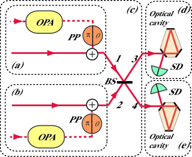
Figure 3: Scheme for generating spatial entanglement for TEM₀₀ continuous wave light beams. OPA: optical parametric amplifiers for generating squeezed beams, PP: phase plates for producing flipped modes, BS: 50:50 beam-splitter.

The electric field operators for the two input spatial squeezed beams at the beam-splitter are described in a form identical to that of Eq. (23). The annihilation operators of the electric field operators for input beams 1 and 2 are labelled by $\hat{c}_{n}$ and $\hat{d}_{n}$, respectively. By following a similar procedure as before, the photon number difference operator for output beams 3 and 4 from the beam-splitter are calculated.

For the amplitude quadrature measurement, the addition of the difference photo-current between beams 3 and 4 yields

$$\hat{n}_{3-}^{(+)}+\hat{n}_{4-}^{(+)}=\sqrt{N}(\delta\hat{X}_{c_{0}}^{+}+\delta\hat{X}_{d_{0}}^{+})$$ (26)

For the phase quadrature measurement, the subtraction of the difference photo-current between beams 3 and 4 gives

$$\hat{n}_{3-}^{(-)}-\hat{n}_{4-}^{(-)}=\sqrt{N}(\delta\hat{X}_{d_{0}}^{+}-\delta\hat{X}_{c_{0}}^{+})$$ (27)

To verify spatial entanglement, the inseparability criterion is utilised. The substitution of Eqs. (26), (27) and the commutation relation between the photon number difference operators into the generalised form of the inseparability criterion gives

$$\mathcal{I}(\delta\hat{n}_{-}^{(+)},\delta\hat{n}_{-}^{(-)}) = \frac{N\left(V_{c_{0}}^{2}+2V_{c_{0}}V_{d_{0}}+V_{d_{0}}^{2}\right)}{4N}$$ (28)

$$< 1$$

where $V_{c_{0}}=\langle(\delta\hat{X}_{c_{0}}^{+})^{2}\rangle$ and $V_{d_{0}}=\langle(\delta\hat{X}_{d_{0}}^{+})^{2}\rangle$ are the variances for the flipped mode component of the spatial squeezed beams 1 and 2. The inseparability criterion is satisfied for amplitude squeezed flipped modes $V_{c_{0}}<1$ and $V_{d_{0}}<1$.

We have proposed a scheme to generate spatial entanglement for split detection, using spatial squeezed beams. Spatial squeezing has been defined for any linear measurement performed with an array detector trepsmulti . Similarly, spatial entanglement corresponding to any linear measurement, can be obtained. For an infinite span array detector with infinitessimally small pixels, it is thus possible to generate multi-mode spatial entanglement, increasing the Hilbert space to being infinite-dimensional.

IV Conclusion

We have identified the position and momentum of a TEM₀₀ optical beam. By showing that $\hat{x}$ and $\hat{p}$ are conjugate observables that satisfy the Heisenberg commutation relation, a continuous variable $x$-$p$ entanglement scheme is proposed. This proposed entanglement, as considered by EPR EPR , was characterised using a generalised form of the inseparability criterion.

We further explored a form of spatial entanglement which has applications in quantum imaging. The detection schemes for quantum imaging are typically array detectors. In this article, we considered the split detector. We utilised the one-dimensional spatial squeezing work of Treps et al. treps1d and proposed a spatial homodyning scheme for the spatial squeezed beam. By identifying the conjugate observables for the spatial squeezed beam as the amplitude and phase quadratures of the flipped mode, we showed that split detection-based spatial entanglement can be obtained.

- (1) A. Einstein, B. Podolsky and N. Rosen, Phys. Rev. 47, 777 (1935)
- (2) Ch. Silberhorn, P. K. Lam, O. Weiss, F. König, N. Korolkova and G. Leuchs, Phys. Rev. Lett. 86, 4267 (2001).
- (3) Z. Y. Ou, S. F. Pereira, H. J. Kimble and K .C. Peng, Phys. Rev. Lett. 68, 3664 (1992).
- (4) W. P. Bowen, N. Treps, R. Schnabel and P. K. Lam, Phys. Rev. Lett. 89, 253601 (2002).
- (5) J. C. Howell, R. S. Bennick, S. J. Bentley and R. W. Boyd, Phys. Rev. Lett. 92, 210403 (2003).
- (6) A. Gatti and L. A. Lugiato, Phys. Rev. A 52, 1675 (1995).
- (7) A. Gatti, E. Brambilla, L. A. Lugiato and M. I. Kolobov, Phys. Rev. Lett. 83, 1763 (1999).
- (8) A. Gatti, E. Brambilla, L. A. Lugiato and M. I. Kolobov, J. Opt. B 2, 196 (2000).
- (9) A. Gatti, L. A. Lugiato, K. I. Petsas and I. Marzoli, Europhys. Lett. 46, 461 (1999).
- (10) A. Gatti, E. Brambilla and L. A. Lugiato, Phys. Rev. Lett. 90, 133603 (2003).
- (11) L. A. Lugiato, A. Gatti and E. Brambilla, J. Opt. B 4, S176 (2002).
- (12) A. F. Abouraddy, B. E. A. Saleh, A. V. Sergienko and M. C. Teich, Phys. Rev. Lett. 87, 123602 (2001).
- (13) T. B. Pittman, Y. H. Shih, D. V. Strekalov and A. V. Sergienko, Phys. Rev. A 52, R3429 (1995).
- (14) A. F. Abouraddy, B. E. A. Saleh, A. V. Sergienko and M. C. Teich, Opt. Exp. 9, 498 (2001).
- (15) I .V. Sokolov, M. I. Kolobov, A. Gatti and L. A. Lugiato, Opt. Comm. 193, 175 (2001).
- (16) I. V. Sokolov, J. Opt. B 2, 179 (2000).
- (17) M. T. L. Hsu, V. Delaubert, P. K. Lam and W. P. Bowen, J. Opt. B 6, 495 (2004).
- (18) D. J. Griffiths, Introduction to Quantum Mechanics, Prentice-Hall Inc., New Jersey (1995).
- (19) N. Treps, U. Andersen, B. Buchler, P. K. Lam, A. Maître, H.-A. Bachor and C. Fabre, Phys. Rev. Lett. 88, 203601 (2002).
- (20) N. Treps, N. Grosse, W. P. Bowen, C. Fabre, H.-A. Bachor and P. K. Lam, Science 301, 940 (2003).
- (21) N. Treps, N. Grosse, W. P. Bowen, M. T. L. Hsu, A. Maître, C. Fabre, H.-A. Bachor and P. K. Lam, J. Opt. B 6, S664 (2004).
- (22) L.-M. Duan, G. Giedke, J. I. Cirac and P. Zoller, Phys. Rev. Lett. 84, 2722 (2000)
- (23) M. D. Reid and P. D. Drummond, Phys. Rev. Lett. 60, 2731 (1988)
- (24) C. Fabre, J. B. Fouet and A. Maître, Opt. Lett., 76, 76 (2000).
- (25) M. I. Kolobov, Rev. Mod. Phys, 71, 1539 (1999)
- (26) N. Treps, V. Delaubert, A. Maître, J. M. Courty and C. Fabre, quant-ph/0407246.
- (27) W. P. Bowen, N. Treps, R. Schnabel and P. K. Lam, Phys. Rev. Lett. 89, 253601 (2002).
- (28) W. P. Bowen, R. Schnabel, P. K. Lam and T. C. Ralph, Phys. Rev. Lett. 90, 043601 (2003).
- (29) W. P. Bowen, R. Schnabel, P. K. Lam and T. C. Ralph, Phys. Rev. A 69, 012304 (2004).
- (30) S. Tan, Phys. Rev. A 60, 2752 (1999).
- (31) S. Mancini, V. Giovannetti, D. Vitali and P. Tombesi, Phys. Rev. Lett. 88, 120401 (2002).