Radiative Corrections to Multi–Level Mollow–Type Spectra

Abstract

This paper is concerned with two rather basic phenomena: the incoherent fluorescence spectrum of an atom driven by an intense laser field and the coupling of the atom to the (empty) modes of the radiation field. The sum of the many-photon processes gives rise to the inelastic part of the atomic fluorescence, which, for a two-level system, has a well-known characteristic three-peak structure known as the Mollow spectrum. From a theoretical point of view, the Mollow spectrum finds a natural interpretation in terms of transitions among laser-dressed states which are the energy eigenstates of a second-quantized two-level system strongly coupled to a driving laser field. As recently shown, the quasi-energies of the laser-dressed states receive radiative corrections which are nontrivially different from the results which one would expect from an investigation of the coupling of the bare states to the vacuum modes. In this article, we briefly review the basic elements required for the analysis of the dynamic radiative corrections, and we generalize the treatment of the radiative corrections to the incoherent part of the steady-state fluorescence to a three-level system consisting of $1S$, $3P$ and $2S$ states.

I Introduction

The theory of the interactions of atoms with light began in the 1920s and 1930s with the description of a number of basic processes; one of these is the Kramers–Heisenberg formula Kramers and Heisenberg (1925) which describes a process in which an electron absorbs and emits one photon. The corresponding Feynman diagram is shown in Fig. 1 (a). This scattering process is elastic, the electron radiates at exactly the driving frequency, a point which has been stressed a long time ago Weisskopf (1931). If more than one photon is absorbed or emitted, then the energy conservation applied only to the sum of the frequencies of the absorbed and emitted photons [see Fig. 1 (b)]. The frequencies of the atomic fluorescence photons (of the scattered radiation) are not necessarily equal to the laser frequency $\omega_{\rm L}$. From the point of view of the $S$-matrix formalism, Fig. 1 (a) and (b) correspond to the forward scattering of an electron in a (weak) laser field.

Indeed, the entire formalism used for the evaluation of quantum electrodynamic shifts of atomic energy levels is based on the (adiabatically damped) $S$-matrix theory. The Gell-Mann–Low Theorem Gell-Mann and Low (1951); Sucher (1957) yields the formulas for the energy shifts.

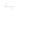
(a)

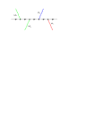
(b)

Figure 1: In an elastic scattering process [Fig. (a)], the atom absorbs and emits a single photon, each of frequency $\omega_{\rm L}$. That is, the atom emits the photon at the same frequency as the driving laser frequency. In an inelastic scattering process [Fig. (b)], the atom absorbs and emits more than one photon. Laser frequency $\omega_{\rm L}$. The frequencies of the scattered photons are $\omega_{S}$ and $\omega_{t}$. For many-photon processes, the sum of the emitted photons equals the sum of the frequencies of the absorbed photons.

This entire formalism is not applicable to the case of a laser-driven atom in a strong monochromatic (laser) field, because many-photon processes play a central role in this regime. The quantum electrodynamic (QED) interaction would have to be considered in very high orders of perturbation theory, and this is not feasible in practice. One distinguishes between the coherently scattered radiation (whose frequency is equal to the driving frequency) and the incoherently scattered radiation, which results from the many-photon processes. For a strong laser field, the ratio of the incoherently scattered intensity to the coherently scattered intensity tends to infinity, i.e. the incoherent part of the atomic fluorescence dominates.

Because it is hopelessly complicated to try to resum the entire QED series of the many-photon interactions, one has to invoke a quantum statistical treatment which was developed in the 1960s and 1970s Rautian and Sobel’man (1962); Mollow (1969); Oliver et al. (1971); Baklanov (1973); yet as a considerable simplification, one may restrict the Hilbert space of the atom to a few essential states whose energies are close to resonance. For instance, we may consider a two-level system described by the Jaynes–Cummings model Jaynes and Cummings (1963), which is a classic textbook example for a dynamical atom-laser system, well-known in theoretical quantum optics Scully and Zubairy (1997). Due to the driving of the laser field, the atomic population undergoes Rabi oscillations. The population is driven periodically from the upper to the lower state and vice versa. The emission spectrum of this process with a strong driving field is known as the Mollow spectrum Mollow (1969); its well-known three-peak structure may easily be interpreted in terms of the so-called dressed states, which are as the eigenstates of the combined system of atom and driving laser field Cohen-Tannoudji (1975) in a second-quantized formalism. These states diagonalize the atom-field interaction in all orders of perturbation theory, yet in a truncated Hilbert space of the atom and within the so-called rotating-wave approximation. The construction of the dressed states also implies approximations; but these are different from the ones carried out in a QED perturbative treatment of the problem and much more appropriate to the case of a strongly driven atom. Indeed, the terms left out in carrying out the approximations may easily be added later on and lead to perturbative corrections to the dressed-state energy levels. One natural question concerns the coupling of the laser-dressed atomic states to the modes of the vacuum field, i.e. the Lamb shift of the dressed states. The appropriate expansion parameters in this context are the fine-structure constant $\alpha$ and the coupling to the atomic nucleus $Z\alpha$. Furthermore, in a strong field, we may expand in powers of $\Gamma/\Omega$, where $\Gamma$ is the natural decay width of the upper level, and $\Omega$ is the Rabi frequency, and in $\Omega/\omega_{\rm R}$ and $\Delta/\omega_{\rm R}$, where $\omega_{\rm R}$ is the atomic resonance frequency Jentschura et al. (2003); Jentschura and Keitel (2004); Evers et al. . We hereby assume the Rabi frequency to be large as compared to the excited-state decay width but small compared to the atomic transition frequency.

We review initially the basic considerations that are relevant to the description of the Lamb shift of the laser-dressed states. For a strongly driven two-level atomic system, one may perform the analysis as outlined in Refs. Jentschura et al. (2003); Jentschura and Keitel (2004); Evers et al. , using a (two-level) rotating-wave dressed-state approximation as the starting point. This leads to a number of intensity- and detuning-dependent dynamic corrections to the generalized Rabi frequency which determines the Mollow sidebands. While the bare-state Lamb shift is recovered in the limit of a vanishing laser intensity, some of the corrections can only be understood if one carries out the analysis of the relativistic and radiative corrections in the dressed-state picture. Other atomic levels neglected in the initial construction of the laser-dressed states, as well as counter-rotating terms and quantum electrodynamic effects are taken into account perturbatively and lead to corrections which may be expressed in terms of the expansion parameters $\alpha$, $Z\alpha$, $\Gamma/\Omega$, $\Omega/\omega_{\rm R}$, and $\Delta/\omega_{\rm R}$. In this article, we consider a slight generalization of this scheme based on a laser-driven hydrogenic $1S$–$3P$ transition where the $3P$ state may decay spontaneously into the metastable $2S$-state. In the stationary state, a large percentage of the atomic population is trapped in the $2S$ state, and the fluorescence is not very intense. However, this should not be an obstacle for an experiment provided a suitable intensity-stabilized light source is available, and we demonstrate here that it is possible to generalize the treatment of the radiative laser-dressed relativistic and radiative corrections to multi-level systems.

Experimental work on the Mollow spectrum crucially depends on the availability of intense laser light sources because the Mollow side spectrum is only visible under these conditions (see also Sec. 3.1.2 of Mollow (1981)), and only if the Doppler shift is essentially eliminated, which implies the necessity of a collimated atomic beam. The first experimental confirmations of the Mollow theory have been achieved in Refs. Hartig and Walther (1973); Schuda et al. (1974); Walther (1975); Wu et al. (1975); Grove et al. (1975); Hartig et al. (1976); Gibbs and Venkatesan (1976); Citron et al. (1977); Grove et al. (1977).

In this article, we use rationalized Gaussian natural units with $\hbar=\epsilon_{0}=c=1$. The work is organized as follows: In Sec. II, we consider two basic phenomena which are crucial to an understanding of the interaction of an atom with a quantized field: (i) the nonrelativistic part of the self-energy in Sec. II.1, and (ii) the dynamic (AC) Stark shift of atomic energy levels in a laser field (Sec. II.2). Both of these effects are crucial for the treatment in Sec. III, where we analyze radiative corrections to the Mollow spectrum for hydrogenic $1S$–$3P_{j}$ transitions ($j=\nicefrac{{1}}{{2}},\nicefrac{{3}}{{2}}$) in detail. In Sec. III.1, we provide an overview of all corrections relevant to our analysis. This overview is related to the effects discussed in Secs. II.1 and II.2, but in addition, we take the opportunity to summarize a number of other effects (see also Ref. Evers et al. ) which contribute to the radiative modifications to the Mollow spectrum. These corrections fall naturally into two groups: the corrections within the two-level approximation (Sec. III.2), and those beyond this approximation (these result from the multi-level character of the system due to the additional spontaneous decay pathway $3P_{j}\to 2S\to 1S$, and are discussed in Sec. III.3). Explicit theoretical predictions for the $1S$–$3P_{j}$ transition at specific parameters for the Rabi frequency and the detuning are given in Sec. III.4. Finally, conclusions are drawn in Sec. IV.

II Basic Atom–Field Interactions

II.1 Derivation of the Nonrelativistic Part of the Self–Energy

The nonrelativistic part of the self-energy is the dominant contribution to the Lamb shift of (bare) atomic states due to the bound-state self-energy. One might, however, think that the energy shift of the electron due to the interaction with the vacuum modes is actually unobservable as it contributes to its mass. To resolve this question, it is necessary to consider the effects of the binding Coulomb field. The self-energy of the bound electron is then given by the bound-state self-energy shift minus the corresponding energy shift of a free electron. The difference is finite and leads to a small residual effect that shifts the bound-state energy levels in comparison to the results of the Dirac theory. In a strong laser field, the interaction with the vacuum modes is modified, because the electron interacts strongly with the driving laser field [see Fig. 2].

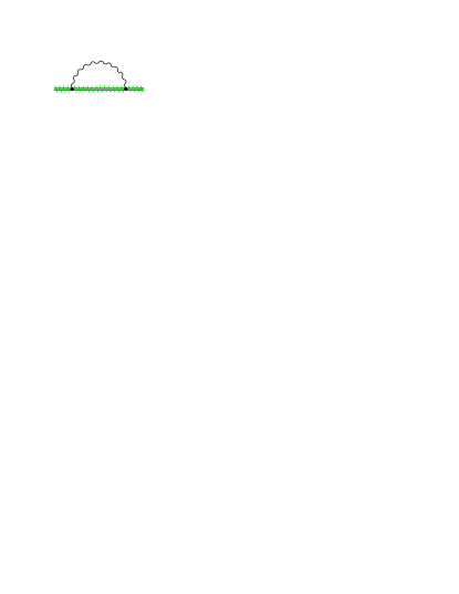
Figure 2: The laser-dressed self-energy involves an electron under the simultaneous influence of a strong driving laser field (zigzag line) and the binding Coulomb field of the atomic nucleus (double line). The formalism used in the analysis of this term is a generalization of the simple derivation discussed in Eq. (II.1).

However, an intuitive understanding can be gained from a simpler picture. Consider that in the usual quantum field theoretic formalism, the interaction is actually formulated in the interaction picture, which is why the operators acquire a time dependence. There is, however, no reason why one should not use the field operators in the time-independent Schrödinger representation. This procedure explicitly breaks the covariance, but one may satisfy oneself that Lorentz invariance appears to be broken in bound-state calculations already via the introduction of the manifestly noncovariant Coulomb interaction within the context of a vector potential. This means that one works in the rest frame of the atomic nucleus, which is assumed to be infinitely heavy in the non-recoil limit. In this context, one may use stationary as opposed to time-dependent perturbation theory, which simplifies the calculations.

The unperturbed Hamiltonian of the atom is

$${\mathcal{H}}_{\rm A}=\sum_{b}\,\omega_{b}\,|b\rangle\,\langle b|\,.$$ (1)

The normal-ordered Hamiltonian for the electromagnetic field is given by

$${\mathcal{H}}_{\rm F}=\sum_{\mbox{\boldmath$\scriptstyle k$}\lambda}\omega_{\mbox{\boldmath$\scriptstyle k$}}\,a^{+}_{\mbox{\boldmath$\scriptstyle k$}\lambda}\,a_{\mbox{\boldmath$\scriptstyle k$}\lambda}\,.$$ (2)

Therefore, we may assume an unperturbed atom$+$field Hamiltonian of the form

$${\mathcal{H}}_{0}={\mathcal{H}}_{\rm A}+{\mathcal{H}}_{\rm F}\,.$$ (3)

The Schrödinger-picture atom-field Hamiltonian in the dipole approximation and in the length gauge is given by (see Jentschura and Keitel (2004))

$${\mathcal{H}}_{\rm AF}\approx{\mathcal{H}}^{\rm(dip)}_{\rm length}=-q\,\mbox{\boldmath$x$}\cdot\mbox{\boldmath$E$}\,,$$ (4)

where $q$ is the physical charge of the electron, and the electric-dipole field operator is

$$\mbox{\boldmath$E$}=\sum_{\mbox{\boldmath$\scriptstyle k$}\lambda}\frac{1}{\sqrt{V}}\,\sqrt{\frac{\omega_{\mbox{\boldmath$\scriptstyle k$}}}{2}}\,\mbox{\boldmath$\epsilon$}_{\lambda}(\mbox{\boldmath$\scriptstyle k$})\,\left[a_{\mbox{\boldmath$\scriptstyle k$}\lambda}+a^{+}_{\mbox{\boldmath$\scriptstyle k$}\lambda}\right]\,.$$ (5)

Here, $a_{\mbox{\boldmath$\scriptstyle k$}\lambda}$ is the discrete-space annihilation operator for a photon with wave vector $k$ and polarization $\lambda\in\{1,2\}$. It is well known that the dominant contribution to the Lamb shift (self-energy) is due to virtual dipole transitions Eides et al. (2001). The first-order perturbation due to the dipole interaction Eq. (4) vanishes. The second-order perturbation (operators in the Schrödinger picture) can be written as

$$\delta E=\left<a,0\left|{\mathcal{H}}^{\rm(dip)}_{\rm length}\,\frac{1}{E_{a,0}-{\mathcal{H}}_{0}}\,{\mathcal{H}}^{\rm(dip)}_{\rm length}\right|a,0\right>\,,$$ (6)

where by $|a\rangle$ we denote the atomic reference state (not to be confused with the creation and annihilation operators!), and $|b,0\rangle$ stands for an atom-field state with the atom in state $|b\rangle$, and no photons. Also, we denote by ${\mathcal{H}}_{0}$ the unperturbed atom$+$field Hamiltonian in Eq. (3). The expression (6) involves a Green function which can be written as a sum over intermediate atom-field states. A priori, in the intermediate state, we have the atom in state $|b\rangle$ and an arbitrary Fock state of the photon field. However, a nonvanishing contribution is incurred only from those intermediate states with one and only one virtual photon. We denote the wave vector and the polarization state of this single virtual photon by $\mbox{\boldmath$k$}\lambda$.

The energy shift Eq. (6) can be written as

$$E_{\rm SE} =\sum_{b,\mbox{\boldmath$\scriptstyle k$}\lambda}\frac{\left<a,0\left|{\mathcal{H}}^{\rm(dip)}_{\rm length}\right|b,1_{\mbox{\boldmath$\scriptstyle k$}\lambda}\right>\,\left<b,1_{\mbox{\boldmath$\scriptstyle k$}\lambda}\left|{\mathcal{H}}^{\rm(dip)}_{\rm length}\right|a,0\right>}{E_{a}-(E_{b}+\omega_{\mbox{\boldmath$\scriptstyle k$}})}$$

$$=\sum_{b,\mbox{\boldmath$\scriptstyle k$}\lambda}\frac{q^{2}\,\omega_{\mbox{\boldmath$\scriptstyle k$}}}{2\,V}\,\frac{\left<a\left|\mbox{\boldmath$\epsilon$}_{\lambda}(\mbox{\boldmath$k$})\cdot\mbox{\boldmath$x$}\right|b\right>\,\left<b\left|\mbox{\boldmath$\epsilon$}_{\lambda}(\mbox{\boldmath$k$})\cdot\mbox{\boldmath$x$}\right|a\right>}{E_{a}-(E_{b}+\omega_{\mbox{\boldmath$\scriptstyle k$}})}$$

$$=\sum_{b,\mbox{\boldmath$\scriptstyle k$}}\frac{q^{2}\,\omega_{\mbox{\boldmath$\scriptstyle k$}}}{2\,V}\,\left(\delta^{ij}-\frac{k^{i}\,k^{j}}{\mbox{\boldmath$k$}^{2}}\right)\,\frac{\left<a\left|x^{i}\right|b\right>\,\left<b\left|x^{j}\right|a\right>}{E_{a}-(E_{b}+\omega_{\mbox{\boldmath$\scriptstyle k$}})}$$

$$\to q^{2}\,\sum_{b}\int\frac{{\rm d}^{3}k}{(2\pi)^{3}}\,\frac{k}{2}\,\delta^{T,ij}\,\frac{\left<a\left|x^{i}\right|b\right>\,\left<b\left|x^{j}\right|a\right>}{E_{a}-(E_{b}+k)}$$

$$=q^{2}\,\sum_{b}\int\frac{{\rm d}k\,k^{3}}{4\,\pi^{2}}\,\int\frac{{\rm d}\Omega_{\mbox{\boldmath$\scriptstyle k$}}}{4\,\pi}\,\delta^{T,ij}\,\frac{\left<a\left|x^{i}\right|b\right>\,\left<b\left|x^{j}\right|a\right>}{E_{a}-(E_{b}+k)}$$

$$=\frac{2\alpha}{3\,\pi}\,\int_{0}^{K}{\rm d}k\,k^{3}\,\left<a\left|x^{i}\,\frac{1}{E_{a}-({\mathcal{H}}_{\rm A}+k)}\,x^{i}\right|a\right>\,.$$ (7)

Here, in going from the third to the fourth line, we applied the discrete–continuum transition

$$\sum_{\mbox{\boldmath$\scriptstyle k$}}\frac{1}{V}\to\int\frac{{\rm d}^{3}k}{(2\pi)^{3}}\,,$$ (8)

which is based on counting the available free photon states in the normalization volume $V$. The transverse $\delta$ function is

$$\delta^{T,ij}=\delta^{ij}-\frac{k^{i}\,k^{j}}{\mbox{\boldmath$k$}^{2}}\,.$$ (9)

The integration of the virtual photon energy $k$ from $0$ to $K$ diverges for large $K$; a suitable subtraction of the first few terms in the asymptotic of the integrand for large $k$ leads to a finite result. The formalism used here is akin to the first calculation of the Lamb shift by Hans A. Bethe Bethe (1947), and it has recently found a more accurate interpretation in terms of methods for the treatment of Lamb shift corrections inspired by nonrelativistic quantum electrodynamics Caswell and Lepage (1986); Pachucki (1993). It has the advantage that it can be generalized also to other situations. Indeed, an application of this formalism to the laser-dressed states immediately yields the dominant self-energy corrections to their quasi-energies, as outlined in detail in Secs. 4.3 and 4.4 of Ref. Jentschura and Keitel (2004).

II.2 Derivation of the AC Stark Shift

We start from the second-quantized atom-laser Hamiltonian [see Eq. (4.10) of Jentschura and Keitel (2004)]:

$${\mathcal{H}}_{\rm L}=-q\,\mbox{\boldmath$x$}\cdot\mbox{\boldmath$E$}_{\rm L}\,,$$ (10)

where the laser-field operator is

$$\mbox{\boldmath$E$}_{\rm L}=\frac{1}{\sqrt{V}}\,\sqrt{\frac{\omega_{\rm L}}{2}}\,\mbox{\boldmath$\epsilon$}_{\rm L}\,\left[a_{\rm L}+a^{+}_{\rm L}\right]\,.$$ (11)

Here, $\mbox{\boldmath$\epsilon$}_{\rm L}=\hat{z}$ is the laser polarization. The second-order AC Stark shift is given by

$$E_{\rm AC}= \sum_{b}\left\{\frac{\left<a,n_{\rm L}\left|{\mathcal{H}}_{\rm L}\right|b,n_{\rm L}-1\right>\,\left<b,n_{\rm L}-1\left|{\mathcal{H}}_{\rm L}\right|a,n_{\rm L}\right>}{E_{a}+n_{\rm L}\,\omega_{\rm L}-(E_{b}+(n_{\rm L}-1)\,\omega_{\rm L})}\right.$$

$$\left.\quad+\frac{\left<a,n_{\rm L}\left|{\mathcal{H}}_{\rm L}\right|b,n_{\rm L}+1\right>\,\left<b,n_{\rm L}+1\left|{\mathcal{H}}_{\rm L}\right|a,n_{\rm L}\right>}{E_{a}+n_{\rm L}\,\omega_{\rm L}-(E_{b}+(n_{\rm L}+1)\,\omega_{\rm L})}\right\}$$

$$= \frac{q^{2}\,\omega_{\rm L}}{2\,V}\,\sum_{b}\left\{\frac{\left<a\left|z\right|b\right>\,\left<b\left|z\right|a\right>}{E_{a}-E_{b}+\omega_{\rm L}}\,n_{\rm L}\right.$$

$$\left.\quad+\frac{\left<a\left|z\right|b\right>\,\left<b\left|z\right|a\right>}{E_{a}-E_{b}-\omega_{\rm L}}\,(n_{\rm L}+1)\right\}$$

$$= q^{2}\,\frac{n_{\rm L}\,\omega_{\rm L}}{2\,V}\,\left\{\left<a\left|z\,\frac{1}{E_{a}-{\mathcal{H}}_{\rm A}+\omega_{\rm L}}\,z\right|a\right>\right.$$

$$\quad\left.+\left<a\left|z\,\frac{1}{E_{a}-{\mathcal{H}}_{\rm A}-\omega_{\rm L}}\,z\right|a\right>\right\}$$

$$\to 2\,\pi\,\alpha\,I\,\left\{\left<a\left|z\,\frac{1}{E_{a}-{\mathcal{H}}_{\rm A}+\omega_{\rm L}}\,z\right|a\right>\right.$$

$$\quad\left.+\left<a\left|z\,\frac{1}{E_{a}-{\mathcal{H}}_{\rm A}-\omega_{\rm L}}\,z\right|a\right>\right\}$$ (12)

In the transition “$\to$” to the continuum limit $V\to\infty$, which also implies a large number of laser photons $n_{\rm L}\to\infty$, we keep the ratio $n_{\rm L}/V\to$ constant, as it is this ratio which determines the laser intensity. Terms of order $1/V$, which lack the factor $n_{\rm L}$ in the numerator, may be neglected in this limit. In Eq. (II.2), $I$ denotes the laser intensity, and we remind the reader that natural units ($\hbar=c=\epsilon_{0}=1$) are being used. A generalization of the simple derivation described in Eq. (II.2) is relevant for the treatment of off-resonant corrections (see Sec. 4.6 of Jentschura and Keitel (2004)), which enter into the spectral decomposition of the propagator $1/(E_{a}-{\mathcal{H}}_{\rm A}-\omega_{\rm L})$.

III The $1S$–$3P_{j}$ Transition

III.1 A Summary of the Corrections to the Mollow Spectrum

We consider the Mollow spectrum shown in Fig. 3. The generalized Rabi frequency, which characterizes the position of the Mollow sideband peaks relative to the central peak (see Fig. 3), is given by

$$\Omega_{\rm R}=\sqrt{\Omega^{2}+\Delta^{2}}\,.$$ (13)

Here, the Rabi frequency is ($z$-polarization)

$$\Omega=\langle e|(-q\,z)|g\rangle\,{\mathcal{E}}_{\rm L}\,.$$ (14)

The expression $(\omega_{\rm L}/(2\,V))^{1/2}$ in Eq. (11) is the electric laser field ${\mathcal{E}}_{\rm L}$ per laser photon,

$${\mathcal{E}}_{\rm L}=\sqrt{\frac{\omega_{\rm L}}{2\,V}}\,.$$ (15)

Its matching with a macroscopic laser field can be done via

$$2\,\sqrt{n}\,\,{\mathcal{E}}_{\rm L}\approx 2\,\sqrt{n+1}\,\,{\mathcal{E}}_{\rm L}\to|\mbox{\boldmath${\mathcal{E}}$}|\,,$$ (16)

where ${\mathcal{E}}$ is the electric field amplitude of the laser in the convention ${\mbox{\boldmath$E$}}_{\rm L}(t)=\mbox{\boldmath${\mathcal{E}}$}\,\cos(\omega_{\rm L}\,t)$. In the following analysis, we will concentrate on the position of the sideband peaks in the Mollow spectrum, as it is a convenient observable. Thus we consider all corrections as modifications to the generalized Rabi frequency $\Omega_{\rm R}$ as defined in Eq. (13).

\psfrag{Int}[cc][cc][1][0]{Intensity [arb.u.]}\psfrag{Delta}[cc][cc][1][0]{$\Delta\>[\Gamma]$}\psfrag{OmegaR}[cc][cc][1][0]{$\Omega_{\textrm{R}}$}\includegraphics[height=113.81102pt,width=199.16928pt]{fig3.eps}

Figure 3: Mollow spectrum. The incoherently, inelastically scattered intensity is plotted against the detuning $\Delta=\omega_{\rm L}-\omega_{\rm R}$, where $\omega_{\rm L}$ is the laser frequency, and $\omega_{\rm R}$ is the atomic resonance frequency. The central elastic peak at zero detuning is not shown here. The displacement of the red and blue Mollow sideband peaks is $\Omega_{\rm R}$ as defined in Eq. (13).

It turns out that all corrections can be interpreted as modifications to either the Rabi frequency $\Omega$ or to the detuning $\Delta$ (see Sec. 3 of Evers et al. ). These corrections will be analyzed here for the $1S$–$3P_{j}$ transitions ($j=\nicefrac{{1}}{{2}},\nicefrac{{3}}{{2}}$) and depend on the total angular momentum $j$, i.e. they are different for the two fine-structure components of the $3P$ state. Our consideration of this transition is motivated in part by the recent advent of coherent-wave light sources for the hydrogen Lyman-$\alpha$ transition Eikema et al. (2001). This means that it is perhaps not unrealistic to consider the possibility of a coherent-wave light source for the $1S$–$3P_{j}$ transition. The modifications due to relativistic and radiative effects lead to the following modification in Eq. (13),

$$\Delta \to\Delta-\Delta^{(j)}_{\rm rad}\,,$$ (17)

$$\Omega \to\Omega\,\left(1+\hat{\Omega}_{\rm rad}^{(j)}\right)\,.$$ (18)

The $j$-dependent ($j=\nicefrac{{1}}{{2}},\nicefrac{{3}}{{2}}$) modifications are sums of the various contributions from the considered corrections:

$$\Delta^{(j)}_{\rm rad} =L^{(j)}_{\rm bare}+{\mathcal{B}}\,\Omega^{2}+{\mathcal{D}}_{\rm R}\,\Omega^{2}\,,$$ (19)

$$\hat{\Omega}_{\rm rad}^{(j)} ={\mathcal{A}}_{j}-{\mathcal{C}}_{j}-{\mathcal{E}}_{j}-{\mathcal{F}}-{\mathcal{S}}\,,$$ (20)

where all terms are explained in Sec. III.2 below. For the moment, we will only remark that the corrections to the detuning other than the bare Lamb shift vanish in the limit of a negligible laser intensity, i.e. in the limit $\Omega\to 0$, as it should be. Likewise, the relative modification $\hat{\Omega}_{\rm rad}^{(j)}$ of the Rabi frequency has a vanishing influence on the Mollow spectrum for small laser intensity because in this case, the quantity $\Omega$ itself tends to zero. The corrected formula for the Mollow sideband peaks in the two-level subsystem $\{1S,3P_{j}\}$,

$$\Omega_{\rm R}\to\Omega^{(j)}_{\mathcal{C}}\,,$$ (21)

then reads Evers et al.

$$\Omega^{(j)}_{\mathcal{C}}=\sqrt{\Omega^{2}\cdot\left(1+{\hat{\Omega}_{\rm rad}^{(j)}}\right)^{2}+\left(\Delta-{\Delta^{(j)}_{\rm rad}}\right)^{2}}\,.$$ (22)

In view of Eqs. (19) and (20), the radiative corrections to the detuning lead to a spin-dependent dynamic Lamb shift of the Mollow sidebands

$$\delta\overline{\omega}_{\pm}^{(j)}=\pm\left[\Omega^{(j)}_{\mathcal{C}}\,\left(1+\hat{\Omega}_{\rm multi}\right)\,-\Omega_{\rm R}\right]\,,$$ (23)

where the multiplicative modification $(1+\hat{\Omega}_{\rm multi})$ summarizes the effect of the additional intermediate atomic levels in a multi-level configuration (see Sec. III.3 below). This spin-dependent laser-dressed Lamb shift depends on two parameters which may be dynamically adjusted: the Rabi frequency and the detuning. From the two-dimensional manifold spanned by the Rabi frequency and the detuning, we have picked up one particular parameter combination in Sec. III.4 below.

III.2 Corrections Within the Two–Level Approximation

First, we treat the corrections to the detuning listed in Eq. (19). All corrections summarized here are discussed in detail in Evers et al. .

Bare Lamb shift: This correction concerns the term $L^{(j)}_{\rm bare}$ in Eq. (19) and is due to the Lamb shift of the atomic bare states caused mainly by self-energy corrections due to interaction of the atom with the surrounding vacuum field. The result is

$$L_{\rm bare}^{(j)} = L_{3P_{j}}-L_{1S}\,.$$ (24)

For the Lamb shift of the 3P states, we take the data published in Ref. Jentschura et al. (1997),

$$L_{3P_{\nicefrac{{1}}{{2}}}} =-3473.75(3)\>{\rm kHz},$$ (25)

$$L_{3P_{\nicefrac{{3}}{{2}}}} =4037.75(3)\>{\rm kHz}\,.$$ (26)

The $1S$ Lamb shift is given by Pachucki and Jentschura (2003)

$$L_{1S}=8172811(32)\>{\rm kHz}\,.$$ (27)

Bloch-Siegert shifts. This is the correction term ${\mathcal{B}}\,\Omega^{2}$ in Eq. (19), which is spin-independent to a good approximation Evers et al. . Essentially, the correction is caused by counter-rotating atom-field interaction term given by $\mathcal{H}^{({\rm CR})}_{\rm L}=g_{\rm L}\left(a^{+}_{\rm L}|e\rangle\langle g|+a_{\rm L}|g\rangle\langle e|\right)$ (see also Sec. 3 of Evers et al. and Sec. 4.5 of Jentschura and Keitel (2004)). We only present the result here, which reads

$${\cal B}=\frac{1}{\omega_{\rm R}}+{\mathcal{O}}(\Delta/\omega_{\rm L}^{2},\Omega/\omega_{\rm L}^{2})\,.$$ (28)

Off-resonant radiative corrections. Here, we are concerned with the term ${\mathcal{D}}_{\rm R}\,\Omega^{2}$ in Eq. (19). The derivation is outlined in Sec. 4.6 of Jentschura and Keitel (2004) and follows the ideas outlined in Sec. II.2. The result for this spin-independent term is (for the notation see Sec. 3 of Ref. Evers et al. )

$${\cal D}_{\rm R}=\frac{1}{\omega_{\textrm{R}}}\>5.202(3)\,.$$ (29)

We now turn our attention to the various relativistic and radiative corrections to the Rabi frequency listed in Eq. (20).

${\mathcal{E}}_{j}$ - Relativistic corrections to the dipole-moment. The evaluation of this spin-dependent correction to the transition dipole-moment requires the use of the relativistic wave functions Swainson and Drake (1991a, b), see Sec. 3 of Evers et al. . The result is

$${\mathcal{E}}_{\nicefrac{{1}}{{2}}} =(Z\alpha)^{2}\,\left(\frac{17}{24}-\ln 2+\frac{1}{2}\,\ln 3\right)\,,$$ (30a)

$${\mathcal{E}}_{\nicefrac{{3}}{{2}}} =(Z\alpha)^{2}\,\left(\frac{5}{24}-\frac{3}{4}\,\ln 2+\frac{1}{2}\,\ln 3\right)\,.$$ (30b)

Field-configuration dependent correction. This is the ${\mathcal{F}}$-term in Eq. (20). In evaluating this correction, we assume that the atom is placed in a standing-wave field, at an anti-node of the electric field, which implies also that the magnetic field can be neglected to a very good approximation. We are concerned with a field that is polarized along the $z$-direction, but whose magnitude is not constant in the propagation direction The correction may be evaluated using the long-wavelength QED Hamiltonian introduced in Pachucki (2004) (see also Sec. 3 of Evers et al. ). The result reads

$${\cal F}=\frac{1}{27}\>(Z\alpha)^{2}\,.$$ (31)

Higher-order corrections (in $\Omega$, $\Delta$) to the laser-dressed self-energy. This correction, which leads to the ${\mathcal{C}}_{j}$–term in Eq. (20), follows from an analysis of the Feynman diagram in Fig. 2. The correction has been analyzed in detail in Jentschura et al. (2003) and in Sec. 4.4 of Jentschura and Keitel (2004). The result is

$$\mathcal{C}_{j}=\alpha(Z\alpha)^{2}\>\frac{10}{9\pi}\>\left(\ln[(Z\alpha)^{-2}]-2\pm 2\right)\,,$$ (32)

where the spin-dependent constant term remains to be evaluated. We present here an estimate for this term ($-2\pm 2$); this estimate is based on the considerations outlined in Sec. 3 of Evers et al. .

Radiative correction to the dipole moment. This spin-dependent correction is given by the ${\mathcal{A}}_{j}$-term in Eq. (20). The leading logarithmic term, however, is spin-independent and given by the action of the radiative local potential

$$\Delta V_{\rm lamb}=\frac{4}{3}\>\alpha(Z\alpha)^{2}\>\ln[(Z\alpha)^{-2}]\>\frac{\delta^{(3)}(\mbox{\boldmath$r$})}{m^{2}}$$ (33)

on the $1S$ state,

$$\delta d^{(\rm log)}=\left<3P\left|z\,\left(\frac{1}{E-H}\right)^{{}^{\prime}}\Delta V_{{\rm lamb}}({\mbox{\boldmath$r$}})\right|1S\right>\,.$$ (34)

Note that the radiative potential in Eq. (33) is local, i.e. proportional to a Dirac-delta-function, such that the corresponding correction to the $3P$ wave function vanishes. The result for the spin-independent logarithmic correction is

$${\cal A}_{j}=\frac{\alpha\,(Z\alpha)^{2}}{\pi}\, \left\{\left[\frac{55}{27}+\frac{4}{3}\,\ln\left(\frac{3}{2}\right)\right]\,\ln[(Z\alpha)^{-2}]\right.$$

$$\left.\qquad-5.2\pm 5.2\right\}\,,$$ (35)

where we estimate the constant term according to the considerations outlined in Evers et al. .

${\mathcal{S}}$ - Corrections to the secular approximation. These are corrections of higher-order in $(\Gamma/\Omega)$ to the expression for the incoherent resonance fluorescence spectrum, see Eq. (2.64) of Jentschura and Keitel (2004). The result is

$${\cal S}=\frac{1}{2}\>\left(\frac{\Gamma}{\Omega}\right)^{2}+{\mathcal{O}}\left(\frac{\Delta^{2}\Gamma^{2}}{\Omega^{4}}\right)\,.$$ (36)

III.3 Beyond the Two–Level Approximation: Corrections Due to the Intermediate $2S$–Level

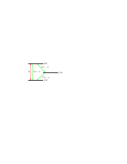
Figure 4: Relevant level scheme of the hydrogen atom. The upper state $3P$ decays via two channels to the ground state $1S$; the dominant channel is the direct decay, while the second channel involves the intermediate $2S$ state. Energy differences are not drawn to scale.

Going beyond the two-level approximation, the upper $3P$ state decays via two decay channels as shown in Fig. 4. The dominant decay chanel is the direct decay to the $1S$ state; the other channel involves the $2S$ state as intermediate state. The branching ratios are (see also Bethe and Salpeter (1957), p. 266)

$$A(3P\to 2S) =0.2245\times 10^{8}\,\,{\rm s}^{-1}\,,$$ (37a)

$$A(3P\to 1S) =1.6725\times 10^{8}\,\,{\rm s}^{-1}\,.$$ (37b)

Qualitatively, the system dynamics is as follows: We assume the atom to be in the ground state when it enters the interaction region with the laser field. On the timescale $A(3P\to 1S)^{-1}$, the atom reaches a quasi-stationary state within the two-level subspace $(1S,3P)$. At this point, the fluorescence light of the atom is well described within the above two-level approximation. Then, on the slower timescale $A(3P\to 2S)^{-1}$, the atom reaches its true steady state. In this stationary state, most of the population is trapped in the metastable $2S$ state; but still the atom emits some fluorescence light whose spectrum deviates from the two-level Mollow spectrum due to the third atomic state as outlined in Ref. Evers and Keitel (2002). In particular, the additional decay channel via the intermediate $2S$ state induces a relative shift of the Mollow sidebands as defined in Eq. (23) given by ($\Omega=1000\,\Gamma$, $\Delta=50\,\Gamma$)

$$\hat{\Omega}_{\rm multi}=6.3\times 10^{-7}\,.$$ (38)

In the following, we include this shift as an additional error, as in an experiment involving a beam of atoms both the two-level and the three-level spectra would be observed simultaneously. It should, however, be noted that the two-level spectrum would clearly dominate the experimental outcome, as the intensity of the three-level spectrum is very low due to the trapping of the population in the $2S$ state. Therefore, in the final results Eqs. (39, 40), the error induced by the additional atomic state is given separately.

III.4 Explicit Values for the $1S$–$3P_{1/2}$ and $1S$–$3P_{3/2}$ Transition

We consider the example $\Omega=1000\,\Gamma$, $\Delta=50\,\Gamma$, but with parameters adjusted for the $1S$–$3P_{j}$ transition (cf. Evers et al. ). The total correction is [see Table III.4 and Eqs. (23) as well as (38)]

$$\delta\overline{\omega}_{\pm}^{(\nicefrac{{1}}{{2}})}=1612394(33)(18)\>\textrm{kHz}$$ (39)

for the $1S$–$3P_{\nicefrac{{1}}{{2}}}$ transition and

$$\delta\overline{\omega}_{\pm}^{(\nicefrac{{3}}{{2}})}=1610305(33)(18)\>\textrm{kHz}$$ (40)

for the $1S$–$3P_{\nicefrac{{3}}{{2}}}$ transition. Here, the first bracket denotes the uncertainty arising from the uncertainties of the individual correction terms as listed in Tab. III.4, while the second bracket corresponds to the uncertainty due to the additional decay channel via the $2S$ state, see Eqs. (23, 38). Note that the results Eqs. (39,40) deviate slightly from the sum of the respective corrections in Tab. III.4, as there the shifts are evaluated individually.

Shift	1$S_{\nicefrac{{1}}{{2}}}\leftrightarrow$ 3$P_{\nicefrac{{1}}{{2}}}$ [kHz]	1$S_{\nicefrac{{1}}{{2}}}\leftrightarrow$ 3$P_{\nicefrac{{3}}{{2}}}$ [kHz]
$\delta\overline{\omega}^{\rm(Lamb)}_{+,j}$	$1613618(11)$	$1611093(11)$
$\delta\overline{\omega}^{\rm(BS)}_{+}$	$-3.025(1)$	$-3.025(1)$
$\delta\overline{\omega}^{\rm(OR)}_{+}$	$-62.91(4)$	$-62.91(4)$
$\delta\overline{\omega}^{\rm(R)}_{+,j}$	$-799.16(4)$	$-336.63(2)$
$\delta\overline{\omega}^{\rm(F)}_{+}$	$-52.434(3)$	$-52.434(3)$
$\delta\overline{\omega}^{\rm(C)}_{+,j}$	$-29(6)$	$-29(6)$
$\delta\overline{\omega}^{\rm(TDM)}_{+,j}$	$66(17)$	$66(17)$
$\delta\overline{\omega}^{(S)}_{+}$	$-13.29(4)$	$-13.29(4)$

Table 1: Summary of all individual energy shifts due to the various discussed corrections. These are all corrections to the Rabi frequency which follow from the analysis outlined in Sec. III.2, i.e. within the two-level approximation. For corrections which are beyond this approximation, see Sec. III.3.

IV Conclusions

In this article, we have analyzed the relativistic and radiative corrections to the stationary-state quasi-energies in a hydrogenic multi-level $1S$-$3P_{\nicefrac{{1}}{{2}}}$-$2S$ configuration. We demonstrate that it is possible to obtain theoretical predictions including the corrections which are beyond the two-level approximation (see Secs. III.2 and III.3, respectively). Explicit predictions for the case $\Omega=1000\,\Gamma$, $\Delta=50\,\Gamma$ are provided in Eqs. (39) and (40).

The modification of the Lamb shift in a dressed environment (i.e., a strong laser field) is complementary to other “dressed” situations like a cavity. Indeed, the Lamb shift in a cavity has received considerable attention in the past two decades, both theoretically as well as experimentally Barton (1970, 1987a, 1987b); Lütken and Ravndal (1985); Heinzen and Feld (1987); Sandoghdar et al. (1992); Sukenik et al. (1993); Brune et al. (1994); Nakajima et al. (1997). Also, one should take the occasion to mention that laser-dressed states have been used in many experiments on the Mollow-related phenomena, especially dressed states involving Rydberg levels. One of the ‘classic’ experimental setups in the field involves a maser tuned near resonance to a transition between two Rydberg states, which provides a strong driving field, as well as a microwave cavity whose eigenmode is also close to the resonance. There are three frequencies relevant to the problem: (i) the frequency of the driving field, (ii) the atomic resonance frequency (corresponding to the transition between Rydberg states), and (iii) the eigenmode of the cavity. It is well known that spontaneous emission can be enhanced if the cavity eigenmode frequency is equal to a Mollow sideband Zhu et al. (1988). The modifications of the cavity-induced spontaneous emission are well described by the optical master equation Agarwal et al. (1993), and good agreement between theory and experiment is obtained Agarwal et al. (1993); Lange and Walther (1993). For example, in Ref. Lange et al. (1996), the authors describe an experiment in which a two-photon transition between dressed states is observed in a driven microwave cavity. The atomic beam consists of ${}^{85}{\rm Rb}$ atoms excited to the $53{}^{2}{\rm P}_{3/2}$ state, and a maser is tuned near, but not on resonance to the transition to the $53{}^{2}{\rm S}_{1/2}$ state. When the detuning $\Delta$ is adjusted so that $\Delta=\pm\Omega_{\rm R}/2$, the otherwise dominant one-photon decay is suppressed, and the atom decays via emission of two photons into the cavity mode, under simultaneous absorption of a photon from the laser mode. The third photon is necessary in order to ensure angular momentum conservation in the electric dipole transition. Consequently, a further natural ground for an extension of the ideas outlined here would be to consider the laser-dressed Lamb shift in the additionally modified environment of a cavity.

In general, our approach is concerned with atomic physics; yet the analysis requires the techniques of quantum field theory. Approximate answers can be obtained for realistic situations by simply applying the results of the asymptotic-state formalism Gell-Mann and Low (1951); Sucher (1957) to the quantities that are of relevance to the dynamical process. However, as demonstrated here and in Jentschura et al. (2003); Jentschura and Keitel (2004); Evers et al. , there exist some small residual dynamic effects which can only be understood if one uses a picture in which the dynamics is treated in full. An experimental investigation of the laser-dressed Lamb shift, which depends on the laser intensity and the detuning, would require an accurate measurement of a (stabilized) laser intensity, which is problematic; other experimental issues include the Doppler effect, which must be controlled by using a well-collimated atomic beam Hartig et al. (1976). Yet, the intriguing consequences of the theoretical predictions may warrant this effort. Recent progress in heterodyne measurements of the resonance fluorescence of single ions Höffges et al. (1997a, b) may indicate that ultimately, achieving high accuracy in the measurement of the fluorescence spectra will rather depend on technical questions than on fundamental theoretical limitations.