Entanglement production in Quantized Chaotic Systems

Abstract

Quantum chaos is a subject whose major goal is to identify and to investigate different quantum signatures of classical chaos. Here we study entanglement production in coupled chaotic systems as a possible quantum indicator of classical chaos. We use coupled kicked tops as a model for our extensive numerical studies. We find that, in general, presence of chaos in the system produces more entanglement. However, coupling strength between two subsystems is also very important parameter for the entanglement production. Here we show how chaos can lead to large entanglement which is universal and describable by random matrix theory (RMT). We also explain entanglement production in coupled strongly chaotic systems by deriving a formula based on RMT. This formula is valid for arbitrary coupling strengths, as well as for sufficiently long time. Here we investigate also the effect of chaos on the entanglement production for the mixed initial state. We find that many properties of the mixed state entanglement production are qualitatively similar to the pure state entanglement production. We however still lack an analytical understanding of the mixed state entanglement production in chaotic systems.

1. Introduction

Entanglement is a unique quantum phenomenon which can be observed in a system consists of at least two subsystems. In case of an entangled system even if we know the exact state of the system, it is not possible to assign any pure state to the subsystems and that leads to the well-known unique quantum correlations which exists even in spatially well separated pairs of subsystems. This phenomenon was first discussed by Schrödinger to point out the nonclassicality implied by the quantum mechanical laws  [?]. This remarkable feature of quantum mechanics has recently been identified as a resource in many areas of quantum information theory including quantum teleportation  [?], superdense coding  [?] and quantum key distribution  [?]. Moreover, entanglement is also a key ingredient of all the proposed quantum algorithms which outperform their classical counterparts  [?,?].

Quantum mechanical study of classically chaotic systems is the subject matter of ‘quantum chaos’  [?,?]. A major challenge of quantum chaos is to identify quantum signatures of classical chaos. Various signatures have been identified, such as the spectral properties of the generating Hamiltonian  [?], phase space scarring  [?], hypersensitivity to perturbation  [?], and fidelity decay  [?], which indicate presence of chaos in underlying classical system. Recent studies have shown that entanglement in chaotic systems can also be a good indicator of the regular to chaotic transition in its classical counterpart  [?,?,?,?,?,?,?,?,?,?,?,?]. A study of the connections between chaos and entanglement is interesting because the two phenomena are prima facie uniquely classical and quantum, respectively. This is definitely an important reason to study entanglement in chaotic systems. Moreover, presence of chaos has also been identified in some realistic model of quantum computers  [?].

In this paper, we have investigated entanglement production in coupled chaotic systems. We have used coupled kicked tops as a model for our whole study. We have considered the entanglement production for both chaotic and regular cases. Moreover, we have also considered the effect of different coupling strengths on entanglement production. Most of the earlier studies have considered the effect of chaos on entanglement production for the case of initially pure state of the overall system. A basic assumption of these studies is that the initial state of the overall system is completely known. However, in many of the realistic scenarios, we do not have a complete knowledge of the state of a quantum system. For instance, when a quantum system interacts with its surroundings, it is not possible to know the exact state of the system. We may only express the state of the system as statistical mixture of different pure states, and that is a mixed state. In this paper we have also studied mixed state entanglement production in chaotic systems.

This paper is organized as follows. In the next section we discuss about classical and quantum properties of two coupled kicked tops, our primary model. Then we have defined the measures of both pure and mixed state entanglement. Finally, we have concluded this section with a discussion on the initial states (both pure and mixed) used here. In Sec.3., we present the numerical results on the entanglement production in coupled kicked tops for different single top dynamics and also for different coupling strengths. Here we have studied entanglement production for both pure and mixed initial state. In Sec.4., we derive the statistical universal bound on entanglement using random matrix theory (RMT). We also derive an approximate formula, based on RMT, to explain the entanglement production in coupled strongly chaotic systems. Finally, we summarize in Sec.5.

2. Preliminaries

2.1 Coupled kicked tops

1 Quantum top

The single kicked top is characterized by an angular momentum vector ${\bf J}=(J_{x},J_{y},J_{z})$, where these components obey the usual commutation rules. The Hamiltonian of the single top is given by  [?]

$$H(t)=\frac{\pi}{2}J_{y}+\frac{k}{2j}J_{z}^{2}\sum_{n=-\infty}^{n=+\infty}\,\delta(t-n).$$ (1)

The first term describes free precession of the top around $y$ axis with angular frequency $\pi/2$, and the second term is due to periodic $\delta$-function kicks. The second term is torsion about $z$ axis by an angle proportional to $J_{z}$, and the proportionality factor is a dimensionless constant $k/2j$. Now the Hamiltonian of the coupled kicked tops can be written, following Ref.  [?], as

$${\cal H}(t)=H_{1}(t)+H_{2}(t)+H_{12}(t),$$ (2)

where

$$H_{i}(t) \equiv \frac{\pi}{2}J_{y_{i}}+\frac{k_{1}}{2j}J_{z_{i}}^{2}\sum_{n}\,\delta(t-n)$$ (4)

$$H_{12}(t) \equiv \frac{\epsilon}{j}J_{z_{1}}J_{z_{2}}\sum_{n}\,\delta(t-n),$$ (5)

where $i=1,2$. Here $H_{i}(t)$’s represent the Hamiltonians of the individual tops, and $H_{12}(t)$ is the coupling between the tops via spin-spin interaction with a coupling strength $\epsilon/j$. Corresponding time evolution operator, defined in between two consecutive kicks, is given by

$$U_{T}=U_{12}^{\epsilon}(U_{1}\otimes U_{2})=U_{12}^{\epsilon}[(U_{1}^{k}U_{1}^{f})\otimes(U_{2}^{k}U_{2}^{f})],$$ (6)

where the different terms are given by,

$$U_{i}^{f}\equiv\exp\left(-i\frac{\pi}{2}J_{y_{i}}\right),\,U_{i}^{k}\equiv\exp\left(-i\frac{k}{2j}J_{z_{i}}^{2}\right),\,U_{12}^{\epsilon}\equiv\exp\left(-i\frac{\epsilon}{j}J_{z_{1}}J_{z_{2}}\right)$$ (7)

and as usual $i=1,2$.

2 Classical top

The classical map corresponding to the coupled kicked tops can be obtained from the quantum description with the Heisenberg picture in which the angular momentum operators evolve as

$${\bf J}_{n+1}=U_{T}^{\dagger}{\bf J}_{n}U_{T}.$$ (8)

Explicit form of this angular momentum evolution equation for each component of the angular momentum is presented in Ref. [?]. We now proceed by rescaling the angular momentum operator as $(X_{i},Y_{i},Z_{i})\equiv(J_{x_{i}},J_{y_{i}},J_{z_{i}})/j$, for $i=1,2$. The commutation relations satisfied by the components of this rescaled angular momentum vector as follow : $[X_{i},Y_{i}]=iZ_{i}/j,[Y_{i},Z_{i}]=iX_{i}/j$ and $[Z_{i},X_{i}]=iY_{i}/j$. Therefore, in $j\rightarrow\infty$ limit, components of this rescaled angular momentum vector will commute and become classical $c$-number variables. In this large-$j$ limit, we obtain the classical map corresponding to coupled kicked top as  [?]:

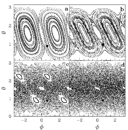
Figure  1.: Phase space pictures of the single top, corresponding to different parameter values, are presented. (a) $k=1.0$. Phase space is mostly covered by the regular region. (b) $k=2.0$. The phase space is still very much regular, but now a thin stochastic layer can be observed at the separatrix. (c) $k=3.0$. The phase space is truly mixed type. Few regular elliptic islands are visible inside the chaotic region. (d) $k=6.0$. The phase space is almost covered by the chaotic region with few tiny elliptic islands. The solid circle $(\bullet)$ is the point at which we will construct the initial wave packet during our study of the pure state entanglement production

$$X_{1}^{\prime} = Z_{1}\cos\Delta_{12}+Y_{1}\sin\Delta_{12},$$ (10)

$$Y_{1}^{\prime} = -Z_{1}\sin\Delta_{12}+Y_{1}\cos\Delta_{12},$$ (11)

$$Z_{1}^{\prime} = -X_{1},$$ (12)

$$X_{2}^{\prime} = Z_{2}\cos\Delta_{21}+Y_{2}\sin\Delta_{21},$$ (13)

$$Y_{2}^{\prime} = -Z_{2}\sin\Delta_{21}+Y_{2}\cos\Delta_{21},$$ (14)

$$Z_{2}^{\prime} = -X_{2},$$ (15)

where

$$\Delta_{12}\equiv kX_{1}+\epsilon X_{2}~{}~{}\mbox{and}~{}~{}\Delta_{21}\equiv kX_{2}+\epsilon X_{1}.$$ (16)

In the limit $\epsilon\rightarrow 0$, the classical map for the coupled kicked tops decouple into the classical map for two single tops. The classical map for one such uncoupled top can be written as

$$X^{\prime} = Z\cos kX+Y\sin kX$$ (18)

$$Y^{\prime} = -Z\sin kX+Y\cos kX$$ (19)

$$Z^{\prime} = -X.$$ (20)

It is clear from the above expression that the variables $(X,Y,Z)$ lie on the sphere of radius unity, i.e. $X^{2}+Y^{2}+Z^{2}=1$. Consequently, we can parameterize the dynamical variables in terms of the polar angle $\theta$ and the azimuthal angle $\phi$ as $X=\sin\theta\,\cos\phi,Y=\sin\theta\,\sin\phi,$ and $Z=\cos\theta$. In Fig. 1, we have presented the phase space diagrams of the single top for different values of the parameter $k$. For $k=1.0$, as shown in Fig.1(a), the phase space is mostly covered by regular orbits, without any visible stochastic region. Our initial wave packet, marked by a solid circle at the coordinate $(0.89,0.63)$, is on the regular elliptic orbits. As we further increase the parameter, regular region becomes smaller. Fig.1(b) is showing the phase space for $k=2.0$. Still the phase space is mostly covered by the regular region, but now we can observe a thin stochastic layer at the separatrix. In this case, the initial wave packet is on the separatrix. For the change in the parameter value from $k=2.0$ to $k=3.0$, there is significant change in the phase space. At $k=3.0$, shown in Fig.1(c), the phase space is of a truly mixed type. The size of the chaotic region is now very large with few regular islands. At this parameter value, the initial wave packet is inside the chaotic region. Fig.1(d) is showing the phase space for $k=6.0$. Now the phase space is mostly covered by the chaotic region, with very tiny regular islands. Naturally, our initial wave packet is in the chaotic region.

2.2 Measures of entanglement

1 Pure state

Entanglement measure for a system consisting of two subsystems (bipartite) is well defined if overall state of the system is in a pure state. In this case subsystem von Neumann entropy, i.e. von Neumann entropy of the reduced density matrices (RDMs), is a measure of entanglement. If there is no entanglement among the two subsystems, then the RDMs will correspond to density matrices of pure states and hence the subsystem von Neumann entropy will vanish. Otherwise, in case of entanglement, a non-zero value of the subsystem von Neumann entropy will be a measure of entanglement among the two subsystems.

Let us assume that the state space of a bipartite quantum system is ${\cal H}={\cal H}_{1}\otimes{\cal H}_{2}$, where $\mbox{dim}\,{\cal H}_{1}=N\leq\mbox{dim}\,{\cal H}_{2}=M$, and $\mbox{dim}\,{\cal H}=d=NM$. If $\rho=\sum_{i}p_{i}|\phi_{i}\,\rangle\langle\phi_{i}|$ is an ensemble representation of an arbitrary state in ${\cal H}$, the entanglement of formation is found by minimizing $\sum_{i}p_{i}E\left(|\phi_{i}\,\rangle\right)$ over all possible ensemble realizations. Here $E$ is the von Neumann entropy of the RDM of the state $|\phi_{i}\rangle$ belonging to the ensemble, i.e. its entanglement. For pure states $|\psi\rangle$ there is only one unique term in the ensemble representation and the entanglement of formation is simply the von Neumann entropy of the RDM.

The two RDMs of any bipartite pure state $|\psi\rangle$ are $\rho_{1}=\mbox{Tr}_{2}(|\psi\rangle\langle\psi|)$ and $\rho_{2}=\mbox{Tr}_{1}(|\psi\rangle\langle\psi|)$. The Schmidt decomposition of $|\psi\rangle$ is the optimal representation in terms of a product basis and is given by

$$|\psi\rangle=\sum_{i=1}^{N}\,\sqrt{\lambda}_{i}|\phi_{i}^{(1)}\rangle|\phi_{i}^{(2)}\rangle,$$ (21)

where $0<\lambda_{i}\leq 1$ are the (non-zero) eigenvalues of either RDMs and the vectors are the corresponding eigenvectors. The von Neumann entropy $S_{V}$ is the entanglement $E(|\psi\rangle)$ is given by

$$S_{V}=-\mbox{Tr}_{l}(\rho_{l}\ln\rho_{l})=-\sum_{i=1}^{N}\,\lambda_{i}\ln(\lambda_{i})\,\,;\,\,l=1,2.$$ (22)

The von Neumann entropy can only be calculated in the eigenbasis of the RDMs due to the presence of logarithmic function in its definition. Therefore it is not easy to calculate this measure unless one has some information of the eigenvalues of the RDMs. Consequently linearized version of the von Neumann entropy, called linear entropy, has also become a popular measure of entanglement. This measure of entanglement is defined as

$$S_{R}=1-\mbox{Tr}_{l}\rho_{l}^{2}=1-\sum_{i=1}^{N}\,\lambda_{i}^{2}\,\,;~{}l=1,2.$$ (23)

The linear entropy can be calculated without knowing the eigenvalues of the RDMs, because $\mbox{Tr}_{l}\rho_{l}^{2}$ is equal to the summation of absolute square of all the elements of RDMs. However, strictly speaking, the linear entropy is not a true measure of entanglement, rather it is a measure of mixedness of the subsystems which increases with entanglement among the two subsystems. Therefore, the linear entropy can be considered as an approximate measure of entanglement.

2 Mixed state

A major issue related to the study of the mixed state entanglement is lack of unique measure of entanglement. Probably this issue has discouraged any work related to the mixed state entanglement production in chaotic systems. Recently Vidal and Werner  [?] have proposed a computable measure of entanglement called Log-negativity following Peres’ criterion of separability  [?]. We use this measure to characterize mixed state entanglement production in chaotic systems. Basic idea of this measure is very simple and straightforward to state.

A most general form of a separable bipartite mixed state is given by

$$\rho=\sum_{i}\,p_{i}\,\rho_{i}^{(1)}\otimes\rho_{i}^{(2)},$$ (24)

where the positive weight factors $p_{i}$ satisfy $\sum_{i}\,p_{i}=1$, $\rho_{i}^{(1)}$ and $\rho_{i}^{(2)}$ are density matrices for the two subsystems. We can construct a matrix $\rho^{T_{2}}$ from $\rho$ by taking transpose only over second subspace, i.e.

$$\rho^{T_{2}}=\sum_{i}\,p_{i}\,\rho_{i}^{(1)}\otimes\left(\rho_{i}^{(2)}\right)^{T}.$$ (25)

This partial transpose operation is definitely not a unitary operation, but $\rho^{T_{2}}$ is still Hermitian. The transposed matrices $\left(\rho_{i}^{(2)}\right)^{T}$ are positive matrices, and hence they are legitimate density matrices. Consequently, if $\rho$ is separable, $\rho^{T_{2}}$ is a positive matrix. This is also true for $\rho^{T_{1}}$. In general, this is a necessary condition of separability.

Log-negativity measures the degree to which $\,\rho^{T_{2}}\,\left(\mbox{or}\,\rho^{T_{1}}\right)$ fails to be positive. If $\rho$ is an entangled state, then $\rho^{T_{2}}$ may have some negative eigenvalues. The Log-negativity is logarithm of the sum of absolute value of the negative eigenvalues of $\rho^{T_{2}}$ which vanishes for unentangled state. It can be shown by simple algebraic manipulation that the sum of absolute value of all the negative eigenvalues of $\rho^{T_{2}}$ is linearly related to the sum of absolute value of all the eigenvalues of $\rho^{T_{2}}$. Therefore, the Log-negativity measure $E_{N}(\rho)$ can be defined as

$$E_{N}(\rho)=\ln\left(\sum_{i=1}^{d}|\lambda_{i}|\right)$$ (26)

where $d$ is the dimension of $\rho$.

2.3 Initial state

1 pure state

We use generalized SU$(2)$ coherent state or the directed angular momentum state  [?,?] as our initial state for the individual tops and this state is given in standard angular momentum basis $|j,m\rangle$ as

$$\langle j,m|\theta_{0},\phi_{0}\rangle=(1+|\gamma|^{2})^{-j}\gamma^{j-m}\,\sqrt{\left(\begin{array}[]{c}2j\\ j+m\end{array}\right)},$$ (27)

where $\gamma\equiv\exp(i\phi_{0})\tan(\theta_{0}/2)$. For the coupled kicked top, we take the initial state as the tensor product of the directed angular momentum state corresponding to individual top, i.e.,

$$|\psi(0)\rangle=|\theta_{0}^{(1)},\phi_{0}^{(1)}\rangle\,|\theta_{0}^{(2)},\phi_{0}^{(2)}\rangle,$$ (28)

where $(\theta_{0}^{(i)},\phi_{0}^{(i)})=(0.89,0.63)$ for $i=1,2$. This initial state is evolved under $U_{T}$ as $|\psi(n)\rangle=U_{T}^{n}|\psi(0)\rangle$ for different values of the parameter $k$ and for different coupling strength $\epsilon$, and the results are displayed in Fig. 2.

2 mixed state

In this case we have considered a very simple unentangled mixed state, where the initial state corresponding to first top is mixed and the same corresponding to the second top is pure. Mathematically we express this state as $\rho(0)=\rho_{1}(0)\,\otimes\,|\psi_{2}(0)\rangle\,\langle\psi_{2}(0)|$, where $\rho_{1}(0)$ is the initial mixed state of the first subsystem and $|\psi_{2}(0)\rangle$ is the initial pure state of the second subsystem. We take $|\psi_{2}(0)\rangle$ as a generalized $SU(2)$ coherent state as presented above in Eq.(27). The mixed state $\rho_{1}(0)$ is a combination of two such coherent states placed at two different points on the phase space, i.e.,

$$\rho_{1}(0)=p\,|\theta_{a0}^{(1)},\phi_{a0}^{(1)}\rangle\,\langle\theta_{a0}^{(1)},\phi_{a0}^{(1)}|+(1-p)\,|\theta_{b0}^{(1)},\phi_{b0}^{(1)}\rangle\,\langle\theta_{b0}^{(1)},\phi_{b0}^{(1)}|.$$ (29)

Here we choose $\bigl{(}\theta_{a0}^{(1)},\phi_{a0}^{(1)}\bigr{)}=(0.89,0.63)$ and $\bigl{(}\theta_{b0}^{(1)},\phi_{b0}^{(1)}\bigr{)}=(2.25,-0.63)$ in such a way that the dynamical properties of these points are similar for any value of $k$. For the second top, we choose $|\psi_{2}(0)\rangle=|\theta_{0}^{(2)}=0.89,\phi_{0}^{(2)}=0.63\rangle$. We only consider $p=1/2$ case, this means the contribution of each coherent state is same on the formation of $\rho_{1}(0)$. The initial mixed state $\rho(0)$ is evolved under $U_{T}$ as $\rho(n)=U_{T}^{n}\rho(0)U_{T}^{-n}$. We study the time-evolution of the Log-negativity measure for different $k$ and $\epsilon$, and the results are displayed in Fig. 3.

3. Numerical results

3.1 Pure state entanglement production

In Fig.2, we have presented our results for the entanglement production in coupled kicked tops for the spin $j=80$. As we go from top to bottom window, coupling strength is decreasing by a factor of ten. Top window corresponds to $\epsilon=10^{-2}$, middle window is showing the results for $\epsilon=10^{-3}$, and the bottom one corresponds to the case $\epsilon=10^{-4}$. For each coupling strengths, we have studied entanglement production for four different single top parameter values, whose corresponding classical phase space picture has already been shown in Fig.1.

1 Coupling $\epsilon=10^{-2}$

The entanglement production for this strong coupling strength has been presented in Fig.2(a). It shows that there exists a saturation of $S_{V}$ for the regular cases ($k=1.0$ and $k=2.0$), which are much less than the saturation value corresponding to strongly chaotic cases such as when $k=6.0$. The saturation value of $S_{V}$ for $k=6.0$ is a statistical bound $S_{V}=\ln(N)-\frac{1}{2}\simeq 4.57$ (where $N=2j+1=161$), which can be estimated analytically from RMT  [?], and we will discuss about this in the next section. However for $k=3.0$, corresponding to a mixed classical phase space, the saturation value of $S_{V}$ is less than the above mentioned statistical bounds, which indicates the influence of the regular regions. These distinct behaviors of the entanglement saturation can be understood from the underlying classical dynamics. For $k=1.0$, the initial unentangled state is the product of the coherent wave packet placed on some elliptic orbits of each top. Therefore, the evolution of this unentangled state under the coupled top unitary operators is restricted by those elliptic orbits. Finally, the wave packet spreads all over those elliptic orbits and the entanglement production reaches its saturation value. At $k=2.0$, the center of the initial coherent state is inside the separatrix. Therefore, in its time evolution, the spreading of the wave packet is restricted to be inside the separatrix region. Finally it spread over the whole separatrix region, and the entanglement production arrives at its saturation. At $k=3.0$ and $k=6.0$, the initial wave packets are inside the chaotic region. However, due to the smaller size of the chaotic region corresponding to the case of $k=3.0$ than the case corresponding to $k=6.0$, the wave packet can spread over less of the phase space for $k=3.0$ than $k=6.0$. Consequently, the saturation value of the entanglement production is less for $k=3.0$ than $k=6.0$.

Figure  2.: Time evolution of the von Neumann entropy in coupled kicked tops is presented for different coupling strengths and for different underlying classical dynamics. (a) $\epsilon=10^{-2}$. (b) $\epsilon=10^{-3}$. (c) $\epsilon=10^{-4}$. Solid line represents $k=1.0$, dotted line corresponds to $k=2.0$, dashed line is for $k=3.0$ and dash-dot line represents $k=6.0$.

2 Coupling $\epsilon=10^{-3}$

Let us now discuss the case of coupling strength $\epsilon=10^{-3}$, whose results are presented in Fig.2(b). For the non-chaotic cases ($k=1.0$ and $k=2.0$), the saturation value of the entanglement production is less than the entanglement saturation value observed in the stronger coupling case $(\epsilon=10^{-2})$. This is because, for weaker coupling case, the interaction between two subsystems is less and the individual subsystems behave more like isolated quantum systems. Similarly, for the strong chaos case $(k=6.0)$, the entanglement production is well short of the known statistical bound $\ln(N)-\frac{1}{2}$.

3 Coupling $\epsilon=10^{-4}$

The entanglement production for this very weak coupling strength has been presented in Fig.2(c). The entanglement production for the weakly coupled strongly chaotic system has recently been explained by perturbation theory  [?]. However, the formula presented in that work is only valid for short time. In the next section we have presented an approximate formula for the entanglement production in coupled strongly chaotic systems which is valid for sufficiently long time and for any arbitrary coupling strengths. This formula explains the entanglement production for the strongly chaotic case $(k=6.0)$. Here we have observed an interesting phenomenon that the entanglement production is much larger for the non-chaotic cases than the chaotic cases. Rather, we can say that, for weakly coupled cases, the presence of chaos in the systems actually suppresses entanglement production.

3.2 Mixed state entanglement production

In Fig.3, we have presented the Log-negativity measure $E_{N}(\rho)$ of the mixed state entanglement production for different individual top dynamics $(k=1.0,2.0,3.0,$ and $6.0)$ and for different coupling strengths.

1 Coupling $\epsilon=1.0$

Let us start the discussion with the case of strong coupling $\epsilon=1.0$, whose results are presented in Fig.3(a). This coupling strength is so strong that, irrespective of the individual top dynamics, the overall coupled system is chaotic. Therefore, the location of the initial state and the dynamics of the individual tops are irrelevant for the saturation of $E_{N}(\rho)$. Consequently, we have observed almost same saturation value of $E_{N}(\rho)$ for all the different individual top dynamics.

Figure  3.: Evolution of the Log-negativity measure (evolving under the coupled tops time evolution operator $U_{T}$). Solid lines and dotted lines are representing the results corresponding to the non-chaotic cases ($k=1.0$ and $k=2.0$, respectively). Dashed lines are representing the mixed case $(k=3.0)$ and dash-dot lines are showing the results for the strongly chaotic case $(k=6.0)$. (a) Representing the results for the stronger coupling strength $(\epsilon=1.0)$. (b) This window is showing the results for $\epsilon=0.1$. (c) This window is for $\epsilon=0.01$ case. (d) This window is showing the results for the weak coupling case $(\epsilon=0.001$).

2 Coupling $\epsilon=0.1$

The time evolution of $E_{N}(\rho)$ corresponding to $\epsilon=0.1$ is presented in Fig.3(b). For this coupling strength, we have observed that the saturation value of $E_{N}(\rho)$ for the non-chaotic cases $(k=1.0\,\mbox{and}\,k=2.0)$ are less than the saturation value corresponding to other two cases. These lower saturation values of $E_{N}(\rho)$ for the non-chaotic cases indicate the influence of the regular orbits on the mixed state entanglement production. We have also noticed for the non-chaotic cases that the saturation value of $E_{N}(\rho)$ is less than the saturation value observed in the stronger coupling case $(\epsilon=1.0)$. However, the saturation value of $E_{N}(\rho)$ corresponding to other two cases, $k=3.0$ and $k=6.0$, are almost equal to the previous case $(\epsilon=1.0)$.

3 Coupling $\epsilon=10^{-2}$

The mixed state entanglement production for the coupling strength $\epsilon=10^{-2}$ has been presented in Fig.3(c). Here again the saturation value of $E_{N}(\rho)$ corresponding to the non-chaotic cases are less than the other two cases. Moreover, due to the weaker coupling, the saturation value of $E_{N}(\rho)$ for the non-chaotic cases are less than the saturation value observed in the previous two cases of stronger coupling strengths $(\epsilon=1.0$ and $\epsilon=0.1)$. Here we have first time observed an interesting phenomenon that the magnitude of $E_{N}(\rho)$ corresponding to the non-chaotic cases are larger than the other two cases at least within a time interval $50\mathrel{\mathchoice{\lower 3.0pt\vbox{\halign{$\m@th\displaystyle\hfill#\hfil$\cr<\crcr\sim\crcr}}}{\lower 3.0pt\vbox{\halign{$\m@th\textstyle\hfill#\hfil$\cr<\crcr\sim\crcr}}}{\lower 3.0pt\vbox{\halign{$\m@th\scriptstyle\hfill#\hfil$\cr<\crcr\sim\crcr}}}{\lower 3.0pt\vbox{\halign{$\m@th\scriptscriptstyle\hfill#\hfil$\cr<\crcr\sim\crcr}}}}n\mathrel{\mathchoice{\lower 3.0pt\vbox{\halign{$\m@th\displaystyle\hfill#\hfil$\cr<\crcr\sim\crcr}}}{\lower 3.0pt\vbox{\halign{$\m@th\textstyle\hfill#\hfil$\cr<\crcr\sim\crcr}}}{\lower 3.0pt\vbox{\halign{$\m@th\scriptstyle\hfill#\hfil$\cr<\crcr\sim\crcr}}}{\lower 3.0pt\vbox{\halign{$\m@th\scriptscriptstyle\hfill#\hfil$\cr<\crcr\sim\crcr}}}}100$. However, the saturation value corresponding to the case of mixed phase space $(k=3.0)$ is still less than the saturation value corresponding to the chaotic case $(k=6.0)$.

4 Coupling $\epsilon=10^{-3}$

Finally, for the weak coupling strength $\epsilon=10^{-3}$, we have observed completely different behaviors of the evolution of $E_{N}(\rho)$ and these results are presented in Fig.3(d). For this coupling strength, $E_{N}(\rho)$ corresponding to the non-chaotic cases are always higher than the chaotic cases within our time of observation. These results imply that, in case of weak coupling, the presence of chaos in the system actually suppresses the entanglement production. This suppression of the entanglement production by chaos for the weak coupling case was also observed for the pure state entanglement production, which we have already discussed in the previous section.

4. Some analytical results

4.1 Random matrix estimation of the statistical bound on entanglement

In our numerical study of pure state entanglement production, we have observed a statistical bound on entanglement for the strongly coupled strongly chaotic top. An identical property has also been observed for the stationary states of coupled standard map  [?] which indicates its universality. The parameter values considered in our numerical study, the nearest neighbor spacing distribution of the eigenangles of $U_{T}$ is Wigner distributed, which is typical of of any quantized chaotic systems  [?,?]. Therefore, it is quite reasonable to expect that the statistical bound on entanglement can be estimated by random matrix modeling.

Figure  4.: Distribution of the eigenvalues of the RDMs of coupled kicked tops, averaged over all the eigenstates ($N=2j_{1}+1=33$). Solid curves correspond to the theoretical distribution function Eq.(31).

The two RDMs, corresponding to two subsystems, have the structure $A^{\dagger}A$ and $AA^{\dagger}$, where $A$ is a rectangular $N\times M$ matrix containing the vector components of the bipartite system. We have pointed out the distribution of the eigenvalues of these RDMs as  [?]

$$f(\lambda) = \frac{NQ}{2\pi}\frac{\sqrt{(\lambda_{\mbox{max}}-\lambda)(\lambda-\lambda_{\mbox{min}})}}{\lambda}$$ (30)

$$\lambda_{\mbox{min}}^{\mbox{max}} = \frac{1}{N}\left(1+\frac{1}{Q}\pm\frac{2}{\sqrt{Q}}\right),$$ (31)

where $\lambda\in[\lambda_{\mbox{min}},\lambda_{\mbox{max}}],\,Q=M/N,$ and $Nf(\lambda)\,d\lambda$ is the number of eigenvalues within $\lambda$ to $\lambda+d\lambda$. This has been derived under the assumption that both $M$ and $N$ are large. Note that this predicts a range of eigenvalues for the RDMs that are of the order of $1/N$. For $Q\neq 1$, the eigenvalues of the RDMs are bounded away from the origin, while for $Q=1$ there is a divergence at the origin. All of these predictions are seen to be borne out in numerical work with coupled tops.

Fig.4 shows how well the above formula fits the eigenvalue distribution of reduced density matrices corresponding to the eigenstates of the coupled tops. Time evolving states also have the same distribution. This figure also shows that the probability of getting an eigenvalue outside the range $[\lambda_{\mbox{min}},\lambda_{\mbox{max}}]$ is indeed very small. The sum in $S_{V}$ [see Eq.(22)] can be replaced by an integral over the density $f(\lambda)$:

$$S_{V}\sim-N\int_{\lambda_{\mbox{min}}}^{\lambda_{\mbox{max}}}\,f(\lambda)\lambda\ln\lambda\,d\lambda\equiv\ln(\gamma N)=\ln(N)+\ln(\gamma).$$ (32)

The integral in $\gamma$ can be evaluated to a generalized hypergeometric function and the final result is

$$\gamma=\frac{Q}{Q+1}\exp\left[\frac{Q}{2(Q+1)^{2}}~{}{{{}_{3}}F_{2}}\left\{1,1,\frac{3}{2};2,3;\frac{4Q}{(Q+1)^{2}}\right\}\right].$$ (33)

When the Hilbert space dimension of the subsystems are equal, that is $Q=1$, the above expression gives $\gamma=\exp(-\frac{1}{2})$, and therefore the corresponding $S_{V}$ is $\ln(N)-\frac{1}{2}$. This is the statistical bound on entanglement found in our numerical study. In another extreme case, when $M\gg N$, that is $Q\gg 1$, then $\gamma\sim 1$ and the corresponding $S_{V}$ is equal to its maximum possible value $[\ln(N)]$. Therefore, the analytical formulation based on RMT is able to explain the saturation behavior of quantum entanglement production very accurately.

4.2 Entanglement production in coupled strongly chaotic system

We have already mentioned that, due to the simpler form of the linear entropy $S_{R}$, it is easier to derive an approximate formula for its time evolution. Here we now present an analytical formalism for the time evolution of $S_{R}$ in coupled strongly chaotic systems. Let us start the formalism with the assumption that the initial state is a product state, given as $|\psi(0)\rangle=|\phi_{1}(0)\rangle\otimes|\phi_{2}(0)\rangle$, where $|\phi_{i}(0)\rangle$’s are the states corresponding to individual subsystems. In general, the time evolution operator of a coupled system is of the form $U=U_{\epsilon}U_{0}=U_{\epsilon}(U_{1}\otimes U_{2})$, where $U_{\epsilon}$ is the coupling time evolution operator and $U_{i}$’s are the time evolution operators of the individual subsystems. Furthermore, we have assumed $U_{\epsilon}=\exp(-i\epsilon H_{12})$ where $H_{12}=h^{(1)}\otimes h^{(2)}$, and $h^{(i)}$ are Hermitian local operators. Here we derive our formalism in the eigenbasis of $h^{(i)}$’s, i.e., $h^{(i)}|e_{\alpha}^{(i)}\rangle=e_{\alpha}^{(i)}|e_{\alpha}^{(i)}\rangle$, where $\{e_{\alpha}^{(i)},|e_{\alpha}^{(i)}\rangle\}$ are the eigenvalues and the corresponding eigenvectors of $h^{(i)}$.

The one step operation of $U$ on $|\psi(0)\rangle$ will give the time evolving state at time $n=1$, i.e., $|\psi(1)\rangle$. Now, at this time, we can determine the matrix elements of RDM corresponding to the first subsystem in the eigenbasis of $h^{(i)}$’s as

$$[\rho_{1}(1)]_{\alpha\beta}=\sum_{\gamma}\exp\left[-i\epsilon\left(e_{\alpha}^{(1)}-e_{\beta}^{(1)}\right)e_{\gamma}^{(2)}\right]\langle e_{\alpha}^{(1)},e_{\gamma}^{(2)}|\psi_{0}(1)\rangle\langle\psi_{0}(1)|e_{\beta}^{(1)},e_{\gamma}^{(2)}\rangle,$$ (34)

where $|\psi_{0}(1)\rangle$ is the time evolving state of the uncoupled system. We now assume that $|\psi_{0}(1)\rangle$ is a random vector, and consequently we can further assume that the components of $|\psi_{0}(1)\rangle$ are uncorrelated to the exponential term coming due to the coupling. Therefore, we have

$$[\rho_{1}(1)]_{\alpha\beta}\simeq\frac{1}{N}\,\bigl{[}\rho_{10}(1)\bigr{]}_{\alpha\beta}\,\sum_{\gamma}\,\exp\left[-i\epsilon\left(e_{\alpha}^{(1)}-e_{\beta}^{(1)}\right)\,e_{\gamma}^{(2)}\right],$$ (35)

Figure  5.: Evolution of the Linear entropy for the coupled strongly chaotic system is presented. The dotted line is the numerical results of the coupled kicked tops system. We choose $k=6.0$ for the first top and $k=6.1$ for the second top. The solid line is the theoretical estimation, given by Eq.

where $N$ is the Hilbert space dimension of the first subsystem and $\rho_{10}$ is the density matrix corresponding to the uncoupled top. If we follow same procedure for one more time step, then at $n=2$ we have

$$\bigl{[}\rho_{1}(2)\bigr{]}_{\alpha\beta}\simeq\frac{1}{N}|p(\epsilon)|^{2}\bigl{[}\rho_{10}(2)\bigr{]}_{\alpha\beta}\sum_{\gamma}\,\exp\left[-i\epsilon\left(e_{\alpha}^{(1)}-e_{\beta}^{(1)}\right)\right]$$ (37)

where

$$p(\epsilon)=\frac{1}{N^{2}}\sum_{\alpha,\beta}\exp\left(-i\epsilon\,e_{\alpha}^{(1)}\,e_{\beta}^{(2)}\right).$$ (38)

If we evolve the initial state for any arbitrary time $n$ and follow the similar procedure as described above, we get

$$\bigl{[}\rho_{1}(n)\bigr{]}_{\alpha\beta}=\frac{1}{N}|p(\epsilon)|^{2(n-1)}\bigl{[}\rho_{10}(n)\bigr{]}_{\alpha\beta}\sum_{\gamma}\,\exp\left[-i\epsilon\left(e_{\alpha}^{(1)}-e_{\beta}^{(1)}\right)\,e_{\gamma}^{(2)}\right].$$ (39)

It is now straightforward to calculate linear entropy from the above expression, and that is given as

$$S_{R}(n)\simeq 1-\frac{1}{N^{4}}|p(\epsilon)|^{4(n-1)}\sum_{\alpha,\beta}\sum_{\gamma,\delta}\exp\left[-i\epsilon\left(e_{\alpha}^{(1)}-e_{\beta}^{(1)}\right)\left(e_{\gamma}^{(2)}-e_{\delta}^{(2)}\right)\right].$$ (40)

For the coupled kicked tops $H_{12}=J_{z_{1}}\otimes J_{z_{2}}/j$. Therefore, for this particular system, the above formula would become in large $j$-limit as

$$S_{R}(n) \simeq 1-p(\epsilon)^{4(n-1)}\Biggl{[}\frac{2}{N}\left\{1+\frac{\mbox{Si}\bigl{(}2N\epsilon\bigr{)}}{\epsilon}\right\}-\left(\frac{1}{N\epsilon}\right)^{2}$$ (43)

$$\times\bigl{\{}1-\cos\bigl{(}2N\epsilon\bigr{)}\bigr{.}\Biggr{.}+\mbox{Ci}\bigl{(}2N\epsilon\bigr{)}\,-\,\ln\bigl{(}2N\epsilon\bigr{)}-\gamma\Biggl{.}\bigl{.}\bigr{\}}\Biggr{]}$$

where

$$p(\epsilon)\simeq\frac{2}{N}\left[1+\frac{1}{\epsilon}\mbox{Si}\left(\frac{N\epsilon}{2}\right)\right].$$ (44)

The functions Si and Ci are the standard sine-integral and cosine-integral function, respectively, while $\gamma=0.577216...$ is the Euler constant. In the above formulation we have not assumed, unlike the perturbation theory  [?], any particular order of magnitude of the coupling strength $\epsilon$.

In Fig.5, we have presented our numerical result of the linear entropy $(S_{R})$ production in the coupled tops where the individual tops are strongly chaotic. In the above formalism, we have not assumed any special symmetry property. Here we break permutation symmetry by taking two nonidentical tops with $k=6.0$ for the first top and $k=6.1$ for the second. Fig.5 demonstrates that how well our theoretical estimation, denoted by the solid curve, is valid for both weak and strong coupling strengths.

5. Summary

In this paper, our major goal was to study entanglement production in coupled chaotic system as a possible quantum indicator of classical chaos. We have used coupled kicked top as a model for our study. Single kicked top is a well studied model of both classical and quantum chaotic system. Therefore, it is easier for us to identify the effect of underlying classical dynamics on the entanglement production. We have studied entanglement production for different underlying classical dynamics of the individual top and also for different coupling strengths. Here we not only have considered entanglement production for the pure initial state, but we have also initiated the study of entanglement production in coupled chaotic systems for the mixed initial state. We have used Log-negativity, a recently proposed measure, to characterize mixed state entanglement production. In general, for both kind of initial states, entanglement production is higher for stronger chaotic cases. However, we have observed a saturation of entanglement production when individual tops are strongly chaotic and they are coupled strongly to each other. Coupling strength between two tops is also a crucial parameter for the entanglement production. For instance, when the coupling strength between two tops is very weak, we find higher entanglement production for sufficiently long time corresponding to non-chaotic cases. This is also a common property of both kind of initial states. We analytically estimated the above mentioned statistical bound on the pure state entanglement (saturation of entanglement production) using RMT. We have also derived an approximate formula, based again on the ideas of RMT, for the pure state entanglement production in coupled strongly chaotic system. This formula is applicable, unlike perturbation theory, to large coupling strengths and is also valid for sufficiently long time. We still do not have deeper analytical understanding of mixed state entanglement production in chaotic systems, an open problem that is related to the establishment of calculable measures of mixed state entanglement.

REFERENCES

- [1] E. Schrödinger, Proc. Cambridge Philos. Soc. 31, 555 (1935).
- [2] C. H. Bennett et al, Phys. Rev. Lett. 70, 1895 (1993).
- [3] C. H. Bennett and S. J. Wiesner, Phys. Rev. Lett. 69, 2881 (1992).
- [4] A. K. Ekert, Phys. Rev. Lett. 67, 661 (1991).
- [5] P. W. Shor, In Proceedings of the 35th Annual Symposium on Foundations of Computer Science, edited by S. Goldwasser (IEEE Computer Society, Los Alamitos, CA, 1994), p. 124.
- [6] L. K. Grover, Phys. Rev. Lett. 79, 325 (1997) ; 79, 4709 (1997) ; 80, 4329 (1998).
- [7] F. Haake, Quantum Signatures of Chaos, 2nd ed. (Springer-Verlag, Berlin, 2000).
- [8] H.-J. Stöckman, Quantum Chaos : an Introduction, (Cambridge University Press, Cambridge, 1999).
- [9] O. Bohigas, M. J. Giannoni, and C. Scmit, Phys. Rev. Lett. 52, 1 (1984).
- [10] E. Heller, Phys. Rev. Lett. 53, 1515 (1984).
- [11] R. Schack, G. M. D’Ariano, and C. M. Caves, Phys. Rev. E 50, 972 (1994).
- [12] A. Peres, Phys. Rev. A 30, 1610 (1984).
- [13] K. Furuya, M. C. Nemes, and G. Q. Pellegrino, Phys. Rev. Lett. 80, 5524 (1998).
- [14] P. A. Miller and S. Sarkar, Phys. Rev. E 60, 1542 (1999).
- [15] A. Lakshminarayan, Phys. Rev. E 64, 036207 (2001).
- [16] J. N. Bandyopadhyay and A. Lakshminarayan, Phys. Rev. Lett. 89, 060402 (2002).
- [17] J. N. Bandyopadhyay and A. Lakshminarayan, Phys. Rev. E 69, 016201 (2004).
- [18] A. Tanaka, H. Fujisaki, and T. Miyadera, Phys. Rev. E 66, 045201(R) (2002); H. Fujisaki, T. Miyadera, and A. Tanaka, Phys. Rev. E 67, 066201 (2003).
- [19] A. Lakshminarayan and V. Subrahmanyam, Phys. Rev. A 67, 052304 (2003).
- [20] A. Lahiri and S. Nag, Phys. Lett. A 318, 6 (2003).
- [21] A. J. Scott and C. M. Caves, J. Phys. A 36, 9553 (2003).
- [22] L. F. Santos, G. Rigolin, and C. O. Escober, Phys. Rev. A 69, 042304 (2004).
- [23] X. Wang, S. Ghose, B. C. Shanders, and B. Hu, Phys. Rev. E 70, 016217 (2004).
- [24] R. Demkowicz-Dobrzański and M. Kus, e-print quant-ph/0403232.
- [25] B. Georgeot and D. L. Shepelyansky, Phys. Rev. E 62, 3504 (2000) ; 62, 6366 (2000).
- [26] F. Haake, M. Kus, and R. Scharf, Z. Phys. B 65, 381 (1987).
- [27] G. Vidal and R. F. Werner, Phys. Rev. A 65, 032314 (2002).
- [28] A. Peres, Phys. Rev. Lett. 76, 1413 (1996).