Entanglement and majorization in (1+1)-dimensional quantum systems

Abstract

Motivated by the idea of entanglement loss along Renormalization Group flows, analytical majorization relations are proven for the ground state of $(1+1)$-dimensional conformal field theories. For any of these theories, majorization is proven to hold in the spectrum of the reduced density matrices in a bipartite system when changing the size $L$ of one of the subsystems. Continuous majorization along uniparametric flows is also proven as long as part of the conformal structure is preserved under the deformation and some monotonicity conditions hold as well. As particular examples of our derivations, we study the cases of the XX, Heisenberg and XY quantum spin chains. Our results provide in a rigorous way explicit proves for all the majorization conjectures raised by Latorre, L$\ddot{{\rm u}}$tken, Rico, Vidal and Kitaev in previous papers on quantum spin chains.

I Introduction

In the last few years, the emerging field of quantum information science chuang has developed tools and techniques for the analysis of quantum systems which have been proved to be useful in other fields of physics. The study of many-body Hamiltonians, quantum phase transitions, and the quantum correlations -or entanglement- that these systems develop, are examples of this interdisciplinary research. In fact, understanding entanglement has been realized as one of the most challenging and interesting problems in physics Pres .

Another interesting application of the tools of quantum information science has been the use of majorization theory maj in order to analyze the structure present in the ground state -also called vacuum- of some models along Renormalization Group (RG) flows (for a recent review on RG, see carteret ). Following this idea, Latorre et al. fine-grained proposed that irreversibility along RG flows may be rooted in properties of the vacuum only, without necessity of accessing the whole Hamiltonian of the system and its excited states. The vacuum of a theory may already have enough information in order to envisage irreversibility along RG trajectories. Such an irreversibility was casted into the idea of an entanglement loss along RG flows, which proceeded in three constructive steps for (1+1)-dimensional quantum systems: first, due to the fact that the central charge of a (1+1)-dimensional conformal field theory is in fact a genuine measure of the bipartite entanglement present in the ground state of the system VLRK02 ; korepin-cardy , there is a global loss of entanglement due to the c-theorem of Zamolodchikov ctheorem , which assures that the value of the central charge at the ultraviolet fixed point is bigger or equal than its value at the infrared fixed point ($c_{UV}\geq c_{IR}$); second, given a splitting of the system into two contiguous pieces, there is a monotonic loss of entanglement due to the monotonicity numerically observed for the entanglement entropy between the two subsystems along the flow, decreasing when going away from the critical fixed (ultraviolet) point; third, this loss of entanglement is seen to be fine-grained, since it follows from a very strict set of majorization ordering relations, which the eigenvalues of the reduced density matrix of the subsystems are numerically seen to perfectly obey. This last step motivated the authors of fine-grained to affirm that there was a fine-grained entanglement loss along RG flows rooted in properties of the vacuum, at least for (1+1)-dimensional quantum systems. In fact, a similar fine-grained entanglement loss had already been numerically observed by Vidal et al. in VLRK02 , for changes in the size of the bipartition described by the corresponding ground-state density operators, at conformally-invariant critical points.

In this work, we analytically prove the links between conformal field theory (CFT), RG and entanglement that were conjectured in the recent papers VLRK02 ; fine-grained for quantum spin chains. We develop, in the bipartite scenario, a detailed and analytical study of the majorization properties of the eigenvalue spectrum obtained from the reduced density matrices of the ground state for a variety of $(1+1)$-dimensional quantum models in the bulk. Our approach is based on infinitesimal variations of the parameters defining the model -magnetic fields, anisotropies- or deformations in the size of the block $L$ for one of the subsystems. We prove in these situations that there are strict majorization relations underlying the structure of the eigenvalues of the considered reduced density matrices or, as defined in fine-grained , there is a fine-grained entanglement loss. The result of our study is presented in terms of two theorems. On the one hand, we prove exact continuous majorization relations in terms of deformations of the size of the block $L$ that is considered. On the other hand, we are also able to prove continuous majorization relations as a function of the parameters defining the model. On top we also provide explicit analytical examples for models with a boundary based on previous work of Peschel, Kaulke and Legeza peschel1 .

This paper is structured as follows: in sec.II we remember the concepts of global, monotonous and fine-grained entanglement loss, as defined in fine-grained . In sec.III we analytically prove continuous majorization relations for any $(1+1)$-dimensional CFT when the size of the subsystem $L$ is changed, and give an example of a similar situation for the case of the XX-model with a boundary. In sec.IV we prove continuous majorization relations with respect to the flows in parameter space for $(1+1)$-dimensional quantum systems under perturbations which preserve part of the conformal structure of the partition function. Again, we support our result with the analysis of a similar situation for the Heisenberg and XY quantum spin chains with a boundary. Finally, sec.V collects the conclusions of our study. We also review in appendix A the definition of majorization and provide a lemma which will be used in our calculations.

II Global, monotonous and fine-grained entanglement loss

Consider the pure ground state (or vacuum) $|\Omega\rangle$ of a given physical system which depends on a particular set of parameters, and let us perform a bipartition of the system into two pieces $A$ and $B$. The density matrix for $A$, describing all the physical observables accessible to $A$, is given by $\rho_{A}={\rm tr}_{B}(|\Omega\rangle\langle\Omega|)$ -and analogously for $B$-. In this section we will focus our discussion on the density matrix for the subsystem $A$, so we will drop the subindex $A$ from our notation. Let us consider a change in one -for simplicity- of the parameters on which the resultant density matrix depends, say, parameter “$t$”, which can be either an original parameter of the system or the size of the region $A$. In other words, we make the change $\rho(t_{1})\rightarrow\rho(t_{2})$, where $t_{1}\neq t_{2}$. In order to simplify even more our discussion let us assume that $t_{2}>t_{1}$. We wish to understand how this variation of the parameter alters the inner structure of the ground state and, in particular, how does it modify the entanglement between the two parties $A$ and $B$. Because we are considering entanglement at two different points $t_{2}$ and $t_{1}$, we assume for simplicity that the entanglement between $A$ and $B$ is bigger at the point $t_{1}$ than at the point $t_{2}$, so we have an entanglement loss when going from $t_{1}$ to $t_{2}$.

Our characterization of this entanglement loss will progress through three stages, as in fine-grained , refining at every step the underlying ordering of quantum correlations. These three stages will be respectively called global, monotonous and fine-grained entanglement loss.

Global entanglement loss.-

The simplest way to quantify the loss of entanglement between $A$ and $B$ when going from $t_{1}$ to $t_{2}$ is by means of the entanglement entropy $S(\rho(t))=-{\rm tr}(\rho(t)\ln{\rho(t)})$. Since at $t_{2}$ the two parties are less entangled than at $t_{1}$, we have that

$$S(\rho(t_{1}))>S(\rho(t_{2}))\ ,$$ (1)

which is a global assessment between points $t_{2}$ and $t_{1}$. This is what we shall call global entanglement loss.

Monotonous entanglement loss.-

A more refined quantification of entanglement loss can be obtained by imposing the monotonicity of the derivative of the entanglement entropy when varying parameter “$t$”. That is, the condition

$$\frac{{\rm d}S}{{\rm d}t}<0$$ (2)

implies a stronger condition in the structure of the ground state under deformations of the parameter. This monotonic behavior of the entanglement entropy is what we shall call monotonous entanglement loss.

Fine-grained entanglement loss.-

When monotonous entanglement loss holds, we can wonder whether, in fact, it is the spectra of the underlying reduced density matrix the one that becomes more and more ordered as we change the value of the parameter. It is then natural to ask if it is possible to characterize the reordering of the density matrix eigenvalues along the flow beyond the simple entropic inequality discussed before and thereby unveil some richer structure. The finest notion of reordering when changing the parameter is then given by the monotonic majorization (see appendix A) of the eigenvalue distribution along the flow. If we call $\vec{\rho}(t)$ the vector corresponding to the probability distribution of the spectra arising from the density operator $\rho(t)$, then the condition

$$\vec{\rho}(t_{1})\prec\vec{\rho}(t_{2})\ ,$$ (3)

whenever $t_{2}>t_{1}$ will reflect the strongest possible ordering of the ground state along the flow. This is what we call fine-grained entanglement loss, and it is fine-grained since this condition involves a whole tower of inequalities to be simultaneously satisfied (see appendix A). In what follows we will see that this precise majorization condition will appear in different circumstances when studying $(1+1)$-dimensional quantum systems.

III Fine-grained entanglement loss with the size of the block in $(1+1)$-dimensional CFT

A complete analytical study of majorization relations for any $(1+1)$-dimensional conformal field theory (without boundaries) is presented in the bipartite scenario when the size of the considered subsystems changes, i.e., under deformations in the interval of the accessible region for one of the two parties. This size will be represented by the length $L$ of the space interval for which we consider the reduced density matrix $\rho_{L}$ after tracing out all the degrees of freedom corresponding to the rest of the universe. Our main result in this section can be casted into the following theorem:

Theorem: $\rho_{L}\prec\rho_{L^{\prime}}$ if $L\geq L^{\prime}$ for all possible $(1+1)$-dimensional CFT.

Proof:

Let $Z(\tau,\bar{\tau})=q^{-b}{\rm tr}(q^{(L_{0}+\bar{L}_{0})})$ be the partition function of a subsystem of size $L$ on a torus entropycft , where $q=e^{2\pi i\tau}$, $\tau=\frac{i\kappa}{\ln{(L/\epsilon)}}$ with $\kappa$ a positive constant, $\epsilon$ being an ultraviolet cut-off and $b\equiv(c+\bar{c})/24$ a combination of the holomorphic and antiholomorphic central charges that define the universality class of the model. The unnormalized density matrix $\rho_{L}$ can then be written as $\rho_{L}=q^{-b}q^{(L_{0}+\bar{L}_{0})}$, since $\rho_{L}$ can be understood as a propagator and $(L_{0}+\bar{L}_{0})$ is the generator of translations in time (dilatations in the conformal plane) entropycft . Furthermore, we have that

$${\rm tr}(q^{(L_{0}+\bar{L}_{0})})=1+n_{1}q^{\alpha_{1}}+n_{2}q^{\alpha_{2}}+\cdots\ ,$$ (4)

due to the fact that $(L_{0}+\bar{L}_{0})$ is diagonal in terms of highest-weight states $|h,\,\bar{h}\rangle$: $(L_{0}+\bar{L}_{0})|h,\,\bar{h}\rangle=(h+\bar{h})|h,\,\bar{h}\rangle$, with $h\geq 0$ and $\bar{h}\geq 0$; the coefficients $\alpha_{1},\alpha_{2},\ldots>0$, $\alpha_{i+1}>\alpha_{i}\ \forall i$ are related with the scaling dimensions of the descendant operators, and $n_{1},n_{2},\ldots$ are degeneracies. The normalized distinct eigenvalues of $\rho_{L}$ are then given by

$$\begin{split}\lambda_{1}&=\frac{1}{(1+n_{1}q^{\alpha_{1}}+n_{2}q^{\alpha_{2}}+\cdots)}\\ \lambda_{2}&=\frac{q^{\alpha_{1}}}{(1+n_{1}q^{\alpha_{1}}+n_{2}q^{\alpha_{2}}+\cdots)}\\ \vdots\\ \lambda_{l}&=\frac{q^{\alpha_{(l-1)}}}{(1+n_{1}q^{\alpha_{1}}+n_{2}q^{\alpha_{2}}+\cdots)}.\end{split}$$ (5)

Let us define $\tilde{Z}(q)\equiv{\rm tr}(q^{(L_{0}+\bar{L}_{0})})=(1+n_{1}q^{\alpha_{1}}+n_{2}q^{\alpha_{2}}+\cdots)$. The behavior of the eigenvalues in terms of deformations with respect to parameter $L$ follows from,

$$\frac{{\rm d}\tilde{Z}(q)}{{\rm d}L}=\frac{\tilde{Z}(q)-1}{q}\frac{{\rm d}q}{{\rm d}\ln{(L/\epsilon)}}\frac{{\rm d}\ln{(L/\epsilon)}}{{\rm d}L}\geq 0,$$ (6)

and therefore

$$\frac{{\rm d}\lambda_{1}}{{\rm d}L}=\frac{{\rm d}}{{\rm d}L}\left(\frac{1}{\tilde{Z}(q)}\right)\leq 0.$$ (7)

Because $\lambda_{1}$ is always the biggest eigenvalue $\forall L$, the first cumulant automatically satisfies continuous majorization when decreasing the size of the interval $L$. The variation of the rest of the eigenvalues $\lambda_{l}$, $l>1$, with respect to $L$ reads as follows:

$$\begin{split}&\frac{{\rm d}\lambda_{l}}{{\rm d}L}=\frac{{\rm d}}{{\rm d}L}\left(\frac{q^{\alpha_{(l-1)}}}{\tilde{Z}(q)}\right)\\ &=\frac{q^{\alpha_{(l-1)}-1}}{\tilde{Z}(q)}\left(\alpha_{(l-1)}-\frac{\tilde{Z}(q)-1}{\tilde{Z}(q)}\right)\frac{{\rm d}q}{{\rm d}L}.\end{split}$$ (8)

Let us focus on the second eigenvalue $\lambda_{2}$. Clearly two different situations can happen:

• if $\left(\alpha_{1}-\frac{\tilde{Z}(q)-1}{\tilde{Z}(q)}\right)\geq 0$, then since $\alpha_{(l-1)}>\alpha_{1}\ \forall l>2$, we have that $\left(\alpha_{(l-1)}-\frac{\tilde{Z}(q)-1}{\tilde{Z}(q)}\right)>0\ \forall l>2$, which in turn implies that $\frac{{\rm d}\lambda_{l}}{{\rm d}L}\geq 0\ \forall l\geq 2$. From this we have that the second cumulant satisfies

  $$\frac{{\rm d}(\lambda_{1}+\lambda_{2})}{{\rm d}L}=-\frac{{\rm d}}{{\rm d}L}\left(\sum_{l>2}\lambda_{l}\right)\leq 0\ ,$$ (9)

  thus fulfilling majorization. The same conclusion extends easily in this case to all the remaining cumulants, and therefore majorization is satisfied by the whole probability distribution.

• if $\left(\alpha_{1}-\frac{\tilde{Z}(q)-1}{\tilde{Z}(q)}\right)<0$, then $\frac{{\rm d}\lambda_{2}}{{\rm d}L}<0$, and therefore $\frac{{\rm d}(\lambda_{1}+\lambda_{2})}{{\rm d}L}<0$, so the second cumulant satisfies majorization, but nothing can be said from this about the rest of the remaining cumulants.

Proceeding with this analysis for each one of the eigenvalues we see that, if these are monotonically decreasing functions of $L$ then majorization is fulfilled for the particular cumulant under study, but since $\alpha_{i+1}>\alpha_{i}\ \forall i$ we notice that once the first monotonically increasing eigenvalue is found, majorization is directly satisfied by the whole distribution of eigenvalues, therefore $\rho_{L}\prec\rho_{L^{\prime}}$ if $L\geq L^{\prime}$. This proof is valid for all possible $(1+1)$-dimensional conformal field theories since it is based only on completely general assumptions. $\square$

III.1 Analytical finite-$L$ majorization for the critical quantum $XX$-model with a boundary

Let us give an example of a similar situation to the one presented in the previous theorem for the case of the quantum $XX$-model with a boundary, for which the exact spectrum of $\rho_{L}$ can be explicitly computed. The Hamiltonian of the model without magnetic field, is given by the expression

$$H=\sum_{n=1}^{\infty}(\sigma_{n}^{x}\sigma_{n+1}^{x}+\sigma_{n}^{y}\sigma_{n+1}^{y}).$$ (10)

The system described by the $XX$-model is critical since it has no mass gap. Taking the ground state and tracing out all but a block of $L$ contiguous spins, the density matrix $\rho_{L}$ describing this block can be written, in the large $L$ limit, as a thermal state of free fermions (see peschel1 ):

$$\rho_{L}=\frac{e^{-H^{\prime}}}{Z_{L}},$$ (11)

$Z_{L}$ being the partition function for a given $L$, $H^{\prime}=\sum_{k=0}^{L-1}\epsilon_{k}d^{{\dagger}}_{k}d_{k}$, with fermionic operators $d^{{\dagger}}_{k}$, $d_{k}$ and dispersion relation

$$\epsilon_{k}=\frac{\pi^{2}}{2\ {\rm ln}L}(2k+1)\ \ k=0,1,\ldots,L-1\ .$$ (12)

The eigenvalues of the density matrix $\rho_{L}$ can then be written in terms of non-interactive fermionic modes

$$\begin{split}\rho_{L}(n_{0},n_{1},\ldots,n_{L-1})&=\frac{1}{Z_{L}}e^{-\sum_{k=0}^{L-1}n_{k}\epsilon_{k}}\\ &=\rho_{L}(n_{0})\cdots\rho_{L}(n_{L-1})\ ,\end{split}$$ (13)

with $\rho(n_{\alpha})=\frac{1}{Z_{L}^{\alpha}}e^{-n_{\alpha}\epsilon_{\alpha}}$, where $Z_{L}^{\alpha}=(1+e^{-\epsilon_{\alpha}})$ is the partition function for the mode $\alpha$, and $n_{\alpha}=0,1$, $\forall\alpha$. It is worth noticing that the partition function of the whole block $Z_{L}$ can then be written as a product over the $L$ modes:

$$Z_{L}=\prod_{k=0}^{L-1}\left(1+e^{-\epsilon_{k}}\right)\ .$$ (14)

Once the density matrix of the subsystem is well characterized with respect to its size $L$, it is not difficult to prove that $\rho_{L}\prec\rho_{L^{\prime}}$ if $L\geq L^{\prime}$. In order to see this, we will fix the attention in the majorization within each mode and then we will apply the direct product lemma from appendix A for the whole subsystem. We initially have to observe the behavior in $L$ of the biggest probability defined by each individual distribution for each one of the modes, that is, $P^{\alpha}_{L}=1/Z^{\alpha}_{L}=(1+e^{-\epsilon_{\alpha}})^{-1}$, for $\alpha=0,1,\ldots,L-1$. It is straightforward to see that

$$\frac{{\rm d}P^{\alpha}_{L}}{{\rm d}L}=\frac{e^{-\epsilon_{\alpha}}}{\left(1+e^{-\epsilon_{\alpha}}\right)^{2}}\frac{{\rm d}\epsilon_{\alpha}}{{\rm d}L}<0\ ,$$ (15)

which implies that $P^{\alpha}_{L}$ decreases if $L$ increases $\forall\alpha$. This involves majorization within each mode $\alpha=0,1,\ldots,L-2$ when decreasing $L$ by one unit. In addition, we need to see what happens with the last mode $\alpha=L-1$ when the size of the system is reduced from $L$ to $L-1$. Because this mode disappears for the system of size $L-1$, its probability distribution turns out to be represented by the probability vector $(1,0)$, which majorizes any probability distribution of two components. Combining these results with the direct product lemma from appendix A, we conclude that this example for the quantum XX-model provides a similar situation for a model with a boundary to the one presented in our previous theorem.

IV Fine-grained entanglement loss along uniparametric flows in $(1+1)$-dimensional quantum systems

We study in this section strict continuous majorization relations along uniparametric flows, under the conditions of integrable deformations and monotonicity of the eigenvalues in parameter space. The main result of this section can be casted into the next theorem:

Theorem: consider a $(1+1)$-dimensional physical theory which depends on a set of real parameters $\vec{g}=(g_{1},g_{2},\ldots)$, such that

• there is a non-trivial conformal point $\vec{g}^{*}$, for which the model is conformally invariant

• the deformations from $\vec{g}^{*}$ in parameter space in the positive direction of a given unitary vector $\hat{e}$ preserve part of the conformal structure of the model, i.e., the eigenvalues of the reduced density matrices of the vacuum $\rho(\vec{g_{2}})$ are still of the form given in eq.(5) for values of the parameters $\vec{g}_{1}=\vec{g}^{*}+a\hat{e}$

• $\hat{e}\cdot\left(\vec{\nabla}_{\vec{g}}q(\vec{g})\right)\bigg{|}_{\vec{g_{1}}}\leq 0$, where $q(\vec{g})$ are the corresponding parameter-dependent conformal $q$-factors.

Then, away from the conformal point there is continuous majorization of the eigenvalues of the reduced density matrices of the ground state along the flow in the parameters $\vec{g}$ in the positive direction of $\hat{e}$, i.e.,

$$\begin{split}&\rho(\vec{g}_{1})\prec\rho(\vec{g}_{2}),\\ \vec{g}_{1}=\vec{g}^{*}+a\hat{e}&,\,\vec{g}_{2}=\vec{g}^{*}+a^{\prime}\hat{e},\,a^{\prime}\geq a.\end{split}$$ (16)

Proof.-

If the eigenvalues are assumed to be of the form given by eq.(5), then it is straightforward to see that $\hat{e}\cdot\left(\vec{\nabla}_{\vec{g}}\lambda_{1}(\vec{g})\right)\bigg{|}_{\vec{g_{1}}}\geq 0$, which assures that the first cumulant fulfills majorization. The rest of the analysis is completely equivalent to the one presented in the previous proof of the theorem in sec.III, which also proves this theorem. $\square$

The applicability of this theorem is based on the conditions we had to assume as hypothesis. Indeed, these conditions are naturally fulfilled by many interesting models. We now wish to illustrate this point with the analytical examples of similar situations for the Heisenberg and XY quantum spin chains with a boundary.

IV.1 Analytical majorization along the anisotropy flow for the Heisenberg quantum spin chain with a boundary

Consider the Hamiltonian of the Heisenberg quantum spin chain with a boundary

$$H=\sum_{n=1}^{\infty}\left(\sigma_{n}^{x}\sigma_{n+1}^{x}+\sigma_{n}^{y}\sigma_{n+1}^{y}+\Delta\sigma_{n}^{z}\sigma_{n+1}^{z}\right)\ ,$$ (17)

where $\Delta$ is the anisotropy parameter. This model is non-critical for $\Delta>1$ and critical at $\Delta=1$. From the pure ground state of the system, it is traced out half of it, getting an infinite-dimensional density matrix which describes half of the system ($N/2$ contiguous spins in the limit $N\rightarrow\infty$). The resulting reduced density matrix $\rho_{\Delta}$ can be written as a thermal density matrix of free fermions peschel1 , in such a way that its eigenvalues are given by

$$\rho_{\Delta}(n_{0},n_{1},\ldots,n_{\infty})=\frac{1}{Z_{\Delta}}e^{-\sum_{k=0}^{\infty}n_{k}\epsilon_{k}}\ ,$$ (18)

with dispersion relation

$$\epsilon_{k}=2k\ {\rm arcosh}(\Delta)\ ,$$ (19)

and $n_{k}=0,1$, for $k=0,1,\ldots,\infty$. The physical branch of the function ${\rm arcosh}(\Delta)$ is defined for $\Delta\geq 1$ and is a monotonic increasing function as $\Delta$ increases. On top, the whole partition function $Z_{\Delta}$ can be decomposed as an infinite direct product of the different free fermionic modes.

From the last equations, it is not difficult to see that $\rho_{\Delta}\prec\rho_{\Delta^{\prime}}$ if $\Delta\leq\Delta^{\prime}$. Fixing the attention in a particular mode $\alpha$, we evaluate the derivative of the biggest probability for this mode, $P^{\alpha}_{\Delta}=(1+e^{-\epsilon_{\alpha}})^{-1}$. This derivative is seen to be

$$\frac{{\rm d}P^{\alpha}_{\Delta}}{{\rm d}\Delta}=\frac{2\alpha}{(1+e^{-\epsilon_{\alpha}})^{2}\sqrt{\Delta^{2}-1}}>0\ ,$$ (20)

for $\alpha=1,2,\ldots\infty$ and $0$ for $\alpha=0$. It follows from this fact that all the modes independently majorize their respective probability distributions as $\Delta$ increases, with the peculiarity that the $0$th mode remains unchanged along the flow, being its probability distribution always $(\frac{1}{2},\frac{1}{2})$. The particular behavior of this mode is the responsible for the appearance of the “cat” state that is the ground state for large values of $\Delta$ (in that limit, the model corresponds to the quantum Ising model without magnetic field). These results, together with the direct product lemma from appendix A, make this example obey majorization along the flow in the parameter.

IV.2 Analytical majorization along uniparametric flows for the quantum $XY$-model with a boundary

Similar results to the one obtained for the Heisenberg model can be obtained as well for a more generic quantum spin chain. Let us consider the quantum $XY$-model with a boundary, as described by the Hamiltonian

$$H=-\sum_{n=1}^{\infty}\left((1+\gamma)\sigma_{n}^{x}\sigma_{n+1}^{x}+(1-\gamma)\sigma_{n}^{y}\sigma_{n+1}^{y}+2\lambda\sigma_{n}^{z}\right)\ ,$$ (21)

where $\gamma$ can be regarded as the anisotropy parameter and $\lambda$ as the magnetic field. The phase diagram of this model is shown in fig.(1), where it is seen that there exist different critical regions depending on the values of the parameters. Consider the ground state of this Hamiltonian of infinite number of spins, and trace out half of the system (if the size of the system is $N$, we trace out $N/2$ contiguous spins, and take the limit $N\rightarrow\infty$), for given values of $\lambda$ and $\gamma$. The resulting density matrix $\rho_{(\lambda,\gamma)}$ can be written as a thermal state of free fermions, and its eigenvalues are given by (see peschel1 ):

$$\rho_{(\lambda,\gamma)}(n_{0},n_{1},\ldots,n_{\infty})=\frac{1}{Z_{(\lambda,\gamma)}}e^{-\sum_{k=0}^{\infty}n_{k}\epsilon_{k}}\ ,$$ (22)

where $n_{k}=0,1$, and the single-mode energies $\epsilon_{k}$ are given by

$$\epsilon_{k}=\begin{cases}2k\epsilon\ ,&{\rm if}\ \lambda<1\\ (2k+1)\epsilon\ ,&{\rm if}\ \lambda>1\ ,\end{cases}$$ (23)

with $k=0,1,\ldots,\infty$. The parameter $\epsilon$ is defined by the relation

$$\epsilon=\pi\frac{I(\sqrt{1-x^{2}})}{I(x)}\ ,$$ (24)

$I(x)$ being the complete elliptic integral of the first kind

$$I(x)=\int_{0}^{\pi/2}\frac{d\theta}{\sqrt{1-x^{2}\sin^{2}(\theta)}}$$ (25)

and $x$ being given by

$$x=\begin{cases}(\sqrt{\lambda^{2}+\gamma^{2}-1})/\gamma\ ,&{\rm if}\ \lambda<1\\ \gamma/(\sqrt{\lambda^{2}+\gamma^{2}-1})\ ,&{\rm if}\ \lambda>1\ ,\end{cases}$$ (26)

with the condition $\lambda^{2}+\gamma^{2}>1$ (external region of the BM-circle BM ).

We note that the probability distribution defined by the eigenvalues of $\rho_{(\lambda,\gamma)}$ is the direct product of distributions for each one of the separate modes. Therefore, in order to study majorization we can focus separately on each one of these modes, in the same way as we already did in the previous examples. We wish now to consider our analysis in terms of the flows with respect to the magnetic field $\lambda$ and with respect to the anisotropy $\gamma$ in a separate way.

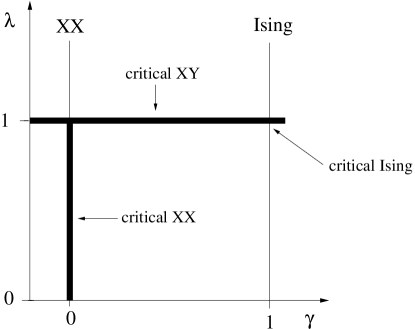
Figure 1: phase diagram of the quantum $XY$-model.

IV.2.1 Flow along the magnetic field $\lambda$

We consider in this subsection a fixed value of $\gamma$ while the value of $\lambda$ changes, always fulfilling the condition $\lambda^{2}+\gamma^{2}>1$. Therefore, at this point we can drop $\gamma$ from our notation. We separate the analysis of majorization for the regions $1<\lambda<\infty$ and $+\sqrt{1-\gamma^{2}}<\lambda<1$ for reasons that will become clearer during the example but that already can be realized just by looking at the phase space structure in fig.(1).

$1<\lambda<\infty$.-

We show that $\rho_{\lambda}\prec\rho_{\lambda^{\prime}}$ if $\lambda\leq\lambda^{\prime}$. In this region of parameter space, the biggest probability for the mode $\alpha$ is $P^{\alpha}_{\lambda}=(1+e^{-\epsilon_{\alpha}})^{-1}$, with

$$\epsilon_{\alpha}=(2\alpha+1)\pi\frac{I(\sqrt{1-x^{2}})}{I(x)}=(2\alpha+1)\epsilon\ ,$$ (27)

where $x=\gamma/(\sqrt{\lambda^{2}+\gamma^{2}-1})$. The variation of the biggest eigenvalue with respect to $\lambda$ is

$$\frac{{\rm d}P^{\alpha}_{\lambda}}{{\rm d}\lambda}=\frac{(2\alpha+1)e^{-(2\alpha+1)\epsilon}}{\left(1+e^{-(2\alpha+1)\epsilon}\right)^{2}}\frac{{\rm d}\epsilon}{{\rm d}\lambda}\ .$$ (28)

It is easy to see that

$$\begin{split}&\frac{{\rm d}\epsilon}{{\rm d}\lambda}=\frac{{\rm d}\epsilon}{{\rm d}x}\frac{{\rm d}x}{{\rm d}\lambda}\\ &=\frac{\pi}{I(x)}\left(\frac{{\rm d}I(\sqrt{1-x^{2}})}{{\rm d}x}-\left(\frac{I(\sqrt{1-x^{2}})}{I(x)}\right)\frac{{\rm d}I(x)}{{\rm d}x}\right)\frac{{\rm d}x}{{\rm d}\lambda}>0\ ,\end{split}$$ (29)

since both $\left(\frac{{\rm d}\epsilon}{{\rm d}x}\right)<0$ and $\left(\frac{{\rm d}x}{{\rm d}\lambda}\right)<0$. Therefore, $\frac{{\rm d}P^{\alpha}_{\lambda}}{{\rm d}\lambda}>0$ for $\alpha=0,1,\ldots,\infty$. This derivation shows mode-by-mode majorization when $\lambda$ increases. Combining this result with the direct product lemma from appendix A, we see that this example obeys majorization.

$+\sqrt{1-\gamma^{2}}<\lambda<1$.-

For this case, we show that $\rho_{\lambda}\prec\rho_{\lambda^{\prime}}$ if $\lambda\geq\lambda^{\prime}$. In particular, the probability distribution for the $0$th fermionic mode remains constant and equal to $(\frac{1}{2},\frac{1}{2})$, which brings a “cat” state for low values of $\lambda$. Similar to the latter case, the biggest probability for mode $\alpha$ is $P^{\alpha}_{\lambda}=(1+e^{-\epsilon_{\alpha}})^{-1}$, with

$$\epsilon_{\alpha}=2\alpha\pi\frac{I(\sqrt{1-x^{2}})}{I(x)}=2\alpha\epsilon\ ,$$ (30)

and $x=(\sqrt{\lambda^{2}+\gamma^{2}-1})/\gamma$. Its derivative with respect to $\lambda$ is

$$\frac{{\rm d}P^{\alpha}_{\lambda}}{{\rm d}\lambda}=\frac{2\alpha e^{-2\alpha\epsilon}}{\left(1+e^{-2\alpha\epsilon}\right)^{2}}\frac{{\rm d}\epsilon}{{\rm d}\lambda}\ .$$ (31)

It is easy to see that this time $\left(\frac{{\rm d}\epsilon}{{\rm d}\lambda}\right)<0$, and therefore $\frac{{\rm d}P^{\alpha}_{\lambda}}{{\rm d}\lambda}<0$ for $\alpha=1,2,\ldots,\infty$, which brings majorization individually for each one of these modes when $\lambda$ decreases. The mode $\alpha=0$ needs of special attention, from eq.(31) it is seen that $\frac{{\rm d}P^{\alpha=0}_{\lambda}}{{\rm d}\lambda}=0$, therefore the probability distribution for this mode remains constant and equal to $(\frac{1}{2},\frac{1}{2})$ all along the flow. This is a marginal mode that brings the system to a “cat” state that appears as ground state of the system for low values of $\lambda$. Notice that this peculiarity is rooted on the particular form of the dispersion relation given in equation (23), which is proportional to $2k$ instead of $2k+1$ for this region in parameter space. These results, together with the direct product lemma from appendix A, prove that this example fulfills also majorization.

IV.2.2 Flow along the anisotropy $\gamma$

In this subsection, the magnetic field $\lambda$ is fixed and the anisotropy $\gamma$ is the only free parameter of the model, always fulfilling $\lambda^{2}+\gamma^{2}>1$. Thus, at this point we can drop $\lambda$ from our notation. We will see that $\rho_{\gamma}\prec\rho_{\gamma^{\prime}}$ if $\gamma\geq\gamma^{\prime}$, in the two regions $1<\lambda<\infty$ and $+\sqrt{1-\gamma^{2}}<\lambda<1$. In particular, in the region $+\sqrt{1-\gamma^{2}}<\lambda<1$, the probability distribution for the $0$th fermionic mode remains constant and equal to $(\frac{1}{2},\frac{1}{2})$. Let us consider the biggest probability for the mode $\alpha$, $P^{\alpha}_{\gamma}=(1+e^{-\epsilon_{\alpha}})^{-1}$, with $\epsilon_{\alpha}=\omega\epsilon$, where

$$\omega=\begin{cases}2\alpha\ ,&{\rm if}\ \lambda<1\\ (2\alpha+1)\ ,&{\rm if}\ \lambda>1\ ,\end{cases}$$ (32)

and $\epsilon$ as defined in the preceding sections. It is easy to verify that

$$\frac{{\rm d}P^{\alpha}_{\gamma}}{{\rm d}\gamma}=\frac{\omega e^{-\omega\epsilon_{\alpha}}}{(1+e^{-\omega\epsilon_{\alpha}})^{2}}\frac{{\rm d}\epsilon}{{\rm d}x}\frac{{\rm d}x}{{\rm d}\gamma}<0$$ (33)

for $\alpha=0,1,\ldots,\infty$ if $\lambda>1$ and for $\alpha=1,2,\ldots,\infty$ if $\lambda<1$. The mode $\alpha=0$ for $\lambda<1$ needs of special attention: it is seen that $\frac{{\rm d}P^{\alpha=0}_{\lambda}}{{\rm d}\lambda}=0$, therefore the probability distribution for this mode remains constant and equal to $(\frac{1}{2},\frac{1}{2})$ all along the flow. These results, together with the direct product lemma from appendix A, show that this case also obeys majorization along the flow in the parameter.

V Conclusions

In this paper we have provided in a rigorous way explicit proves for all the majorization conjectures raised by Latorre, L$\ddot{{\rm u}}$tken, Rico, Vidal and Kitaev in previous papers on quantum spin chains fine-grained ; VLRK02 . In particular, we have developed a completely general proof of majorization relations underlying the structure of the vacuum with respect to the size of the block $L$ for all possible $(1+1)$-dimensional conformal field theories. An example of a similar situation has been given with the particular case of the XX-model with a boundary, for which the explicit calculation of the eigenvalues of the reduced density matrix can be performed. We have proven as well the existence of a fine-grained entanglement loss for $(1+1)$-dimensional quantum systems along uniparametric flows, regarded that perturbations in parameter space preserve part of the conformal structure of the partition function, and some monotonicity conditions hold as well. Again examples of similar situations have been provided by means of the Heisenberg and XY models with a boundary. Our results provide solid mathematical grounds for the existence of majorization relations along RG-flows underlying the structure of the vacuum of (1+1)-dimensional quantum spin chains.

Understanding the entanglement structure of the vacuum of $(1+1)$-dimensional models is a major task in quantum information science. For instance, spin chains like the ones described in the particular examples of this paper can be used as possible approximations to the complicated interactions that take place in the register of a quantum computer porras . Entanglement across a quantum phase transition has also an important role in quantum algorithm design, and in particular in quantum algorithms by adiabatic evolution orus1 . On top, the properties of quantum state transmission through spin chains are also intimately related to the entanglement properties present in the chain tobby . Consequently, our precise characterization of entanglement in terms of majorization relations should be helpful for the design of more powerful quantum algorithms and quantum state transmission protocols.

It would also be of interest trying to relate the results presented in this paper to possible extensions of the c-theorem ctheorem to systems with more than (1+1)-dimensions. While other approaches are also possible ignacio-forte , majorization may be a unique tool in order to envisage irreversibility of RG-flows in terms of properties of the vacuum only, and some numerical results in this direction have already been observed in systems of different dimensionality along uniparametric flows orus . New strict mathematical results could probably be achieved in these situations following the ideas that we have presented all along this work.

Acknowledgments: the author is grateful to very fruitful and enlightening discussions with J.I. Latorre, C. A. L$\ddot{{\rm u}}$tken, E. Rico and G. Vidal about the content of this paper, and also to H. Q. Zhou, T. Barthel, J. O. Fjaerestad and U. Schollwoeck for pointing an error in a previous version of this paper. Financial support from projects MCYT FPA2001-3598, GC2001SGR-00065 and IST-199-11053 is also acknowledged.

Note added: after completion of this paper a similar work appeared bcft in which entanglement and majorization are considered from the point of view of boundary conformal field theory, and where it was noticed that there was an error in the proof of the first theorem of a previous version of this paper. That error has been corrected in this new version.

Appendix A Lemmas on Majorization

This appendix includes the formal definitions of majorization maj as well as a lemma that is used along the examples presented in this work.

A.1 Definitions

Let $\vec{x}$, $\vec{y}\in\mathbb{R}^{N}$ be two vectors such that $\sum_{i=1}^{N}x_{i}=\sum_{i=1}^{N}y_{i}=1$, which represent two different probability distributions. We say that distribution $\vec{y}$ majorizes distribution $\vec{x}$, written $\vec{x}\prec\vec{y}$, if and only if there exist a set of permutation matrices $\{P_{j}\}$ and probabilities $p_{j}\geq 0$, $\sum p_{j}=1$, such that

$$\vec{x}=\sum_{j}p_{j}P_{j}\vec{y}\ .$$ (34)

Since, from the previous definition, $\vec{x}$ can be obtained by means of a probabilistic combination of permutations of $\vec{y}$, we get the intuitive notion that distribution $\vec{x}$ is more disordered than $\vec{y}$.

Notice that in (34), $\sum_{j}p_{j}P_{j}=D$ defines a doubly stochastic matrix, i.e. $D$ has nonnegative entries and each row and column sums to unity. Then, $\vec{x}\prec\vec{y}$ if and only if $\vec{x}=D\vec{y}$, $D$ being a doubly stochastic matrix.

Another equivalent definition of majorization can be stated in terms of a set of inequalities between the two distributions. Consider the components of the two vectors sorted in decreasing order, written as $(z_{1},\ldots z_{N})\equiv\vec{z}^{\downarrow}$. Then, $\vec{x}^{\downarrow}\prec\vec{y}^{\downarrow}$ if and only if

$$\sum_{i=1}^{k}x_{i}\leq\sum_{i=1}^{k}y_{i}\qquad k=1\ldots N\ .$$ (35)

All along this work, these probability sums are called cumulants.

A powerful relation between majorization and any convex function $f$ over the set of probability vectors states that $\vec{x}\prec\vec{y}\Rightarrow f\left(\vec{x}\right)\leq f\left(\vec{y}\right)$. From this relation it follows that the common Shannon entropy $H(\vec{x})\equiv-\sum_{i=1}^{N}x_{i}\log{x_{i}}$ of a probability distribution satisfies $H\left(\vec{x}\right)\geq H\left(\vec{y}\right)$ whenever $\vec{x}\prec\vec{y}$. In what follows we present a lemma that is used all along our work in the different examples that we analyze.

A.2 Direct product lemma fine-grained

If $\vec{p}_{1}\prec\vec{p}_{2}$, $\vec{q}_{1}\prec\vec{q}_{2}$ then $(\vec{p}_{1}\otimes\vec{q}_{1})\prec(\vec{p}_{2}\otimes\vec{q}_{2})$. This means that majorization is preserved under the direct product operation.

Proof.-

If $\vec{p}_{1}\prec\vec{p}_{2}$ and $\vec{q}_{1}\prec\vec{q}_{2}$ then $\vec{p}_{1}=D_{p}\vec{p}_{2}$ and $\vec{q}_{1}=D_{q}\vec{q}_{2}$ where $D_{p},D_{q}$ are both doubly stochastic matrices. Therefore $(\vec{p}_{1}\otimes\vec{q}_{1})=(D_{p}\otimes D_{q})(\vec{p}_{2}\otimes\vec{q}_{2})$, where $(D_{p}\otimes D_{q})$ is a doubly stochastic matrix in the direct product space, and so $(\vec{p}_{1}\otimes\vec{q}_{1})\prec(\vec{p}_{2}\otimes\vec{q}_{2})$. $\square$

References

- (1) M. A. Nielsen, I. Chuang, Quantum Computation and Quantum Information, Cambridge University Press, 2000.
- (2) J. Preskill, J. Mod. Opt. 47 127 (2000); X.-G. Wen, Physics Letters A, 300, 175 (2002).
- (3) H. A. Carteret, quant-ph/0405168.
- (4) R. Bhatia, Matrix analysis (Springer-Verlag, NY) 1997; G. H. Hardy, J. E. Littlewood, G. Pólya, Inequalities, Cambridge University Press, 1978; A. W. Marshall, I. Olkin, Inequalities: Theory of Majorization and its Applications. Acad. Press Inc., 1979.
- (5) J.I. Latorre, C.A. Ltken, E. Rico, G. Vidal, quant-ph/0404120.
- (6) G. Vidal, J.I. Latorre, E. Rico, A. Kitaev, quant-ph/0211074; Phys. Rev. Lett. 90 227902 (2003); J.I. Latorre, E. Rico, G. Vidal, quant-ph/0304098; Quant. Inf. and Comp. 4 48-92 (2004).
- (7) V. Korepin, Phys. Rev. Lett. 92 096402 (2004), quant-ph/0311056; A. R. Its, B.Q. Jin, V. E. Korepin, quant-ph/0409027; P. Calabresse, J. Cardy, JSTAT 0406 (2004), hep-th/0405152.
- (8) A. B. Zamolodchikov, JETP Lett. 43 730 (1986).
- (9) I. Peschel, M. Kaulke, . Legeza, cond-mat/9810174; I. Peschel, cond-mat/0410416; I. Peschel, cond-mat/0403048.
- (10) C. Holzhey, F. Larsen, F. Wilczek, Nucl. Phys. B 424 443 (1994); P. Ginsparg, in Applied conformal field theory (Les Houches Summer School, France, 1988).
- (11) E. Baruoch, B. M. McCoy, Phys. Rev. A 786 (1971).
- (12) D. Porras, J.I. Cirac, quant-ph/0401102.
- (13) R. Orús, J. I. Latorre, Phys. Rev. A 69, 052308 (2004), quant-ph/0311017; J. I. Latorre, R. Orús, Physical Review A 69, 062302 (2004), quant-ph/0308042.
- (14) T. S. Cubitt, F. Verstraete, J. I. Cirac, Phys. Rev. Lett. 91, 037902 (2003), quant-ph/0404179.
- (15) F. Verstraete, J.I. Cirac, J.I. Latorre, E. Rico, M.M. Wolf, quant-ph/0410227; S. Forte, J.I. Latorre, Nucl. Phys. B 535 709 (1998).
- (16) C. Wellard, R. Orús, quant-ph/0401144; Phys. Rev. A 70 062318 (2004); J. I. Latorre, R. Orús, E. Rico, J. Vidal, cond-mat/0409611.
- (17) H. Q. Zhou, T. Barthel, J. O. Fjaerestad, U. Schollwoeck, cond-mat/0511732.