Wigner Functions and Separability for Finite Systems

Abstract

A discussion of discrete Wigner functions in phase space related to mutually unbiased bases is presented. This approach requires mathematical assumptions which limits it to systems with density matrices defined on complex Hilbert spaces of dimension $p^{n}$ where $p$ is a prime number. With this limitation it is possible to define a phase space and Wigner functions in close analogy to the continuous case. That is, we use a phase space that is a direct sum of $n$ two-dimensional vector spaces each containing $p^{2}$ points. This is in contrast to the more usual choice of a two-dimensional phase space containing $p^{2n}$ points. A useful aspect of this approach is that we can relate complete separability of density matrices and their Wigner functions in a natural way. We discuss this in detail for bipartite systems and present the generalization to arbitrary numbers of subsystems when $p$ is odd. Special attention is required for two qubits $(p=2)$ and our technique fails to establish the separability property for more than two qubits. Finally we give a brief discussion of Hamiltonian dynamics in the language developed in the paper.

I Introduction

In a study of thermal equilibrium of quantum systems Wig32 , Wigner introduced the famous function that now bears his name. There is an extensive literature on the Wigner function for continuous variables review ; Folland . The literature on discrete Wigner functions is less extensive, but the importance of discrete phase space in quantum information has revived interest in the subject Woottersphase ; Vourdas ; Paz0 . In particular, the paper by Gibbons, et. al. contains a useful list of references.

In this paper we present a discussion of discrete Wigner functions in phase spaces related to mutually unbiased bases (MUB). Our approach differs from the geometric method of Wootters in being more operational and closer to the methodology of the continuous case Woottersphase ; Wootters0 , but our approach also requires mathematical assumptions which limits it to systems with density matrices defined on complex Hilbert spaces of dimension $p^{n}$ where $p$ is a prime number. With this limitation it is possible to define phase space and Wigner functions which mimic the continuous case. There does not seem to be any simple way to do this for other dimensions, see for example Leonhardt ; Vaccaro . A useful aspect of this approach is that we can relate the separability of density matrices and their Wigner functions. We discuss this in detail for bipartite systems and present the generalization to arbitrary numbers of subsystems. As an application of our analysis, we show that for $p$ an odd prime, with a particular choice of “phase” parameters, Hermitian operators used in Woottersphase for $n$ $p-$level systems are tensor products of opeators for the individual $p-$level subsystems.

The paper is organized as follows. We first briefly review the definition and properties of the Wigner function for continuous variables and list the most important properties that are retained in the discrete case. Our discussion of the discrete Wigner function makes extensive use of generalized spin matrices which are defined in the section III for a singl particle. In order to determine a suitable choice of phase space, we are led to consider mutually unbiased bases, and this is done in sections IV and VI, and further discussed in Appendix X.2. The discrete Wigner function for a single particle is then defined and its properties discussed in section V. The generalization of our discussion to more than one particle begins with section VI. The transition to the general case is aided by using the geometry of discrete phase space, which is summarized in Appendix X.5. In section VII.4 we generalize the Wigner function to dimension $p^{2},$ and in VIII to $p^{n}.$

The problem of separability when $p=2$ requires special treatment, and in section VII the case of two qubits is analyzed. The generalization to more than two qubits appears to be impossible by the present technique, this is discussed in section VIII. Finally, in section IX a brief discussion of Hamiltonian dymanics is presented and a simple example using MUB is given. Various background and technical issues are discussed in the appendices, including the positivity of the density matrix.

II Wigner function for a particle moving in one dimension

Let $\rho$ be the density matrix for a particle moving in one dimension, and let $Q$ and $P$ be the position and momentum operators for the particle. We set $\hbar=1$ so the Heisenberg commutation relation is $\left[Q,P\right]=i\mathbf{1}.$ It is convenient to introduce the Wigner function as the Fourier transform of its characteristic function $\chi,$ defined by

$$\chi_{\rho}(u,v)=tr\left[\rho D(u,v)\right]$$ (1)

where $D$ is the unitary translation operator

$$D(u,v)=e^{-i(uP-vQ)}=e^{-iuP}e^{ivQ}e^{iuv/2}.$$ (2)

These operators form a projective group called the Heisenberg-Weyl group Weyl . It is easy to show that

$$D(u,v)D(a,b)D(u,v)^{{\dagger}}=e^{i(a,b)\circ(u,v)}D(a,b),$$ (3)

where the phase factor is the symplectic product of the operator “indices”,

$$(a,b)\circ(u,v)=bu-av.$$ (4)

The Wigner function is defined by

$$W_{\rho}(q,p) = \frac{1}{(2\pi)^{2}}\int_{-\infty}^{\infty}du\int_{-\infty}^{\infty}dv\chi_{\rho}(u,v)e^{-i(qv-pu)}$$ (5)

$$= \frac{1}{(2\pi)^{2}}\int_{-\infty}^{\infty}du\int_{-\infty}^{\infty}dvtr\left[\rho D(u,v)\right]e^{-i(qv-pu)}.$$

To see that this agrees with the standard definition let us compute the trace in the last equation using a complete set of eigenvectors of $Q$,

$$W_{\rho}(q,p)=\frac{1}{(2\pi)^{2}}\int du\int dv\int dx\langle x|\rho|x+u\rangle e^{ivx}e^{iuv/2}e^{-i(qv-pu)}$$

where Eq. (2) was used with

$$e^{-iuP}|x\rangle=|x+u\rangle.$$

Doing the $v$ and $x$ integrals gives

$$W_{\rho}(q,p) = \frac{1}{2\pi}\int du\int dx\langle x|\rho|x+u\rangle\delta(x+\frac{u}{2}-q)e^{ipu}$$ (6)

$$= \frac{1}{2\pi}\int du\langle q-u/2|\rho|q+u/2\rangle e^{ipu}.$$

The definition of the operators $D(u,v)$ is not unique. There is some freedom in the choice of phase, referred to as gauge freedom in reference Weyl , p 181. While the choice used here is the standard one, the issue is not so simple for the discrete case.

Many of the standard properties of the Wigner function can be deduced readily from Eq. (5):

1. the mapping $\rho\rightarrow W_{\rho}$ is convex linear,

2. $W_{\rho}$ is normalized, i.e.

$$\int dq\int dpW_{\rho}(q,p)=1$$

which follows from $\chi_{\rho}(0,0)=tr\rho=1,$

3. $W$ is real since $\chi_{\rho}^{*}(u,v)=\chi_{\rho}(-u,-v),$

4 . if $\rho^{\prime}=D(a,b)^{\dagger}\rho D(a,b)$ then

$$W_{\rho\prime}(q,p) = \frac{1}{(2\pi)^{2}}\int du\int dvtr\left[\rho D(a,b)D(u,v)D(a,b)^{\dagger}\right]e^{-i(qv-pu)}$$

$$= \frac{1}{(2\pi)^{2}}\int du\int dvtr\left[\rho D(u,v)e^{i(ub-va)}\right]e^{-i(qv-pu)}$$

$$= W_{\rho}(q+a,p+b),$$

5. the marginal distributions are probability densities,

$$\int_{-\infty}^{\infty}dqW_{\rho}(q,p) = \langle p|\rho|p\rangle$$

$$\int_{-\infty}^{\infty}dpW_{\rho}(q,p) = \langle q|\rho|q\rangle.$$

More generally, if we integrate along a line in phase space we get a probability density

$$\int_{-\infty}^{\infty}dq\int_{-\infty}^{\infty}dpW_{\rho}(q,p)\delta(q\cos\theta+p\sin\theta-q_{0}\rangle=\langle q_{0};\theta|\rho|q_{0};\theta\rangle,$$

where $|q_{0};\theta\rangle$ is the eigenvector of $Q_{\theta}=Q\cos\theta+P\sin\theta$ with eigenvalue $q_{0}.$

Finally, to show that the Wigner function is equivalent to the density matrix, we write the density matrix in terms of the Wigner function. This is done easily by taking the inverse Fourier transform of Eq. (6)

$$\langle q|\rho|q^{\prime}\rangle=\int_{-\infty}^{\infty}W_{\rho}(\frac{q+q^{\prime}}{2},p)e^{-ip(q-q^{\prime})}dp.$$

It follows from this equation that

$$tr\left[\rho_{1}\rho_{2}\right]=2\pi\int_{-\infty}^{\infty}\int_{-\infty}^{\infty}dpdqW_{\rho_{1}}(q,p)W_{\rho_{2}}(q,p),$$

which is just Plancheral’s theorem.

Proving that a given function $W(q,p)$ corresponds to a density matrix comes down proving that the inverse formula leads to a $\rho$ which is positive (cf. ref Narcowich ).

Finally we note that we can define a Wigner function, $W_{A}$, for any operator $A$ for which Eq. (5) is defined.

III Generalized spin matrices

We briefly review some facts about the generalized spin matrices which are of interest here and introduce some notation that will be used throughout the paper. We shall use letters $j,k,s,t$ to denote elements of $Z_{d}=\{0,1,\cdots,d-1\},$ the integers modulo $d.$ Let $H_{d}$ be a $d$ -dimensional complex Hilbert space, and let $\{|k\rangle,$ $k\in Z_{d}\}$ be an orthonormal basis of $H_{d}.$ Let $M_{d}$ be the vector space of complex $d\times d$ matrices that act on $H_{d}.$ This space is a $d^{2}$ -dimensional Hilbert space with respect to the Frobenius or trace inner product

$$\langle A,B\rangle=tr\left(A^{\dagger}B\right)$$ (7)

for $A,B\in M_{d}.$ The set of matrices $\{|j\rangle\langle k|,$ $j,k\in Z_{d}\}$ is an orthonormal basis of $M_{d}.$ Let $\eta=\eta_{d}=e^{i2\pi/d},$ and define the generalized spin matrices as the set of unitary matrices

$$S_{j,k}=\sum_{m=0}^{d-1}\eta^{jm}|m\rangle\langle m+k|$$ (8)

where index addition is to be understood to be modulo $d$. This set of $d^{2}$ matrices, including the identity matrix $I=S_{0,0}$, forms an orthogonal basis of $M_{d}$ PRfourier .

It is not difficult to show that

$$S_{j,k}^{\dagger} = \eta^{jk}S_{-j,-k}$$ (9)

$$S_{j,k}S_{s,t} = \eta^{ks}S_{j+s,k+t}.$$ (10)

From Eq. (10) it follows that $S_{j,k}$ and $S_{s,t}$ commute if and only if the symplectic product $\left(j,k\right)\circ\left(s,t\right)=0,$ where

$$\left(j,k\right)\circ\left(s,t\right)\equiv ks-jt\,\bmod{d}$$ (11)

which should be compared with Eq. (4). We also will need the relation

$$S_{j,k}^{m}=\eta^{m(m-1)jk/2}S_{mj,mk},$$ (12)

The spin matrices can be generated from two matrices: $S_{1,0}$ which is diagonal, and $S_{0,1}$ which is real and translates each state to the next lowest one modulo $d$. One can check that $S_{j,k}=S_{1,0}^{j}S_{0,1}^{k}.$ These spin matrices can be viewed as translation operators in a manner similiar to the $D(u,v)$ operators for the single particle discussed in section II. The analog to property 4 is

$$S_{s,t}S_{j,k}^{m}S_{s,t}^{\dagger}=\eta^{m(tj-sk)}S_{j,k}^{m}=\eta^{m(s,t)\circ(j,k)}S_{j,k}^{m}.$$ (13)

Since the matrices $\{\frac{1}{\sqrt{d}}S_{j,k}\}$ form an orthonormal basis on the $d^{2}$ -dimension Hilbert space $M_{d,}$ they satisfy the completeness relation

$$\frac{1}{d}\sum_{j,k=0}^{d-1}S_{j,k}\text{ }tr(S_{j,k}^{\dagger}A)=A,$$ (14)

where $A\in M_{d}$. This set of spin matrices has appeared repeatedly in the mathematics and physics literature, for example Schwinger ; WoottersS ; Fivel ; Ivanovic ; PRfourier ; Calderbank among others, and is often also referred to as the (discrete) Heisenberg-Weyl group.

Finally we define a set of orthogonal one-dimensional projection operators that we will need. Let $p$ be a prime number. For $(j,k)\neq(0,0)$ and $0\leq r\leq p-1$

$$P_{j,k}(r)=\frac{1}{p}\sum_{m=0}^{p-1}\left(\alpha_{p}\left(j,k\right)\eta^{r}S_{j,k}\right)^{m}$$ (15)

where $\alpha_{2}(1,1)=-e^{i\pi/2}$ and $\alpha_{p}\left(j,k\right)=1$ otherwise is a set of orthogonal one dimensional projection operators PRfourier . If we make this definition for $d$ not prime, we find that we generate rank $1$ projection operators which are not orthogonal. The reason that the factor $\alpha_{2}$ appears in the $p=2$ case is that for $p$ an odd prime $S^{p}_{j,k}=S_{0,0}$, however, $\left(\alpha_{2}(1,1)S_{1,1}\right)^{2}=S_{0,0}$ since $S_{1,1}^{2}=-S_{0,0}.$

IV Mutually unbiased bases I

We review the theory of mutually unbiased bases (MUB) for a particle whose state vectors lie in a $p$-dimensional complex Hilbert space $H_{p}$, where $p$ is a prime. It can be shown that there exist $p+1$ orthonomal bases (ONB) in this space which are MUB Ivanovic ; WoottersMUB ; PRMUB ; that is, if $\psi$ and $\phi$ are state vectors that belong to a pair of ONB that are mutually unbiased, then $|\langle\phi|\psi\rangle|=1/\sqrt{p}.$ The simplest example of mutually unbiased bases occurs for $p=2,$ for which the bases are composed of the eigenvectors of the three Pauli matrices $\{\sigma_{x},\sigma_{y},\sigma_{z}\}$.

There is a nice way to characterize the MUB using commuting classes of the generalized spin matrices BBRB . This leads to a natural way to introduce discrete phase space, and, in turn, to a definition of a Wigner function. We denote the two dimensional vector space with components in $Z_{p}$ by $V_{2}(p)$, and use the letters $u$ and $v$ to denote vectors in this space. This vector space contains $p^{2}$ distinct points, and it is convenient to index the $p^{2}$ spin matrices using $V_{2}(p),$

$$v=(v_{0},v_{1})\rightarrow S_{v}=S_{v_{0},v_{1}}.$$ (16)

With this notation Eq. (13) becomes

$$S_{u}S_{v}S_{u}^{{\dagger}}=\eta^{u\circ v}S_{v}.$$ (17)

It follows from this that two spin matrices commute if and only if the symplectic inner product of their index vectors vanish. Therefore, the problem of finding commuting sets of operators is transformed into finding solutions to the equation $u\circ v=0$ for vectors in the two dimensional vector space $V_{2}(p).$ The solutions are easy to find; the $p+1$ index vectors $u_{a}$, $a\in I_{p}=\{0,1,\cdots,p\}$ partition the spin matrices into $p+1$ sets defined by

$$C_{a} = \{bu_{a}=b(1,a),\ b\in Z_{p}\}\rightarrow\mathfrak{M}_{a}=\{S_{u_{a}}^{b},\text{ }b\in Z_{p}\}\qquad a<p$$

$$C_{p} = \{bu_{p}=b(0,1),\ b\in Z_{p}\}\rightarrow\mathfrak{M}_{p}=\{S_{u_{p}}^{b},\text{ }b\in Z_{p}\}.$$ (18)

(Note: in PRMUB $C_{p}$ was denoted by $C_{\infty}$).

Figure 1: The vectors $u_{a}$ in $V_{2}(3)$.

Equation (18) relates each vector in $V_{2}(p)$ to commuting sets of unitary matrices such that $\mathfrak{M}_{a}\cap\mathfrak{M}_{b}=\{S_{0,0}\}$ for $a\neq b$ . This follows from the fact that in $V_{2}(p)$ two non-zero vectors with vanishing symplectic product must be collinear. The state vectors in each basis are the eigenvectors of the associated set of unitary matrices in Eq. (18). The projection operators for these vectors are defined in Eq. (15) and can be found in BBRB .

$V_{2}(p)$ will be used as the phase space for a single system with Hilbert space $H_{p}$, and vectors in $V_{2}(p)$ will be used as indices for the characteristic function and for the Wigner function. The “horizontal” and “vertical” axes of $V_{2}(p)$ are associated with the spin matrices $S_{u_{0}}$ and $S_{u_{p}}$, respectively. In general, a vector (or point) $(j,k)$ in $V_{2}(p)$ corresponds to $S_{j,k}.$ The projectors generated by $S_{u_{0}}$ are associated with the basis is $\{|j\rangle,\ j\in Z_{p}\},$ and the projectors generated by $S_{u_{p}}$ are associated with the basis $\{|k)=\left(1/\sqrt{p}\right)\sum_{j=0}^{p-1}\eta^{kj}|j\rangle,\ k\in Z_{p}\}.$ The latter states are often referred to as the phase states, Vourdas ; Vaccaro ; WoottersS . The Hermitian operators $J=\sum_{j=0}^{p-1}j|j\rangle\langle j|$ with eigenstates $\{|j\rangle\}$ and $\Phi=\sum_{k=0}^{p-1}k|k)(k|$ with eigenstates $\{|k)\}$ are said to be conjugate observables, since these states are Fourier transforms of one another. This is in analogy with the operators $Q$ and $P$ of section II although the commutation relation of $J$ and $\Phi$ is not proportional to the identity operator, and is, therefore, state dependent.

The fact that the sets $C_{a}$ correspond to a set of MUB can be seen by computing the projection operators for the sets, and showing that PRMUB

$$\sum_{r\in Z_{p}}P_{u_{a}}(r) = S_{0,0}$$ (19)

$$tr\left[P_{u_{a}}(r)P_{u_{a}}(s)\right] = \delta(r,s)$$ (20)

$$tr\left[P_{u_{a}}(r)P_{u_{b}}(s)\right] = \frac{1}{p}\quad\text{for }a\neq b.$$ (21)

In particular, the proof of Eq. (21) depends on the orthogonality of the spin matrices and the fact that $tr(S_{j,k})=0$ for all the spin matrices except the identity. This set of MUB is complete in the sense that there are $p+1$ ONB in the set, the maximum number possible BBRB .

V The discrete Wigner function for a single particle

V.1 The Wigner function

The discrete Wigner function of interest here was introduced by Wootters in Wootters0 . Following Wootters we wish to define the discrete analog of the Wigner function such that properties $1-5$ of section II are preserved. Our approach differs by emphasizing the role of the spin matrices.

Let $p$ be a prime number, and $\rho\in M_{p}$ be a density matrix describing the state of a system on the Hilbert space $H_{p}.$ Define the characteristic function over $V_{2}(p)$

$$\chi_{\rho}(mu_{a})=\chi(mu_{a})=tr\left[\rho\left(\alpha_{p}(u_{a})S_{u_{a}}\right)^{m}\right],$$ (22)

where $\alpha_{p}(u)$ is defined above Eq. (15). The properties of $\chi$ that we shall need are

$$\chi(0) = 1$$ (23)

$$\chi(mu_{a})^{*} = \chi(-mu_{a})$$ (24)

This last result follows from the fact that $\left(S_{u}^{m}\right)^{\dagger}=S_{u}^{-m},$ since $S_{u}$ is unitary.

Let $v=(v_{0},v_{1})$ and $u=(u_{0},u_{1})$ be vectors in $V_{2}(p)$. Then using Eq. (11) the discrete Wigner function is defined as the discrete symplectic Fourier transform of the characteristic function:

$$W_{\rho}(v) = W(v)=\frac{1}{p^{2}}\sum_{u\in V_{2}(p)}\eta^{v\circ u}\chi(u)$$ (25)

$$= \frac{1}{p^{2}}\left(\chi(0)+\sum_{a=0}^{p}\sum_{m=1}^{p-1}\eta^{v\circ mu_{a}}\chi(mu_{a})\right).$$

The sum over $m$ excludes the $m=0$ term, which gives rise to the first term in brackets. The equality of these two expressions follows from the fact that the vectors $\{mu_{a},$ $a\in I_{p},$ $m\in Z_{p}^{*}\}\cup\{(0,0)\}=V_{2}(p)$, where $Z_{p}^{*}=Z_{p}-\{0\},$ that is, these vectors partition the space into distinct lines through the origin. This fact illustrates the role of the geometry of $V_{2}(p)$, see appendix X.5.

If we substitute Eq. (22) into (25) and use (15), the Wigner function can also be written as

$$W(v)=\frac{1}{p}\left(-1+\sum_{a=0}^{p}tr\left[\rho P_{u_{a}}\left(v\circ u_{a}\right)\right]\right)$$ (26)

where $\{pr(r|a,\rho)=Tr\left[\rho P_{u_{a}}(r)\right],$ $r\in Z_{p}\}$ is the probability distribution that can be estimated from one of the $p+1$ experiments determined by the set of MUB PRMUB . The sum over $a$ gives a complete set of measurements for determining the Wigner function or, equivalently, as we shall see, the density matrix. This form of $W$ shows that it is real and that it may be negative.

Equation (26) can be rewritten as

$$W(v) = tr\left[\rho A(v)\right]$$

$$A(v) = \frac{1}{p}\left(\sum_{a=0}^{p}P_{u_{a}}\left(v\circ u_{a}\right)-S_{0,0}\right).$$ (27)

The set of Hermitian operators $\{A(v),$ $v\in V_{2}(p^{2})\}$ was used by Wootters in Woottersphase to define the Wigner function and is an orthogonal basis of $M_{p}.$ To verify this, one uses the MUB properties from Eq. (21) and computes as in Woottersphase

$$Tr\left[A\left(u\right)A\left(v\right)\right]=\frac{1}{p^{2}}\left[p-2\left(p+1\right)+\sum_{a}\sum_{b}Tr\left[P_{u_{a}}\left(u\circ u_{a}\right)P_{u_{b}}\left(v\circ u_{b}\right)\right]\right].$$

Regardless of $u$ and $v$ each term in the double sum equals $1/p$ when $a\neq b.$ If $a=b$ and $u=v$, each of the resulting $p+1$ terms equals $1.$ If $a=b$ and $u\neq v$, then the trace equals zero except for the one case when $u-v=mu_{a}$ so that $u\circ u_{a}=v\circ u_{a}$ and the trace equals one. Collecting terms gives

$$Tr\left[A\left(u\right)A\left(v)\right)\right]=\frac{1}{p}\delta\left(u,v\right).$$ (28)

Note, by the way, that one can use the orthogonality to express the identity as

$$I=\sum_{u}A\left(u\right).$$ (29)

In the preceding discussion we have written the Wigner function and the characteristic function. In fact, for a given density matrix and a complete set of MUB, a class of Wigner and characteristic functions can be defined. For example we can multiply the characteristic funtion in Eq. (22) by an appropriate phase factor and get a new characteristic function

$$\chi_{\rho}(mu_{a})\rightarrow\chi_{\rho,r_{a}}(mu_{a})=\eta^{mr_{a}}\chi_{\rho}(mu_{a}),$$

where $r_{a}\in Z_{p}$. Under this transformation

$$W_{\rho}(v)\rightarrow W_{\rho,\mathbf{r}}(v)=\frac{1}{p}\left(-1+\sum_{a=0}^{p}tr\left[\rho P_{u_{a}}\left(v\circ u_{a}+r_{a}\right)\right]\right),$$

where $\mathbf{r}=(r_{0},\ldots,r_{p})$. This approach provides an operational way of defining the class of Wigner functions described in Woottersphase and in the recent work of Galvao .

Before showing that the definition Eq. (25) has the desired properties, we present three examples.

V.2 Examples

V.2.1 Qubits (p=2)

Using Eq. (8), the spin matrices may be shown to be equivalent to the Pauli matrices:

$$\left(\begin{array}[]{cc}S_{0,0}&S_{0,1}\\ S_{1,0}&S_{1,1}\end{array}\right)=\left(\begin{array}[]{cc}\sigma_{0}&\sigma_{x}\\ \sigma_{z}&i\sigma_{y}\end{array}\right),$$

where $\sigma_{0}$ is the $2\times 2$ identity. The classes of MUB are generated by

$$C_{0} = \{b(1,0)\}\rightarrow\{\sigma_{0},\sigma_{z}\}$$

$$C_{1} = \{b(1,1)\}\rightarrow\{\sigma_{0},i\sigma_{y}\}$$

$$C_{2} = \{b(0,1)\}\rightarrow\{\sigma_{0},\sigma_{x}\}$$

where $b\in Z_{2}$. The most general density matrix may be written as

$$\rho=\frac{1}{2}\left(\sigma_{0}+\sum_{j}m_{j}\sigma_{j}\right)$$

where $(m_{x},m_{y},m_{z})$ is a vector with real components and length less than or equal to $1.$ In this case

$$\chi(u_{0})=m_{z},\ \chi(u_{1})=m_{y},\ \chi(u_{2})=m_{x}.$$

We have included the factor $\alpha_{2}(u)$ so that $\chi$ is real. For $p=2$ we have $\eta=-1$, and for $v=(v_{0},v_{1})\in V_{2}(2)$

$$W(v)=\frac{1}{4}\left(1+m_{z}\eta^{v_{1}}+m_{y}\eta^{(v_{1}-v_{0})}+m_{x}\eta^{-v_{0}}\right).$$

It is now easy to see that summing over a horizontal line gives

$$\sum_{v_{0}=0}^{1}W(v) = \frac{1}{2}\left(1+(-1)^{v_{1}}m_{z}\right)=tr\left[\rho P_{u_{0}}(v_{1})\right],$$

$$P_{u_{0}}(0) = \frac{1}{2}(\sigma_{0}+\sigma_{z}),\quad P_{u_{0}}(1)=\frac{1}{2}(\sigma_{0}-\sigma_{z}),$$

where $P_{u_{0}}(0)$ is the projection operator for the state polarized along the positive $z$-axis, and $P_{u_{0}}(1)$ is the projection for the state polarized along the negative $z$-axis. A similar result holds for the sum over a vertical line, that is, a sum over $v_{1}$ and the $x$ -axis. For $s\in Z_{2},$

$$\sum_{v}W(v)\delta(v\circ u_{2}-s,0) = tr\left[\rho P_{u_{1}}(s)\right]$$

$$= \frac{1}{2}\left(1+(-1)^{s}m_{y}\right)$$

which corresponds to summing along the line $\{b(1,1),$ $b\in Z_{2}\}.$ Finally, for this case, the Hermitian matrices defined in Eq. (27) are

$$A(v)=\frac{1}{4}\left(\sigma_{0}+\sigma_{z}\eta^{v_{1}}+\sigma_{y}\eta^{(v_{1}-v_{0})}+\sigma_{x}\eta^{-v_{0}}\right).$$

It is well-known that for a single particle $W(v)$ can serve as a hidden variable probablility distribution if it is nonnegative. This is because, as we shall see below, the measurement of an arbitrary observable $O$ is given by

$$tr(\rho O)=p\sum_{v\in V_{2}(p)}W(v)W_{O}(v),$$

where $W_{O}(v)$ is the Wigner function defined with $\rho$ replaced by $O$ in Eq. (22). Therefore, if the Wigner function is non-negative we can construct a complete hidden variable theory of a single qubit consistent with quantum mechanics. However, there appear to be cases where this does not work, for our present example if $\mathbf{m}=(1,1,1)/\sqrt{3}$, then $W(0,0)<0$ Woottersphase , see however Bell where it is shown that a hidden variable theory can always be constructed for a single spin. We also note that since this $\mathbf{m}$ corresponds to a pure state there are bases in which $W(v)\geq 0.$ The positivity of the Wigner function is therefore sufficient but not necessary for the existence of a hidden variable theory. For a discussion of the positivity of the Wigner function see Galvao .

V.2.2 A pure state in $H_{p}$ ($p>2$)

Let $\rho=P_{u_{b}}(r),$ then for $a\in I_{p}$

$$\chi(mu_{a}) = \frac{1}{p}\sum_{k=0}^{p-1}\eta^{-kr}tr\left(S_{u_{a}}^{m}\left(S_{u_{b}}^{\dagger}\right)^{k}\right)$$

$$= \frac{1}{p}\sum_{k=0}^{p-1}\eta^{-kr}p\delta(a,b)\delta(m,k)$$

$$= \delta(a,b)\eta^{-rm}.$$

Therefore,

$$W\left(v\right) = \frac{1}{p^{2}}\left(1+\sum_{m=1}^{p-1}\eta^{-m(r+u_{a1}v_{0}-u_{a0}v_{1})}\right)$$

$$= \frac{1}{p}\delta\left(r+u_{a}\circ v,0\right),$$

so that $W(v)$ vanishes except at points along a line in $V_{2}(p)$. In particular for the case $a=p,$ $W(v)$ vanishes everywhere except along the vertical line $v_{0}=$ constant, and for $a=0$, $W(v)$ is constant along the horizontal line $v_{1}=$ constant and vanishes everywhere else.

Given an arbitrary pure state, we can always find a MUB that contains this state as one of the basis vectors. This shows that there is always a MUB for which a pure state has a non-negative Wigner function. On the other hand if the pure state is not chosen as one of the MUB vectors the result is more complicated as will be seen in example 4 below.

V.2.3 Completely random state

The density matrix for the completely random state is $\rho=(1/p)\mathbf{1}_{p},$ which gives $W(v)=1/p^{2},$ that is, $W(v)$ is constant.

V.2.4 The operator $O=|j\rangle\langle k|$

As stated above, we can define a Wigner function for operators other than density matrices. We give an example here which we shall use later. For the case that $p$ is an odd prime, let $|j\rangle$ and $|k\rangle$ be vectors in the standard basis and let

$$O=|j\rangle\langle k|.$$

Then for $a<p$

$$\chi_{j,k}\left(mu_{a}\right)=Tr\left[\left|j\right\rangle\left\langle k\right|\left(S_{u_{a}}\right)^{m}\right],$$

and, for reasons that are explained in Section VII, we introduce a phase factor when a=p

$$\chi_{j,k}\left(mu_{p}\right)=Tr\left[\left|j\right\rangle\left\langle k\right|\left(\eta^{-2^{-1}}S_{u_{p}}\right)^{m}\right],$$

where $-2^{-1}$ is taken as $\left(p-1\right)/2$ since in the exponent we can compute $\bmod{p}$. Using Eqs. (8) and (12), we find

$$\chi_{j,k}\left(mu_{a}\right) = \eta^{mk+a\left(m\left(m-1\right)/2\right)}\delta\left(j,ma+k\right),$$

$$\chi_{j,k}\left(mu_{p}\right) = \eta^{2^{-1}\left(k-j\right)}\delta\left(j,m+k\right).$$

Working through the details gives

$$W_{\left|j\right\rangle\left\langle k\right|}\left(v\right)=\frac{1}{p}\eta^{\left(v_{0}+2^{-1}\right)\left(k-j\right)}\delta\left(0,v_{1}+2^{-1}\left(j+k\right)\right),$$ (30)

where $v=(v_{0},v_{1}).$ Note that if $k=j$, $|j\rangle\langle j|$ is a density and $W_{|j\rangle\langle j|}$ is a special case of example 2 above. For $j\neq k,$ we get

$$W_{O}(v)^{*}=W_{O^{\dagger}}(v).$$

Now suppose that $|\psi\rangle=\sum_{j=0}^{p-1}c_{j}|j\rangle$, then

$$W_{|\psi\rangle\langle\psi|}(v)=\frac{1}{p}\sum_{r=0}^{p-1}\eta^{(v_{0}+2^{-1})r}c_{-v_{1}-2^{-1}r}c_{-v_{1}+2^{-1}r}^{*}.$$

As stated above this is a more complicated form than we found for the case $|\psi\rangle\langle\psi|=P_{b}(r).$ For the case $p=3$ we illustrate this in Fig. 2 for the case $|\psi\rangle=\frac{1}{\sqrt{2}}(|1\rangle+|2\rangle).$

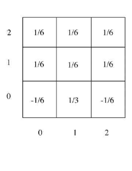
Figure 2: The Wigner function for $p=3$ for the pure state $|\psi\rangle=\frac{1}{\sqrt{2}}(|1\rangle+|2\rangle)$.

V.3 Properties of the Discrete Wigner Function

We now examine whether the definition (25) or, equivalently, (26) satisfies the criteria that we set out in part 1.

1. The mapping is $\rho\rightarrow W_{\rho}$ is linear on $M_{d}$ and convex linear on the density matrices.

2. $W(v)$ is normalized since

$$\sum_{v_{0}v_{1}=0}^{p-1}W(v)=\frac{1}{p^{2}}\left(p^{2}+\sum_{a=0}^{p}\sum_{m=1}^{p-1}\chi(mu_{a})p^{2}\delta(m,0)\right)=1.$$

3. The reality of $W$ follows immediately from Eq. (26).

The first three results also follow directly from Eqs. (27) and (29).

4. For $w\in V_{2}(p)$, if $\rho^{\prime}=S_{w}^{\dagger}\rho S_{w}$ then using Eq. (17)

$$\chi_{\rho^{\prime}}(u) = \eta^{w\circ u}\chi_{\rho}(u)$$

$$W_{\rho^{\prime}}(v) = W_{\rho}(v+w).$$

Note that if $\rho$ commutes with $S_{w}$, the Wigner function is invariant under translations along $w$. Furthermore, the characteristic function vanishes for $u$ such that $w\circ u\neq 0\bmod p$.

5. The marginal distributions are easily computed. We consider the more general case of summing along the points on any of the lines in phase space, where a line in phase space $V_{2}(p)$ is defined as the set of points that satisfy the equation

$$L(b,s) = \{(x,y):-xb+y-s=(x,y)\circ u_{b}-s=0,\quad b,s\in Z_{p}\}$$

$$L(p,s) = \{(s,y):-x+s=(x,y)\circ u_{p}+s=0,\quad b,s\in Z_{p}\}.$$ (31)

$L(b,s)$ is the line with “slope” $b$ which intersects the vertical axis at $s,$ and $L(p,s)$ is a “vertical” line that intersects the horizontal axis at $x=s$ (see Appendix X.5). Let

$$f_{b}(s)=\sum_{v}W(v)\delta(v\circ u_{b}-s,0),$$

then using Eqs. (26) and (21), we can show that

$$f_{b}(s) = \frac{1}{p}\left(-p+\sum_{a\neq b}tr\left[\rho\sum_{r=0}^{p-1}P_{u_{a}}(r)\right]+p\ tr\left[\rho P_{u_{b}}(s)\right]\right)$$

$$= tr\left[\rho P_{u_{b}}(s)\right].$$

We have used the fact that for $a\neq b$ the sum over $v$ becomes a sum over $Z_{p}$, and this sum is the identity operator, while for $a=b$, we have $v\circ u_{b}=s.$ Therefore, we see that summing the Wigner function over any line in phase space gives the probablilty that the system is in the corresponding MUB state.

6. Since $W_{\rho}$ and $\chi_{\rho}$ are Fourier transforms of one another, Plancheral’s formula gives

$$p^{2}\sum_{v}W_{\rho}(v)^{2}=|\chi_{\rho}(0)|^{2}+\sum_{a=0}^{p}\sum_{m=1}^{p-1}|\chi_{\rho}(mu_{a})|^{2}.$$ (32)

We also have, setting $mu_{a}=(j,k)=v,$

$$|\chi_{\rho}(v)|^{2}=|tr\rho S_{v}|^{2}=\langle\rho,S_{v}\rangle\langle S_{v},\rho\rangle.$$

using Eq. (7). More generally,

$$\chi_{\rho_{1}}^{*}(v)\chi_{\rho_{2}}(v)=\left(tr\rho_{1}S_{v}\right)^{*}tr\rho_{2}S_{v}=\langle\rho_{1},S_{v}\rangle\langle S_{v},\rho_{2}\rangle.$$

Summing over the complete set of $S_{v}$, from Eq. (14), we can write Plancheral’s formula,

$$tr\left[\rho_{1}\rho_{2}\right]=p\sum_{v}W_{\rho_{1}}(v)W_{\rho_{2}}(v).$$ (33)

See also Woottersphase where the derivation is based on Eq. (28).

The support of a function $f(v)$ on phase space is defined by

$$supp(f)=\{v\in V_{2}(p):\text{ }f(v)\neq 0\}$$ (34)

and $|supp(f)|$ is defined as the number of points in $supp(f).$ From Eq. (33) we have

$$pW_{\rho}^{2}(v_{0})\leq p\sum_{v}W_{\rho}^{2}(v)=tr\rho^{2}\leq 1.$$ (35)

which implies that for any point $v_{0},$

$$|W(v_{0})|\leq\frac{1}{\sqrt{p}}.$$

Now let

$$\mu_{W_{\rho}}(v)=\left\{\begin{array}[]{ll}1&v\in suppW_{\rho}\\ 0&\text{otherwise.}\end{array}\right.$$

Then applying the Schwarz inequality to the normalization equation and using Eq. (35) we get

$$1=\sum_{v}W_{\rho}(v)\mu_{W_{\rho}}(v)\leq\sqrt{\sum_{v}W_{\rho}^{{2}}(v)\mu_{W_{\rho}}(v)\sum_{u}\mu_{W_{\rho}}(u)}\leq\sqrt{\frac{1}{p}|suppW_{\rho}|}$$

or

$$|suppW_{\rho}|\geq p.$$

This is analogous to the continuous case where the uncertainty principle implies that $W(q,p)$ can not be concentrated into too small a region. We have seen that if $\rho$ is a pure state selected from the MUB that $|suppW_{\rho}|=p,$ and $W_{\rho}(v)=1/p$ on its support, so the lower bound is attained.

If $\rho_{1}$ and $\rho_{2}$ correspond to orthogonal states, then Eq. (33) gives

$$\sum_{v}W_{\rho_{1}}(v)W_{\rho_{2}}(v)=0,$$

which along with the normalization condition implies that, either $suppW_{\rho_{1}}$ and $suppW_{\rho_{2}}$ are disjoint or at least one of the Wigner functions must take on negative values. For example, we saw in V.2.2 that the orthogonal states in one of the bases of a set of MUB have support on non-intersecting lines of $V_{2}(p)$.

There is an inequality, referred to as an uncertainty principle, that also follows from the discrete Fourier transform:

$$|suppW_{\rho}|\text{ }|supp\chi_{\rho}|\geq p^{2},$$

Terras . Equality holds for the random state discussed in example V.2.3 above.

V.4 Inversion formula

In the case of continuous phase space, the density matrix for a particle confined to one-dimension can be obtained from Eq. (6) by using the inverse Fourier integral. We can proceed in a similiar manner for the discrete case. First using the discrete Fourier inversion formula,

$$\chi\left(mu_{a}\right)=\sum_{v\in V(p^{2})}W(v)\eta^{-v\circ mu_{a}}$$ (36)

Then from Eq. (22) and the completeness of the spin matrices

$$\rho=\frac{1}{p}\left(S_{0,0}+\sum_{a=0}^{p}\sum_{m=1}^{p-1}\chi\left(mu_{a}\right)^{*}S_{u_{a}}^{m}\right).$$ (37)

Substituting (36) into (37), and using Eqs. (15) and (27), we also get

$$\rho=\sum_{v\in V(p^{2})}W(v)A(v).$$ (38)

Therefore, we have an expression for the density matrix as an expansion in the spin matrices with coefficients given by the characteristic function and an equivalent expansion in terms of a basis of Hermitian operators with the Wigner function as coefficients.

VI Mutually Unbiased Bases II

To define the generalized spin matrices in the case when $d=p^{n}$ where $p$ is prime, we require the notion of a finite or Galois field $GF(p^{n}),$ see Appendices X.1 and X.2 for more details. There is a systematic way of representing the elements in $GF\left(p^{n}\right)$ that uses the structure of polynomials irreducible over $GF\left(p\right)=Z_{p}.$ An irreducible polynomial is a polynomial $f(x)$ of degree $n$ with coefficients in $GF(p)$ that can not be factored into non-constant polynomials of lower degree. Then the elements of $GF(p^{n})$ may be represented by polynomials of degree less than $n$ with coefficients in $GF(p)$. The simplest example is that of two qubits, $p=2,$ $n=2$. In this case the irreducible polynomial is unique and is given by $x^{2}+x+1$. Define $\lambda$ to be a symbolic solution of $x^{2}+x+1=0$ $\bmod{2}.$ Then every element of $GF(2^{2})$ can be written as $\alpha=a_{0}+\lambda a_{1}$ where $a_{0}$ and $a_{1}$ are in $GF(2)$ . This is analogous when working with real numbers to letting $i$ denote a symbolic solution of the equation $x^{2}+1=0$ and introducing complex numbers as $x+iy.$

For the case of $n=2$ and $p$ an odd prime, let $D$ be an element in $GF\left(p^{2}\right)$ such that there is no solution in $Z_{p}=GF(p)$ to the equation $x^{2}-D=0$ $\bmod{p}$. In technical terms, $D$ is a quadratic non-residue of $p$. There are an equal number of quadratic residues and quadratic non-residues in $GF(p)$. Then elements in $GF\left(p^{2}\right)$ can be represented as $j+k\lambda$, where $j$ and $k$ are in $GF\left(p\right)$ and $\lambda$ is taken to be a symbolic solution of $x^{2}-D=0$ $\bmod{p}$ . Addition and multiplication of elements of $GF(p^{2})$ are defined by

$$(j_{1}+k_{1}\lambda)+(j_{2}+k_{2}\lambda) = (j_{1}+j_{2})+(k_{1}+k_{2})\lambda$$

$$(j_{1}+k_{1}\lambda)(j_{2}+k_{2}\lambda) = (j_{1}j_{2}+Dk_{1}k_{2})+(j_{1}k_{2}+k_{1}j_{2})\lambda,$$

where the additions in the parentheses are modulo $p$. We refer to Appendix X.2 for more details.

We can construct a complete set of mutually unbiased bases when $d=p^{n}$ by following the same procedure that was used in the $d=p$ case Wootters0 . The key idea for constructing a MUB is based on the fact that we can define a two-dimensional vector space $V_{2}(p^{n})$ over $GF(p^{n})$, and $p^{n}+1$ generating vectors $u_{\alpha}$ where $\alpha$ is in the index set $I_{p^{n}}=GF(p^{n})\cup\{p^{n}\}.$ Specifically, define

$$u_{\alpha}=\left\{\begin{array}[]{ll}(1,\alpha),&\alpha\in GF(p^{n})\\ (0,1),&\alpha=p^{n}\end{array}\right.$$ (39)

Each of these vectors can be used to define a class containing $p^{n}$ vectors,

$$C_{\alpha}=\{\beta u_{\alpha},\beta\in GF(p^{n})\}$$ (40)

where $\alpha\in I_{p^{n}}.$ Each pair of vectors in a class has vanishing symplectic product, Eq. (11) where the operations are with respect to $GF(p^{n})$. We want to find a spin matrix representation of these classes, that is, we wish to find a mapping from this space to the set of tensor products

$$S_{\mathbf{u}}=\bigotimes_{r=0}^{n-1}S_{u_{r}}$$ (41)

where $\mathbf{u}=\bigoplus\limits_{r=0}^{n-1}u^{(r)}$ $\in V_{2n}(p)$ and each $u^{(r)}\in V_{2}^{(r)}(p)=V_{2}(p).$ To do this we define an isomorphism

$$M:V_{2}(p^{n})\rightarrow V_{2n}(p)=\bigoplus_{j=0}^{n-1}V_{2}^{(j)}(p)$$

that preserves the symplectic product in the following sense. For each vector $v\in V_{2}(p^{n}),$ if $M(v)=\mathbf{v}=\bigoplus_{j=0}^{n-1}u^{(j)},$ where $u^{(j)}\epsilon V_{2}^{(j)}(p),$ define

$$\mathbf{v}_{1}\circ\mathbf{v}_{2}=\sum_{j=0}^{p-1}(u_{1}^{(j)}\circ u_{2}^{(j)}).$$ (42)

Then $v_{1}\circ v_{2}=0$ implies $\mathbf{v}_{1}\circ\mathbf{v}_{2}=0$ as is shown in Eq. (87). We present an outline of the derivation of $M$ in Appendix X.2 and refer to PRMUB for another discussion. It is worth noting that the construction of $V_{2n}(p)$ is analogous to what is done in the continuous case. There we take the direct sum of the two-dimensional vector spaces corresponding to independent conjugate position and momentum pairs.

To perform the analog of what was done in Eq. (18), it is useful to introduce the generators of the index set for the set of MUB, again the details are given in Appendix X.2. For $\alpha\in I_{p^{n}},$ define $\lambda^{r}u_{\alpha}\in V_{2}(p^{n}),\ r=0,\cdots,n-1.$ Then define a set of generators on $V_{2n}(p)$

$$G_{\alpha}=\{\mathbf{g}_{r}(\alpha)=M\left(\lambda^{r}u_{\alpha}\right),\text{ }r=0,\cdots,n-1\},$$ (43)

and define the corresponding spin matrix using Eq. (41) as

$$S_{\mathbf{g}_{r}(\alpha)}^{b}\equiv\bigotimes_{j=0}^{n-1}S_{u_{r}^{(j)}(\alpha)}^{b}$$ (44)

where each $S_{u^{(j)}}$ acts on a Hilbert space $H_{p}.$ The generalization of Eq. (18) is

$$G_{\alpha}\rightarrow\mathfrak{M}_{\alpha}=\left\{\prod\limits_{r=0}^{n-1}S_{\mathbf{g}_{r}(\alpha)}^{b_{r}}=\bigotimes\limits_{j=0}^{n-1}\prod\limits_{r=0}^{n-1}S_{u_{r}^{(j)}(\alpha)}^{b_{r}},\quad b_{r}\in GF(p)\right\}$$ (45)

for the generation of $p^{n}+1$ disjoint sets of $p^{n}$ of commuting operators $\mathfrak{M}_{\alpha}$ where $\mathfrak{M}_{\alpha}\cap\mathfrak{M}_{\beta}=\{S_{0,0}\}$ for all $\alpha\neq\beta.$ We have written the mapping in Eq. (45) from the set of basis vectors $G_{\alpha}$ rather than the space $C_{\alpha}$.

It is also possible to write down the set $\left\{P_{\alpha}\left(r\right),r\in V_{n}\left(p\right)\right\}$ of rank one orthogonal projections defined by each of the $p^{n}+1$ commuting classes $\mathfrak{M}_{\alpha}.$ This gives the set of MUB as projections defined explicitly in terms of sums of the spin matrices in each class. The procedure to do this is discussed in PRMUB , and is illustrated there for the case for $n=2$ . The corresponding projection operators for the case $p>2$ are

$$P_{\alpha}(\mathbf{s}) = \prod_{r=0}^{n-1}P_{\mathbf{g}_{r}(\alpha)}(s_{r})$$

$$P_{\mathbf{g}_{r}(\alpha)}(s_{r}) = \left(\frac{1}{p}\sum_{b_{r}=0}^{p-1}\left[\eta^{s_{r}}S_{\mathbf{g}_{r}(\alpha)}\right]^{b_{r}}\right),$$ (46)

where $\mathbf{s}=(s_{0},\ldots,s_{n-1}).$ For $p=2$ it is necessary to include the factors $\alpha_{2}(j,k)$ in the definition of the projection operators as shown in Eq. (15). $P_{\alpha}\left(\mathbf{r}\right)$ has trace one, and it is straightforward to check that if $\mathbf{r}\neq\mathbf{s}$

$$P_{\alpha}(\mathbf{r})P_{\alpha}(\mathbf{s})=\delta(\mathbf{r},\mathbf{s})P_{\alpha}(\mathbf{r}).$$

It is easy to show that each $P_{\alpha}\left(\mathbf{r}\right)$ is a product of commuting projections. One can also show that $P_{\alpha}\left(\mathbf{r}\right)=\left(P_{\alpha}\left(\mathbf{r}\right)\right)^{\dagger}$, and it follows that $P_{\alpha}\left(\mathbf{r}\right)$ is a rank one orthogonal projection and that

$$I=\sum_{\mathbf{r}}P_{\alpha}\left(\mathbf{r}\right).$$

Finally, it can be shown that for $\alpha\neq\beta$ that

$$tr\left[P_{\alpha}(\mathbf{r})P_{\beta}(\mathbf{s})\right]=\frac{1}{1/p^{n}}.$$

The explicit calculation of the projections and of the set of vectors in $V_{2n}\left(p\right)$ corresponding to $C_{\alpha}$ depends quite specifically on $p$ and $n$ and on the representation of elements in the different finite fields. When $n=2$ and $p$ is an odd prime, however, one can give a unified summary of the results of the theory. Without going through the detailed construction outlined in Appendix X.2, it is easy to check that the vectors in each of the classes below have symplectic product zero.

Example d=p²

Let $d=p^{2}$ with $p$ an odd prime and $D$ such that $x^{2}-D=0$ $\bmod{p}$ has no solution in $GF(p).$ In Appendix X.2, Eq. (92) it is shown that the $p^{2}+1$ commuting classes of indices are generated by

$$G_{a_{0},a_{1}}=\left\{\left(1,2a_{0},0,2Da_{1}\right),\left(0,2Da_{1},1,2Da_{0})\right)\right\}$$

where $a_{0}$ and $a_{1}$ are in $GF(p)$, and

$$G_{p^{2}}=\left\{\left(0,1,0,0\right),\left(0,0,0,1)\right)\right\}.$$

One can check directly that the vectors in each $G_{a_{0},a_{1}}$ have vanishing symplectic product. Then the spin matrices that generate the commuting classes may be written as

$$G_{a_{0},a_{1}} \rightarrow \mathfrak{M}_{(a_{0},a_{1})}=\left\{\left(S_{1,2a_{0}}\otimes S_{0,2Da_{1}}\right)^{b_{0}}\left(S_{0,2Da_{1}}\otimes S_{1,2Da_{0}}\right)^{b_{1}},\text{ }b_{0},b_{1}\in GF(p)\right\},$$

$$G_{p^{2}} \rightarrow \mathfrak{M}_{p^{2}}=\left\{\left(S_{0,1}^{b_{0}}\otimes S_{0,0}\right)\left(S_{0,0}\otimes S_{0,1}^{b_{1}}\right),\ b_{0},b_{1}\in GF(p)\right\}.$$ (47)

The corresponding projections are given by

$$P_{a_{0},a_{1}}\left(\left(r_{0},r_{1}\right)\right) = \frac{1}{p}\sum_{b_{0}=0}^{p-1}\left(\left(\eta^{r_{0}}S_{1,2a_{0}}\otimes S_{0,2Da_{1}}\right)^{b_{0}}\right)\frac{1}{p}\sum_{b_{1}=0}^{p-1}\left(\left(\eta^{r_{1}}S_{0,2Da_{1}}\otimes S_{1,2Da_{0}}\right)^{b_{1}}\right)$$

$$P_{p^{2}}\left(\left(r_{0},r_{1}\right)\right) = \frac{1}{p}\sum_{b_{0}=0}^{p-1}\left(\left(\eta^{r_{0}}S_{0,1}\otimes S_{0,0}\right)^{b_{0}}\right)\frac{1}{p}\sum_{b_{1}=0}^{p-1}\left(\left(\eta^{r_{1}}S_{0,0}\otimes S_{0,1}\right)^{b_{1}}\right).$$

We note that each of these one-dimensional projection operators is the product of two commuting rank $p$-dimenional projections. The two $p$ -dimensional spaces that they project onto intersect in a one-dimensional space.

VII Wigner Function For $d=p^{2}$

In earlier work Woottersphase ; Paz , the phase space on which the Wigner functions were defined when $d=p^{n}$ was chosen to be $V_{2}(p^{n})$. The advantage of this choice is that one can use the underlying geometry to great advantage. The disadvantage is that one has to label coordinates using elements from the Galois field $GF(p^{n})$ which does not lend itself to a discussion of separability. However, as we saw in Section VI, and as is elaborated in Appendix X.2, there is a natural isomorphism M between $V_{2}(p^{n})$ and $V_{2n}(p)$ which encodes the geometry of $V_{2}(p^{n})$ in $V_{2n}(p)$. We take advantage of this structure to define our Wigner function on $V_{2n}(p)$ This is in close analogy to the continuous case and simplifies computations involving the generalized spin matrices.

In particular, this approach enables questions involving separability to be treated efficiently. In this section we illustrate the ideas in detail for $n=2$, leaving the generalizations to the next section and the Appendix.

VII.1 Separability of the Wigner Function for $p$ an odd prime

We consider a bipartite system composed of subsystems of dimension $p,$ a prime. As we saw in Section 5, there is a certain latitude in the definition of the Wigner function that is available because of the freedom to include phase factors in the characteristic function. Our goal in this section is to show how that freedom enables us to define Wigner functions for one and two subsystems so that separability is respected. Specifically, for a product state we want

$$\rho=\tau\otimes\mu\Rightarrow W_{\rho}\left(\mathbf{u}\right)=W_{\tau}\left(u^{(0)}\right)W_{\mu}\left(u^{(1)}\right),$$ (48)

where $\mathbf{u}=u^{(0)}\oplus u^{(1)}.$ Then, since $W_{\rho}\left(\mathbf{u}\right)$ is convex linear on the space of densities, we will have the general statement that

$$\rho=\sum_{k}p_{k}\tau_{k}\otimes\mu_{k}\Rightarrow W_{\rho}\left(\mathbf{u}\right)=\sum_{k}p_{k}W_{\tau_{k}}\left(u^{(0)}\right)W_{\mu_{k}}\left(u^{(1)}\right).$$ (49)

A natural definition of the characteristic function $\chi=\chi_{\rho}$ is to use Eq. (44) with $n=2,$ and define

$$\widetilde{\chi}(\mathbf{w})=tr\left[\rho S_{\mathbf{g}_{0}(\alpha)}^{b_{0}}S_{\mathbf{g}_{1}(\alpha)}^{b_{1}}\right]$$ (50)

where $\mathbf{w}=b_{0}\mathbf{g}_{0}(\alpha)+b_{1}\mathbf{g}_{1}(\alpha).$ We can rewrite the product of the $S$ matrices on $H_{p^{2}}$ as a direct product of $S$ matrices on $H_{p}^{(0)}\otimes H_{p}^{(1)}.$ Rewriting $\mathbf{w}=u^{(0)}\oplus u^{(1)}$ where $u^{(j)}\in V_{2}^{(j)}(p),$ we find

$$\widetilde{\chi}(\mathbf{w})=\eta^{\Phi}tr\left[\rho S_{u^{(0)}}\otimes S_{u^{(1)}}\right].$$

The problem with this definition is that in general $\Phi\neq\phi(u^{(0)})+\phi(u^{(1)}),$ so that the corresponding Wigner function would not factor when $\rho$ is a product state. Now as pointed out before, there is some freedom in the choice of phase in defining the characteristic function and the Wigner function. For this reason it is convenient to introduce a phase factor into the definition of the characteristic function to avoid this problem. We shall therefore define the characteristic function as

$$\chi(\mathbf{w})=\eta^{-\Theta}\widetilde{\chi}(\mathbf{w)},$$ (51)

using Eq. (50) and the $\Theta$ defined in Eq. (99) that is linear in $b_{0}$ and $b_{1}$. The linearity in the $b^{\prime}s$ is important, as we shall see, because we want to write the analog of Eq. (26) with the appropriate projection operators given in Eq. (46).

The underlying reason for having to introduce the phases arises from the fact that we are using the geometries of $V_{2}(p^{2})$ and $V_{4}(p)$. That fact forces us to go into some detail to define appropriate phase factors and to confirm that they work.

For example, consider the case of $p$ odd discussed at the end of the last section. For $\alpha\neq p^{2}$ define

$$\chi_{\rho}\left(\mathbf{w}\right)=Tr\left[\rho\left(\eta^{-Da_{1}}S_{\mathbf{g}_{0}}\right)^{b_{0}}\left(\eta^{-Da_{1}}S_{\mathbf{g}_{1}}\right)^{b_{1}}\right],$$ (52)

and for $\alpha=p^{2}$ define

$$\chi_{\rho}\left(\mathbf{w}\right)=Tr\left[\rho\left(\eta^{-2^{-1}}S_{\mathbf{g}_{0}}\right)^{b_{0}}\left(\eta^{-2^{-1}}S_{\mathbf{g}_{1}}\right)^{b_{1}}\right].$$ (53)

Then define

$$W_{\rho}\left(\mathbf{u}\right)=\frac{1}{p^{4}}\sum_{\mathbf{w}}\eta^{\mathbf{u}\circ\mathbf{w}}\chi_{\rho}\left(\mathbf{w}\right).$$ (54)

Note again that $-2^{-1}$ is computed modulo $p$ and equals $\left(p-1\right)/2.$ The vector symplectic product in the exponent of $\eta$ is defined in Eq. (42). From Eq. (25) we can write out the right hand side of Eq. (48) with one modification. For $mu_{p}=m\left(0,1\right)$ take

$$\chi_{\tau}(mu_{p})=tr\left[\tau\left(\eta^{-2^{-1}}S_{u_{p}}\right)^{m}\right],$$ (55)

as we did in Example 4 of Section V. Then $W_{\tau}\left(u\right)$ is defined as the usual symplectic tranform and can be written as

$$W_{\tau}\left(u\right)=\frac{1}{p^{2}}\left[\sum_{m=0}^{p-1}\eta^{u\circ mu_{p}}\chi_{\tau}\left(mu_{p}\right)+\sum_{c=0}^{p-1}\sum_{m=1}^{p-1}\eta^{u\circ mu_{c}}\chi_{\tau}\left(mu_{c}\right)\right].$$ (56)

Finally, we get the right hand side of Eq. (48) as the trace of $\frac{1}{p^{2}}\left(\tau\otimes\mu\right)$ times the expression

$$rhs = \sum_{m_{0}=0}^{p-1}\sum_{m_{1}=0}^{p-1}\eta^{\mathbf{u}\circ\left(0,m_{0},0,m_{1}\right)}\eta^{-2^{-1}\left(m_{0}+m_{1}\right)}S_{m_{0}u_{p}}\otimes S_{m_{1}u_{p}}+$$

$$\sum_{\left(c_{0},c_{1}\right)\neq\left(p,p\right)}\sum_{\left(m_{0},m_{1}\right)\neq\left(0,0\right)}\eta^{\mathbf{u}\circ\left(m_{0}u_{c_{0}}\oplus m_{1}u_{c_{1}}\right)}\eta^{-2^{-1}\left(\delta\left(c_{0},p\right)m_{0}+\delta\left(c_{1},p\right)m_{1}\right)}\left(S_{u_{c_{0}}}\right)^{m_{0}}\otimes\left(S_{u_{c_{1}}}\right)^{m_{1}}.$$

The left hand side of Eq. (48) can be written as the trace of $\frac{1}{p^{2}}\left(\tau\otimes\mu\right)$ times the expression

$$lhs = \sum_{b_{0}=0}^{p-1}\sum_{b_{1}=0}^{p-1}\eta^{\mathbf{u}\circ\left(b_{0}\mathbf{g}_{0}\left(p^{2}\right)+b_{1}\mathbf{g}_{1}\left(p^{2}\right)\right)}\eta^{-2^{-1}\left(b_{0}+b_{1}\right)}S_{\left(0,b_{0},0,b_{1}\right)}+$$

$$\sum_{\alpha\neq p^{2}}\sum_{\left(b_{0},b_{1}\right)\neq\left(0,0\right)}\eta^{\mathbf{u}\circ\left(b_{0}\mathbf{g}_{0}\left(\alpha\right)+b_{1}\mathbf{g}_{1}\left(\alpha\right)\right)}\eta^{-Da_{1}\left(b_{0}+b_{1}\right)}\left(S_{\mathbf{g}_{0}(\alpha)}\right)^{b_{0}}\left(S_{\mathbf{g}_{1}(\alpha)}\right)^{b_{1}}.$$

Note that in this equation we have the ordinary matrix product in the second term.

Our goal is to confirm that Eq. (48) holds with the above definitions of the characteristic functions. Using Eq. (12) we can pair the indices of the spin matrices in Eq. (48) to obtain the index equation relating terms in rhs to lhs,

$$\mathbf{w}=m_{0}u_{c_{0}}\oplus m_{1}u_{c_{1}}=b_{0}\mathbf{g}_{0}\left(\alpha\right)+b_{1}\mathbf{g}_{1}\left(\alpha\right),$$ (57)

which includes the $\mathbf{w}=\left(0,0,0,0\right)$ term that is incorporated in the first summations. It follows that the phase factor $\eta^{\mathbf{u}\circ\left(b_{0}\mathbf{g}_{0}\left(\alpha\right)+b_{1}\mathbf{g}_{1}\left(\alpha\right)\right)}$ is common to the corresponding terms of $rhs$ and $lhs$, and we can cancel it. It is also obvious that the $\alpha=p^{2}$ terms equal the corresponding terms associated with $c_{0}=c_{1}=p$ and that the remaining phase factors in this case are also equal if we set $m_{k}=b_{k}$.

To match terms in the second sets of summations, we multiply out the powers of the spin matrices in lhs to obtain

$$S_{m_{0}u_{c_{0}}}\otimes S_{m_{1}u_{c_{1}}}=S_{b_{0}\left(1,2a_{0}\right)+b_{1}\left(0,2Da_{1}\right)}\otimes S_{b_{0}\left(0,2Da_{1}\right)+b_{1}\left(1,2Da_{0}\right)},$$

where the equality follows from the index equation. This process introduces phase factors using Eqs.(10) and (12), and it remains to prove that the resulting exponents of $\eta$ are equal. Specifically, one has to verify that subject to Eq. (57)

$$\left(1-\delta\left(c_{0},p\right)\right)c_{0}\binom{m_{0}}{2}+\left(1-\delta\left(c_{1},p\right)\right)c_{1}\binom{m_{1}}{2}-2^{-1}\left(\delta\left(c_{0},p\right)m_{0}+\delta\left(c_{1},p\right)m_{1}\right)$$ (58)

equals

$$-Da_{1}\left(b_{0}+b_{1}\right)+2a_{0}\binom{b_{0}}{2}+2Da_{0}\binom{b_{1}}{2}+2b_{0}b_{1}Da_{1}.$$ (59)

We verify the equality for $\alpha\neq p^{2}$ by considering different cases. Let $\alpha=a_{0}+a_{1}\lambda$. If $b_{0}$ and $b_{1}$ are both non-zero, $m_{0}=b_{0},$ $m_{1}=b_{1}$ and

$$b_{0}c_{0} = b_{0}2a_{0}+b_{1}2Da_{1},$$

$$b_{1}c_{1} = \left(b_{0}2Da_{1}+b_{1}2Da_{0}\right).$$

If $b_{0}=0,$

$$\mathbf{w}=(0,b_{1}2Da_{1})\oplus(b_{1},b_{1}2Da_{0})$$

and $c_{0}=p,$ $m_{0}=b_{1}2Da_{1},$ $c_{1}=2Da_{0}$ and $m_{1}=b_{1}.$ Similarly, for $b_{1}=0$

$$\mathbf{w}=(b_{0},b_{0}2a_{0})\oplus(0,b_{0}2Da_{1}),$$

and $m_{0}=2Da_{0},$ $m_{0}=b_{0},$ $m_{0}=p$ and $m_{1}=b_{0}2Da_{1}.$ Substituting these expressions in Eq. (58) gives (59). We have gone through this in some detail because the method illustrated generalizes to the case of complete separability of $n$ subsystems. It should be noted that the argument leading to Eq. (48) did not require that $\tau$ or $\mu$ be a density matrix.

Our ability to add a phase factor to the definition of the characteristic function is related to an arbitrariness in the assigning of state vectors in a basis on the Hilbert space to lines in phase space as noted in Woottersphase . This is illustrated in VII.3.2 below.

A different definition of the Wigner function in terms of the characteristic function can be found in Vourdas . Vourdas replaces the $M$ transformation by introducing the trace operation into the Fourier transformation.

VII.2  Properties of the Wigner Function

Because we have used the same format in defining the Wigner function for two subsystems, Eq. (54), as was used in defining it for a single subsystem, Eq. (25), we expect the properties in Section II to hold. With the definition of $\chi_{\rho}(\mathbf{w)}$ in Eqs. (52) and (53) conditions (23) and (24) are satisfied. The discrete Wigner function $W_{\rho}$ for a density $\rho$ on $H_{p^{2}}$ is defined using the symplectic Fourier transform Eq. (54); consequently, $W_{\rho}$ is convex linear on the space of densities and linear on the space of $p^{2}\times p^{2}$ matrices. Again, the defining Eq. (54) is invertible, so that one can obtain the $\chi_{\rho}\left(\mathbf{w}\right)$ and thus the spin coefficients of $\rho$ from the Wigner function. With this definition Plancheral’s formula becomes

$$p^{4}\sum_{\mathbf{v}\in V_{4}(p)}|W(\mathbf{v})|^{2}=|\chi(0)|^{2}+\sum_{q,r=0}^{p}\sum_{M}|\chi(m^{(0)}u_{q}^{(0)}\oplus m^{(1)}u_{r}^{(1)})|^{2}.$$

We also have, as in Eq. (33), that

$$tr\left[\rho_{1}\rho_{2}\right]=p^{2}\sum_{\mathbf{v}}W_{\rho_{1}}(\mathbf{v})W_{\rho_{2}}(\mathbf{v}),$$

and, consequently, $|W(\mathbf{v})|\leq 1/p$ and $|suppW(\mathbf{v})|\geq 1/p^{2}$. Using the notation of Eq. (46), we can write

$$W_{\rho}\left(\mathbf{u}\right)=tr\left[\rho A\left(\mathbf{u}\right)\right]$$ (60)

where

$$p^{2}A\left(\mathbf{u}\right) = -S_{0,0}\otimes S_{0,0}+P_{p^{2}}\left(-2^{-1}+\mathbf{u}\circ\mathbf{g}_{0}\left(p^{2}\right),-2^{-1}+\mathbf{u}\circ\mathbf{g}_{1}\left(p^{2}\right)\right)$$

$$+\sum_{\alpha\neq p^{2}}P_{\alpha}\left(-Da_{1}+\mathbf{u}\circ\mathbf{g}_{0}\left(\alpha\right),-Da_{1}+\mathbf{u}\circ\mathbf{g}_{1}\left(\alpha\right)\right),$$

corresponding to Eq. (27). From Eq. (VII.2) it follows that $W_{\rho}$ is real for densities $\rho$. In particular, $\left\{A(\mathbf{u})\right\}$ again defines a complete orthogonal set of Hermitian matrices. The argument is analogous to that leading to Eq. (27) and leads to

$$Tr\left[A\left(\mathbf{u}\right)A\left(\mathbf{v}\right)\right]=p^{-2}\delta\left(\mathbf{u},\mathbf{v}\right)$$

Thus we can interpret the Wigner function $W_{\rho}$ as the set of coefficients of $\rho$ in the orthogonal expansion relative to $\left\{A(\mathbf{u})\right\}$ analogous to Eq. (38) .

The analogues of the other properties of Section V.3 follow in the same way as before. $W$ is normalized since we can use Eq. (60) to prove

$$\sum_{\mathbf{u}}W_{\rho}\left(\mathbf{u}\right)=Tr\left[\rho\sum_{\mathbf{u}}A\left(\mathbf{u}\right)\right]=Tr\left[\rho\right]=1$$

since Eq. (29) holds in this case. If $\rho^{\prime}=S_{\mathbf{z}}^{\dagger}\rho S_{\mathbf{z}}\in H_{p}\otimes H_{p},$ then $\chi_{\rho^{\prime}}\left(\mathbf{w}\right)=\eta^{\mathbf{z}\circ\mathbf{w}}\chi_{\rho}\left(\mathbf{w}\right)$, and $W_{\rho^{{}^{\prime}}}\left(\mathbf{u}\right)=W_{\rho}\left(\mathbf{u}+\mathbf{z}\right)$ as before.

Summing $W_{\rho}\left(\mathbf{u}\right)$ over a “line” in $V_{2}\left(p^{2}\right)$ corresponds to summing over a translation of a two dimensional subspace in $V_{4}\left(p\right)$ and again leads to a marginal probability $Tr\left[\rho P_{\alpha}\left(s_{1},s_{2}\right)\right]$. To see this let $C_{\alpha}$ denote the two dimensional subspace associated with $\alpha$. It is easy to show that

$$\sum_{\mathbf{u}\in C_{\alpha}}W_{\rho}\left(\mathbf{u}+\mathbf{r}\right)=\frac{1}{p^{2}}\sum_{\mathbf{w}\in C_{\alpha}}\eta^{\mathbf{r}\circ\mathbf{w}}\chi_{\rho}\left(\mathbf{w}\right).$$

This can be written as the trace of $\rho$ against the projection $P_{\alpha}\left(s_{1},s_{2}\right)$ for appropriate indices $s_{1}$ and $s_{2}$ which depend on $\mathbf{r}$ and the phase factors used in the definition of the characteristic functions. Thus using definition of Eq. (54) the Wigner function satisfies the conditions proved in section V.3 and the requirement that $W_{\rho}$ factor for separable $\rho$ as in Eq. (49).

As pointed out to us by Wootters, Eq. (48) may be used to give a positive answer to a question posed in Woottersphase . That is, with the phase factors given above, we have

$$A(\mathbf{u})=A(u^{(0)})\otimes A(u^{(1)}).$$

where $\mathbf{u}=u^{(0)}\oplus u^{(1)}.$ The proof is easy, rewrite Eq. (48) as

$$tr\left[\tau_{0}\otimes\tau_{1}A(\mathbf{u})\right]=tr\left[\tau_{0}\otimes\tau_{1}A(u^{(0)}\oplus A(u^{(1)})\right].$$

This equality holds even the $\tau$’s are not densities. Since Hermitian matrices of the form $\tau\otimes\mu$ form a basis of $M_{p^{2}}$, this inequality holds for all $A(\mathbf{u})$ for all $\mathbf{u}\in V_{4}(p)$.

VII.3 Examples

VII.3.1 Maximally entangled state

For prime $p$ let $\left|\Psi\right\rangle=\frac{1}{\sqrt{p}}\sum_{j}\left|j\right\rangle\left|j\right\rangle$, so that $\rho\equiv\left|\Psi\right\rangle\left\langle\Psi\right|=\frac{1}{p}\sum_{j,k}$ $\left|j\right\rangle\left\langle k\right|\otimes\left|j\right\rangle\left\langle k\right|$. By the separability property and linearity we know that if $\mathbf{u}=u^{(0)}\oplus u^{(1)}=\left(x_{0},y_{0},x_{1},y_{1}\right)$, then

$$W_{\rho}\left(\mathbf{u}\right)=\frac{1}{p}\sum_{j,k}W_{\left|j\right\rangle\left\langle k\right|}\left(u^{(0)}\right)W_{\left|j\right\rangle\left\langle k\right|}\left(u^{(1)}\right),$$

where $W_{\left|j\right\rangle\left\langle k\right|}\left(u\right)$ is defined in Eq. (30). It follows that

$$W_{\rho}\left(\mathbf{u}\right)=\frac{1}{p^{3}}\sum_{j,k}\eta^{\left(x_{0}+x_{1}+1\right)\left(k-j\right)}\delta\left(y_{0}+2^{-1}(j+k),0\right)\delta\left(y_{0}+2^{-1}\left(j+k\right),0\right),$$

and simplifying we get

$$W_{\rho}\left(\mathbf{u}\right)=\frac{1}{p^{2}}\delta\left(1+x_{0}+x_{1},0\right)\delta\left(y_{0},y_{1}\right)$$

Thus the Wigner function for this maximally entangled state equals $1/p^{2}$ for the $p^{2}$ four-vectors with $u^{(0)}=(x_{0},y_{0})$ and $u^{(1)}=\left(-1-x_{0},y_{0}\right)$ and equals zero elsewhere.

Although the Wigner function for this state is positive, it is a non-classical state. In particular, entangled states violate Bell inequalities. Since the Wigner function discussed in this example is not separable, it need not respect mathematical inequalities based on separability.

VII.3.2 MUB

Let $\rho=P_{\alpha}\left(s_{0},s_{1}\right).$ In this case it is simplest to use Eq. (VII.2) so that

$$W_{\rho}(\mathbf{u}) = \frac{1}{p^{2}}tr\left[P_{\alpha}\left(s_{0},s_{1}\right)A(\mathbf{u})\right]$$

$$= \frac{1}{p^{2}}\left[-1+\sum_{\beta\neq\alpha}Tr\left[P_{\alpha}\left(s_{0},s_{1}\right)P_{\beta}\left(r_{0,\beta}\left(\mathbf{u}\right),r_{1,\beta}\left(\mathbf{u}\right)\right)\right]+Tr\left[P_{\alpha}\left(s_{0},s_{1}\right)P_{\alpha}\left(r_{0,\alpha}\left(\mathbf{u}\right),r_{1,\alpha}\left(\mathbf{u}\right)\right)\right]\right]$$

$$= \frac{1}{p^{2}}\left[-1+p^{2}/p^{2}+\delta\left(s_{0},r_{0,\alpha}\left(\mathbf{u}\right)\right)\delta\left(s_{1},r_{1,\alpha}\left(\mathbf{u}\right)\right)\right]$$

$$= \frac{1}{p^{2}}\delta\left(s_{0},r_{0,\alpha}\left(\mathbf{u}\right)\right)\delta\left(s_{1},r_{1,\alpha}\left(\mathbf{u}\right)\right)$$

Thus, $W_{\rho}\left(\mathbf{u}\right)$ equals $1/p^{2}$ on those $p^{2}$ four-vectors which match the given phases and equals zero elsewhere. For $\alpha\neq p^{2},$ $r_{k,\alpha}\left(\mathbf{u}\right)=-Da_{1}+\mathbf{u}\circ\mathbf{g}_{k}\left(\alpha\right),$ and it can be shown easily that the set of four-vectors satisfying those conditions is

$$\left\{\mathbf{u}=b_{0}\mathbf{g}_{0}\left(\alpha\right)+b_{1}\mathbf{g}_{1}\left(\alpha\right)+\left(0,s_{0}+Da_{1},0,s_{1}+Da_{1}\right):b_{0},b_{1}\in GF(p)\right\}.$$

That is, $W_{\rho}\left(\mathbf{u}\right)$ is constant on a shift of the two-dimensional subspace indexed by $\alpha.$ An analogous result holds if $\alpha=p^{2}$, and, as expected, this parallels the situation when $n=1.$

VII.4 Separability of the Wigner function for p=2

When $p=2$ Eq. (54) can be used to define the Wigner function with the definition of the characteristic function given in Eq. (62) below. Properties other than separability follow as before, but the analysis leading to separability for $p$ odd does not work in this case. The discussion above made use of the existence of a quadratic non-residue $D$; however, for $p=2$ no such quantity exists. In addition we must include the factors of $\alpha_{2}=\alpha_{2}(1,1)=-i$ defined at the end of III.

Explicit forms of generating vectors are

$$G_{a_{0},a_{1}}=\{(1,a_{1},0,a_{0}+a_{1}),(0,a_{0}+a_{1},1,a_{0})\}$$

for $\alpha=a_{0}+a_{1}\lambda\in GF(2^{2})$, and

$$G_{4}=\{(1,0,0,0),(0,0,1,0)\}.$$

For the case $\alpha\neq 2^{2}$, the analog of Eq. (52) is

$$\chi_{\rho}(\mathbf{w})=Tr[\rho(\alpha_{2}^{a_{1}}\eta^{r_{0}}S_{\mathbf{g}_{0}})^{b_{0}}(\alpha_{2}^{a_{0}}\eta^{r_{1}}S_{\mathbf{g}_{1}})^{b_{1}}]$$ (62)

where $r_{0}$ and $r_{1}$ depend on $a_{0}$ and $a_{1}$. It is convenient to write the index equation Eq. (57) in the form

$$\mathbf{w}=(b_{0},q_{0})\oplus(b_{1},q_{1})=b_{0}\mathbf{g}_{0}(\alpha)+b_{1}\mathbf{g}_{1}(\alpha),$$

then it is not difficult to show that for $(b_{0},b_{1})\neq(0,0)$

$$a_{0} = b_{0}q_{0}+(b_{0}+b_{1})q_{1}$$

$$a_{1} = (b_{0}+b_{1})q_{0}+b_{1}q_{1}.$$

This allows us to replace the sums in the Wigner function over $a_{0}$ and $a_{1}$ by sums over $q_{0}$ and $q_{1}$. Now we can write

$$\chi_{\rho}(\mathbf{w})=\eta^{(b_{0}r_{0}+b_{1}r_{1})}\alpha_{2}^{(b_{0}q_{0}+b_{1}q_{1})}\eta^{b_{0}b_{1}(q_{0}+q_{1})}Tr[\rho S_{b_{0},q_{0}}\otimes S_{b_{1},q_{1}}].$$ (63)

As stated above, we require that the phase factors are linear in the b’s. In order to enforce this it is easy to show that if $r_{0}=0$ and $r_{1}=a_{0}=b_{0}q_{0}+b_{1}(a_{0}+a_{1})$ the exponent of $\eta$ is simply $b_{1}q_{1}$. This calculation makes use of the binary arithmetic, in particular $b^{2}=b$.

Finally, we find that for $\rho=\tau\otimes\mu$ the phase factor $\eta^{b_{1}q_{1}}$ requires that we use different one particle Wigner functions for the two particles. Equivalently,

$$W_{\rho}(u^{(0)}\oplus u^{(1)})=W_{\tau}(u^{(0)})W_{\mu^{t}}(u^{(1)})$$

where $\mu^{t}$ is the transpose of the qubit density matrix $\mu$. If we had taken $r_{0}=a_{1}$ and $r_{1}=0$ the transpose would have appeared on $\tau$, rather than on $\mu$.

VII.5 Separability and Partial Transposition

A necessary condition for separability of a density matrix of a bipartite system $\rho\in H_{p}\otimes H_{p}$ is the Peres condition Peres . That is, the density matrix must transform into a density matrix under partial transpose

$$PT:\text{ }\langle j_{0},j_{1}|\rho|k_{0},k_{1}\rangle\rightarrow\langle j_{0},k_{1}|\rho|k_{0},j_{1}\rangle$$ (64)

The transpose of a spin matrix is given by $\left(S_{j,k}\right)^{t}=\eta^{-jk}S_{j,p-k};$ consequently, under the $PT$ transformation

$$\chi(b_{0}u_{q}^{(0)}\oplus b_{1}u_{r}^{(1)})\rightarrow\eta^{-rb_{1}}tr\left[\rho S_{u_{q}^{(0)}}^{b_{0}}\otimes S_{u_{p-r}^{(1)}}^{b_{1}}\right].$$

Therefore,

$$PT:\ W\left(\mathbf{u}\right)=W\left(u^{(0)},u^{(1)}\right)\rightarrow W\left(u^{(0)},p-(u^{(1)}+1)\right)$$

Unfortunately, this is not very useful since proving that $W$ corresponds to a density matrix is not simple, see X.7.

VIII Wigner function: $d=p^{n}$.

The generalization to $p^{n}$ degrees of freedom, where $p$ is prime, is based on the Galois field (see $GF(p^{n})$ PRMUB and Appendix X.2). Starting from Eqs. (39) and (40), the set of vectors in $C_{\alpha}$ defined on the phase space $V_{2}(p^{n})$ generates a MUB. As before $\mathbf{u}$ denotes a vector in $V_{2n}\left(p\right)=\bigoplus\limits_{j=0}^{n-1}V_{2}^{(j)}(p)$ that we also write as $\mathbf{u}=\bigoplus\limits_{j=0}^{n-1}u^{(j)}$ where $u^{(j)}\in V_{2}^{(j)}$. These indices define the tensor products of spin matrices by $S(\mathbf{u})=\otimes_{j=0}^{n-1}S_{u^{(j)}}$. We also use the vector symplectic product introduced in Eq. (42). When $p=2$ we need the usual factor of $-i$ if $u^{(j)}=(1,1)$.

The basic structure of the classes of indices defined by the mapping $M$ is discussed in section VI and Appendix X.2. Specifically, class $C_{\alpha}$ of $V_{2}\left(p^{n}\right)$ maps onto an $n$-dimensional subspace of $V_{2n}\left(p\right)$. Each subspace is spanned by a set of $n$ vectors $G_{\alpha}$ as defined in Eq. (43) that depend explicitly on the parameters $\alpha=($ $a_{0},a_{1}.\ldots,a_{n-1})$ in $GF\left(p\right)$ which define $\alpha$ in $GF\left(p^{n}\right)$ as a vector over $GF(p).$ Since $\mathbf{u}\circ\mathbf{v}=0$ for any two vectors in $C_{\alpha}$, it follows $\mathbf{g}_{r}(\alpha)\circ\mathbf{g}_{s}(\alpha)=0$ for two generating vectors.

As in the case of $n=1$ and $n=2$, each non-zero vector in one of the $C_{\alpha}$ is mapped into a $\mathbf{w}\neq\mathbf{0}\in V_{2n}(p)$ that can be written uniquely as

$$\mathbf{w}=\sum_{j=0}^{n-1}b_{j}\mathbf{g}_{j}(\alpha).$$

Assume $p$ is odd. Following the paradigm established earlier, for a given density $\rho$ define

$$\chi_{\rho}(\mathbf{w})=Tr\left[\rho\left(\eta^{r_{0}}S_{\mathbf{g}_{0}(\alpha)}\right)^{b_{0}}\cdots\left(\eta^{r_{n-1}}S_{\mathbf{g}_{n-1}(\alpha)}\right)^{b_{n-1}}\right].$$ (65)

A discrete Wigner function for a density $\rho$ on $H^{p^{n}}$ is defined

$$W_{\rho}(\mathbf{u})=\frac{1}{p^{2n}}\sum_{\mathbf{w}}\eta^{\mathbf{u}\circ\mathbf{w}}\chi_{\rho}(\mathbf{w})$$

where $\mathbf{u}\circ\mathbf{w}$ is defined in Eq. (42).

It is not difficult to show that $W_{\rho}(\mathbf{u})$ is real and $\sum_{\mathbf{u}}W_{\rho}(\mathbf{u})=1.$ The proof is simply a matter of keeping track of the various representations:

$$W_{\rho}(\mathbf{u}) = \frac{1}{p^{2n}}\left[1+\sum_{\alpha}\sum_{(b_{0},\ldots,b_{n-1})\neq(0,\ldots,0)}^{p-1}\eta^{\sum_{j}\mathbf{u}\circ(b_{j}\mathbf{g}_{j}(\alpha))}Tr\left[\rho(\eta^{r_{0}}S_{\mathbf{g}_{0}(\alpha)})^{b_{0}}\cdots(\eta^{r_{n-1}}S_{\mathbf{g}_{n-1}(\alpha)})^{b_{n-1}}\right]\right]$$

$$= \frac{1}{p^{n}}\left[-1+\frac{1}{p^{n}}\sum_{\alpha}Tr\left[\rho\prod_{j}\sum_{b_{j}=0}^{{p-1}}\left(\eta^{(\mathbf{u}\circ\mathbf{g}_{j}(\alpha)+r_{j})}S_{\mathbf{g}_{j}(\alpha)}\right)^{b_{j}}\right]\right]$$

$$= \frac{1}{p^{n}}\left[Tr\left(\rho\left[-I+\sum_{\alpha}P_{\alpha}(\mathbf{u}\circ\mathbf{g}_{j}(\alpha)+r_{j})\right]\right)\right].$$

This immediately confirms that $W_{\rho}$ is real and shows that $W_{\rho}\left(\mathbf{u}\right)$ is the coefficient of the Hermitian matrix $A_{\mathbf{u}}=\left(-I+\sum_{\alpha}P_{\alpha}(\mathbf{u}\circ\mathbf{g}_{j}(\alpha)+r_{j})\right)/p^{n}.$

For the normalization, summing over $\mathbf{u}$ is equivalent to summing over all of the vectors in each $\alpha$ summand:

$$\sum_{\mathbf{u}}W_{\rho}(\mathbf{u})=\frac{1}{p^{n}}\left[-p^{n}+\sum_{\alpha}Tr\left(\rho I\right)\right]=1$$

as required. Again note that we inserted a factor of $\eta^{r_{k}}$ into the $g_{k}(\alpha)$ term to define a set of Wigner functions. This latitude of definition is exploited in the Appendix to give complete separabilty when $p$ is an odd prime. Furthermore, with this special choice of phase factors, the analog of Eq. (48) holds and the generalization of the argument for $n=2$ gives

$$A(\mathbf{u})=\bigotimes_{j=0}^{n-1}A(u^{(j)}),$$

where$\mathbf{u}=\bigotimes_{j=0}^{n-1}u^{(j)}.$

For $p=2$ the same calculations apply provided factors of $-i$ are included where required. However the methodology establishing separability fails for $n>2$, and as far as we can determine the Wigner function as defined above does not respect separability.

IX Dynamics

For completeness, we conclude with a discussion of Hamiltonian dynamics in the present context. Starting from the Heisenberg - von Neumann equation for a $d-$dimensional system.

$$\frac{d\rho}{dt}=i\left[\rho,H\right]=i\left(H\rho-\rho H\right).$$ (66)

($\hbar=1$) we obtain a closed form for the dynamics of either the Wigner function or the characteristic function when $d=p,$ a prime.

Let $p$ denote an odd prime. The spin coefficients of a density $\rho$ are defined by

$$s_{u}=tr\left(S_{u}^{\dagger}\rho\right)$$ (67)

so that

$$\rho=\frac{1}{p}\left[\sum_{u}s_{u}S_{u}\right].$$ (68)

In defining the Wigner function, however, we emphasized the role of the characteristic functions $\chi_{\rho}\left(mu_{a}\right)$ rather than the spin coefficients, and we also noted that one could add phase factors. For this discussion we use

$$\chi_{\rho}\left(mu_{a}\right)=\left\{\begin{array}[]{c}\begin{array}[]{cc}tr\left(\rho\left(\eta^{2^{-1}a}S_{u_{a}}\right)^{m}\right)&a\neq p\end{array}\\ \begin{array}[]{cc}tr\left(\rho\left(S_{u_{p}}\right)^{m}\right)&a=p\end{array}\end{array}\right.$$

since the extra phase factors simplify the analysis. The same convention will be used for the Hamiltonian $H$. Of course, the spin function and characteristic function are simply related. Using Eq. ( 22), we obtain for $y=\left(y_{0},y_{1}\right)=mu_{a}$

$$s_{y}=\eta^{2^{-1}y_{0}y_{1}}\chi_{\rho}\left(-y\right),$$ (69)

and the phase factors allow us to avoid making $a=p$ an exceptional case in (69). Thus (68) becomes

$$\rho=\frac{1}{p}\sum_{u}\eta^{2^{-1}u_{1}u_{0}}\chi_{\rho}\left(-u\right)S_{u}.$$ (70)

Since the spin matrices are orthogonal, it is easy to show that

$$\frac{d\chi_{\rho}\left(-w\right)}{dt}=i\sum_{u}L\left(w,u\right)\chi_{\rho}\left(-u\right)$$ (71)

where

$$L\left(w,u\right)=\frac{1}{p}\chi_{H}\left(u-w\right)\left(\eta^{2^{-1}w\circ u}-\eta^{2^{-1}u\circ w}\right).$$ (72)

Equation (69) enables one to convert (72) to describe the dynamics in terms of the spin coefficients rather than the characteristic functions. It is easy to check that $L$ is a Hermitian operator indexed by $V_{2}\left(p\right)$, so that (71) can be solved in closed form.

The evolution of the system can also be expressed in terms of the evolution of the Wigner functions. Using Eq. (25) together with the results above, we avoid explicit use of the $A\left(u\right)$ operators. Since the Wigner function is real, using Eq. (24)) we can write

$$W_{\rho}\left(v\right)=\frac{1}{p^{2}}\sum_{w}\eta^{v\circ w}\chi_{\rho}\left(w\right)=\frac{1}{p^{2}}\sum_{w}\eta^{w\circ v}\chi_{\rho}\left(-w\right).$$ (73)

Then taking the time derivative, using (72) and then inverting (73) gives

$$\frac{dW_{\rho}(v)}{dt}=i\sum_{v}\tilde{L}\left(v,y\right)W_{\rho}\left(y\right),$$ (74)

where

$$\tilde{L}\left(v,y\right)=\frac{1}{p}\left[\eta^{2v\circ y}\chi_{H}\left(2\left(y-v\right)\right)-\eta^{2y\circ v}\chi_{H}\left(2\left(v-y\right)\right)\right]$$ (75)

is Hermitian on $V_{2}\left(p\right).$

This representation works best when the density $\rho$ evolves in the convex hull of the MUB projections. As an example when $p=3$, let the Hamiltonian be

$$H=\omega\left(S_{0,1}+S_{0,1}^{\dagger}\right)$$

and take $\rho\left(0\right)$ to be $P_{(1,1)}\left(0\right)=\frac{1}{3}\left[S_{0,0}+S_{1,1}+\eta S_{2,2}\right].$ Computing $L$ and finding its spectral decomposition leads to the expression of $\rho\left(t\right)$ in terms of MUB projections as

$$\rho(t) = \frac{1}{3}[\left(1+2\cos(\omega t)\right)P_{(1,1)}(0)+\left(1+2\cos(\omega t+2\pi/3)\right)P_{(1,0)}(1)$$

$$+\left(1+2\cos(\omega t+4\pi/3)\right)P_{(1,2)}(2)].$$

In the special case of $p=2,$ the necessity of selectively introducing a factor of $-i$ modifies the form of $L$. Any density $\rho$ can be written as

$$\rho = \frac{1}{2}\left[\sigma_{0}+m_{x}\sigma_{x}+m_{z}\sigma_{z}+m_{y}\sigma_{y}\right]$$

$$= \frac{1}{2}\left[S_{0,0}+s_{0,1}S_{0,1}+s_{1,0}S_{1,0}+s_{1,1}S_{1,1}\right].$$

where $s_{0,1}=$ $m_{x},$ $s_{1,0}=$ $m_{z}$ and $s_{1,1}=$ $-im_{y},$ and the $m^{\prime}s$ are real with square sum less than or equal to $1.$ Defining the characteristic function as before,

$$\chi_{\rho}\left(j,k\right)=Tr\left[\rho\left(\alpha_{j,k}S_{j,k}\right)\right],$$

we find $\chi_{\rho}\left(u\right)$ equals the corresponding $m$ and

$$s_{j,k}=\left(-i\right)^{jk}\chi_{\rho}\left(j,k\right).$$

Working through the differential equation leads to a similar form:

$$\frac{d\chi_{\rho}\left(v\right)}{dt}=i\sum_{u}L\left(v,y\right)\chi_{\rho}\left(y\right)$$ (76)

with $L$ a Hermitian matrix given by

$$L\left(v,y\right)=\frac{1}{2}\chi_{H}\left(v+y\right)\left[\left(i\right)^{y\circ v}-\left(i\right)^{v\circ y}\right].$$ (77)

Thus the structure of $L$ is similar to the $p>2$ case but with powers of $i$ rather than powers of $\eta=-1$. That difference makes the corresponding equation for the Wigner function more complicated, and we do not present it here. Our conclusion is that the discrete Wigner function is not particularly useful for studying the dynamics of a two-level system.

A similar approach works for $n$ systems, and we record the results for $n=2.$ For ${\bf u=}u^{\left(0\right)}\oplus u^{\left(1\right)}=b_{0}{\bf g}_{0}\left(\alpha\right)+b_{1}{\bf g}_{1}\left(\alpha\right)$ set

$$\chi_{\rho}\left({\bf u}\right)=\left\{\begin{array}[]{c}\begin{array}[]{cc}Tr\left[\rho\left(\eta^{2^{-1}y_{00}}S_{{\bf g}_{0}}\right)^{b_{0}}\rho\left(\eta^{2^{-1}y_{11}}S_{{\bf g}_{1}}\right)^{b_{1}}\right]&\alpha\neq p^{2}\end{array}\\ \begin{array}[]{cc}tr\left(\rho\left(S_{{\bf g}_{0}}\right)^{b_{0}}\left(S_{{\bf g}_{1}}\right)^{b_{1}}\right)&\alpha=p^{2}\end{array}\end{array}\right.$$

where for $\alpha\neq p^{2}$ we use ${\bf g}_{0}\left(\alpha\right)=\left(1,y_{00},0,y_{01}\right)$ and ${\bf g}_{1}\left(\alpha\right)=\left(0,y_{10},1,y_{11}\right).$ Recall that $y_{01}=y_{10}$. One can then prove for all cases of $\alpha$ that

$$\chi_{\rho}\left(-{\bf u}\right)=\chi_{\rho}^{*}\left({\bf u}\right)$$

and setting $u^{\left(k\right)}=\left(u_{0}^{\left(k\right)},u_{1}^{\left(k\right)}\right)$

$$s_{{\bf u}}=\eta^{2^{-1}\left(u_{0}^{\left(0\right)}u_{1}^{\left(0\right)}+u_{0}^{\left(1\right)}u_{1}^{\left(1\right)}\right)}\chi_{\rho}\left(-{\bf u}\right),$$ (78)

again for all $\alpha.$

Recall the vector symplectic product

$${\bf u}\circ{\bf w=}\left(u^{\left(0\right)},u^{\left(1\right)}\right)\circ\left(w^{\left(0\right)},w^{\left(1\right)}\right)=\sum_{k=0}^{1}u^{\left(k\right)}\circ w^{\left(k\right)},$$

and for convenience set $\left\langle{\bf u},{\bf u}\right\rangle=u_{0}^{\left(0\right)}u_{1}^{\left(0\right)}+u_{0}^{\left(1\right)}u_{1}^{\left(1\right)}.$ Then

$$\rho=\frac{1}{p^{2}}\sum_{{\bf u}}\eta^{2^{-1}\left\langle{\bf u},{\bf u}\right\rangle}\chi_{\rho}\left(-{\bf u}\right)S_{{\bf u.}}$$ (79)

Using the analogous representation for the Hamiltonian, we have the analogue of (71):

$$\frac{d\chi_{\rho}\left(-{\bf w}\right)}{dt}=i\sum_{{\bf u}}L\left({\bf w,u}\right)\chi_{\rho}\left(-{\bf u}\right),$$ (80)

where

$$L\left({\bf w,u}\right)=\frac{1}{p^{2}}\chi_{H}\left(-{\bf w+u}\right)\left(\eta^{2^{-1}{\bf w\circ u}}-\eta^{2^{-1}{\bf u\circ w}}\right)$$ (81)

is Hermitian on $V_{4}\left(p\right)$.

The derivation of the dynamics in terms of the Wigner functions follows almost word for word the pattern in the $n=1$ case, since the computation of the Wigner function in terms of the characteristic function is symbolically identical. This time

$$\tilde{L}\left({\bf v},{\bf z}\right)=\frac{1}{p^{2}}\left[\eta^{2{\bf z\circ v}}\chi_{H}\left(2{\bf v-2z}\right)-\eta^{2{\bf v\circ z}}\chi_{H}\left(2{\bf z-2v}\right)\right]$$ (82)

is Hermitian on $V_{4}\left(p\right)$ and

$$\frac{dW_{{\bf v}}}{dt}=i\sum_{{\bf z}}\tilde{L}\left({\bf v},{\bf z}\right)W_{{\bf z}}.$$ (83)

When $p=2=n,$ we obtain a structurally similar result, although as before powers of $i$ appear instead of powers of $\eta$. Letting $u^{\left(k\right)}=\left(u_{0}^{\left(k\right)},u_{1}^{\left(k\right)}\right)$ and ${\bf u}=u^{\left(0\right)}\oplus u^{\left(1\right)}$,

$$\chi_{\rho}\left({\bf u}\right)=\left(-i\right)^{\left\langle{\bf u},{\bf u}\right\rangle}s_{{\bf u}}$$

and

$$\frac{d\chi_{\rho}\left({\bf w}\right)}{dt}=i\sum_{{\bf u}}\left(\frac{1}{4}\chi_{H}\left({\bf w+u}\right)\left[i^{u\circ w}-i^{w\circ u}\right]\right)\chi_{\rho}\left({\bf u}\right).$$

The operator in the sum is Hermitian, and again the transformation to the Wigner function context does not seem to be particularly useful.

X Appendices

X.1 Finite fields

Reference LN

A finite field $K$ is a finite set of elements that contains an additive unit $0$ and a multiplicative unit $1,$ that $K$ is an Abelian group with respect to addition, $K^{*}=K-\{0\}$ forms an Abelian group under multiplication, and the usual associative and distributive laws hold. The simplest example of a finite field is the set of integers modulo a prime number $p$ that is denoted by $Z_{p}=\{0,1,\cdots,p-1\}.$ If $p$ is not prime there are elements that do not have inverses, for example the set $Z_{4}^{*}=\{1,2,3\}$ does not form a multiplicative group because $2^{2}=0$ $\bmod{4}.$

It can be shown that if $K$ is a finite field, then $\left|K\right|$, the number of elements in $K$, is $p^{n}$, the power of a prime. Fields with the same number of elements are isomorphic and are generically denoted as the Galois field $GF\left(p^{n}\right)$. A field containing $p^{n}$ elements, $n>1,$ can be constructed using an irreducible polynomial $f$ of degree $n$ that has coefficients in $GF(p)=Z_{p}$. Let

$$f\left(x\right)=x^{n}+c_{n-1}x^{n-1}+\ldots+c_{1}x+c_{0}$$

be such a polynomial. Let $\lambda\notin GF(p)$ denote a symbolic root of $f\left(x\right)=0$ so that

$$\lambda^{n}=-\left(c_{n-1}\lambda^{n-1}+\ldots+c_{1}\lambda+c_{0}\right).$$ (84)

It can be shown that each element in $GF\left(p^{n}\right)$ can be represented as

$$\alpha\left(\lambda\right)=\sum_{k=0}^{n-1}a_{k}\lambda^{k}.$$ (85)

Addition and multiplication proceed in the usual manner with the replacement of powers of $\lambda$ greater than $n-1$ reduced by using Eq. (84). While the explicit representation depends on the choice of $f$, the theory guarantees different representations are isomorphic.

As an example, we saw in Section VI that if $n=p=2$, then $f\left(x\right)=x^{2}+x+1$ and $GF(4)=\left\{0,1,\lambda,\lambda+1\right\}$. For $p$ an odd prime and $n=2$ we noted that elements of $GF(p^{2})$ could be written as $j+k\lambda$, where $j$ and $k$ are in $GF(p)$ and $f(x)=x^{2}-D$ with $D$ a quadratic non-residue $\bmod{p}$.

In addition, there is a trace operation defined on $GF\left(p^{n}\right)$ that is linear over $GF\left(p\right)$ and that maps $GF\left(p^{n}\right)$ to $GF\left(p\right)$. Specifically, if $\lambda_{0},\ldots,\lambda_{n-1}$ denote the $n$ distinct roots of $f$, then

$$tr\left(\alpha\left(\lambda\right)\right)\equiv\sum_{r=0}^{n-1}\alpha\left(\lambda_{r}\right).$$

The elements $\alpha$ in $GF(p^{n})$ can thus be viewed as a vector space over the field $GF(p)$ with basis $\left\{\lambda^{k}:0\leq k<n\right\}$. A dual basis $\left\{g_{k}\left(\lambda\right):0\leq k<n\right\}$ can be defined such that elements of $GF(p^{n})$ also can be written as a linear combinations of the $g_{k}$’s with coefficients in $GF(p)$. The definition of a dual basis uses the trace operation with the requirement that

$$tr\left[\lambda^{j}g_{k}\left(\lambda\right)\right]=\delta\left(j,k\right).$$

This structure was described in the Appendix of PRMUB and the complete theory is presented in LN .

X.2 Mutually unbiased bases for d=p${}^{n}.$

For the finite field $GF(p^{n}),$ as is explained in section VI, we start with a vector space $V_{2}(p^{n}).$ We need to map the vectors in $V_{2}(p^{n})$ onto the space $V_{2n}(p)$ in order to write out the spin matrices corresponding to the set of MUB. A typical vector $\beta u_{\alpha}$ can be written as

$$\beta u_{\alpha}=\sum_{j=0}^{n-1}\left(x^{(j)}(\alpha,\beta)e_{j}+y^{(j)}(\alpha,\beta)f_{j}\right).$$ (86)

The $x^{(j)}\left(\alpha,\beta\right)$ and $y^{(j)}\left(\alpha,\beta\right)$ are in $GF\left(p\right)$ and $\left\{e_{j},\ f_{k}:0\leq j,k<n\right\}$ is a set of $2n$ linearly independent vectors over $GF\left(p^{n}\right).$ It is convenient to take them to be of the form $e_{j}=\lambda^{j}\left(1,0\right)$ and $f_{k}=g_{k}(\lambda)\left(0,1\right)$ so that

$$tr\left(f_{k}\circ e_{j}\right)=tr\left(\lambda^{j}g_{k}\left(\lambda\right)\right)=\delta\left(j,k\right)\text{.}$$

The key point to defining a MUB is that for two non-zero vectors in $V_{2}\left(p^{n}\right)$, say $\gamma_{1}u_{\alpha}$ and $\gamma_{2}u_{\beta},$ $\gamma_{1}u_{\alpha}\circ\gamma_{2}u_{\beta}=0$ iff $\alpha=\beta.$ Consequently, if in Eq. (86) we set $x_{r}^{(j)}=x^{(j)}(\alpha,\beta_{r})$ and $y_{r}^{(j)}=y^{(j)}(\alpha,\beta_{r})$ for $r=1$ and $2$, we have

$$0 = tr\left(\beta_{1}u_{\alpha}\circ\beta_{2}u_{\alpha}\right)$$ (87)

$$= tr\left(\sum_{j=0}^{n-1}\sum_{k=0}^{n-1}\left(x_{1}^{(j)}e_{j}+y_{1}^{(j)}f_{j}\right)\circ\left(x_{2}^{(k)}e_{k}+y_{2}^{(k)}f_{k}\right)\right)$$

$$= \sum_{j=0}^{n-1}\left(y_{1}^{(j)}x_{2}^{(j)}-x_{1}^{(j)}y_{2}^{(j)}\right)$$

$$= \sum_{j=0}^{n-1}\left(\left(x_{1}^{(j)},y_{1}^{(j)}\right)\circ\left(x_{2}^{(j)},y_{2}^{(j)}\right)\right).$$

Identifying the $j$th vector as the indices of the $j$th spin matrix in an $n$-fold tensor product, we have a necessary and

sufficient condition for commutativity:

$$\otimes_{j=0}^{n-1}S_{x_{1}^{(j)},y_{1}^{(j)}}\otimes_{k=0}^{n-1}S_{x_{2}^{(k)},y_{2}^{(k)}}=\otimes_{k=0}^{n-1}S_{x_{2}^{(k)},y_{2}^{(k)}}\otimes_{j=0}^{n-1}S_{x_{1}^{(j)},y_{1}^{(j)}}.$$

Thus the set of $p^{n}$ vectors $\{\gamma u_{\alpha},\ \gamma\in GF(p^{n})\}$ corresponds to a commuting class $\mathfrak{M}_{\alpha}$ of $p^{n}$ tensor products of spin matrices. The linear mapping $M:V_{2}\left(p^{n}\right)\rightarrow V_{2n}\left(p\right)$ defined by

$$M\left(\sum_{j}(x^{(j)}e_{j}+y^{(j)}f_{j})\right)=\left(x^{(0)},y^{(0)},\ldots,x^{(n-1)},y^{(n-1)}\right)$$ (88)

is one-to-one and onto. Using Eq. (87) this partitions the generalized spin matrices into $d+1$ commuting classes having only the identity in common and satisfying the condition for the existence of a set of $d+1$ mutually unbiased bases. In writing the $M$ mapping we are using a different definition of the basis $\{e_{j},f_{j}\}$ that the one used in PRMUB . The definition in this paper lends itself more readily to a discusion of separability.

X.3 Separability and the M mapping

We provide some details about the mapping $M:V_{2}\left(p^{n}\right)\rightarrow V_{2n}\left(p\right).$ Let $\lambda$ denote a root of an $nth$ order irreducible polynomial over $GF(p)$. On $V_{2}(p^{n})$ recall the set of vectors

$$\{e_{j}=\lambda^{j}(1,0),\text{ }f_{j}=g_{j}(\lambda)(0,1),\text{ }j=0,1,\cdots,n-1\}$$

where $tr(f_{j}\circ e_{k})=\delta(j,k).$ Let $\alpha=\sum\limits_{j=0}^{n-1}a_{j}\lambda^{j}\in GF(p^{n})$ and using Eq. (86) define

$$u_{\alpha} = (1,\alpha)=e_{0}+\sum\limits_{j=0}^{n-1}y_{j}^{(0)}(\alpha)f_{j}$$

$$y_{j}^{(0)}(\alpha) = \sum\limits_{k=0}^{n-1}\left(tr\lambda^{j+k}\right)a_{k.}$$ (89)

Then for $l=1,\cdots,p-1$

$$\lambda^{l}u_{\alpha}=e_{l}+\sum_{j=0}^{n-1}\text{ }y_{j}^{(l)}(\alpha)f_{j}$$

where

$$y_{j}^{(l)}(\alpha)=\sum_{k=0}^{n-1}tr\left(\lambda^{j+l+k}\right)a_{k}.$$ (90)

Let us work out the details for the case $p$ an odd prime and $n=2.$ We choose as our irreducible polynomial $x^{2}-D=0$ $mod$ $p,$ where $D$ is a quadratic non-residue. The symbolic roots of this equation are $\lambda$ and $(p-1)\lambda.$ For example if $p=3$ we may take $D=2.$ Then $tr[f(\lambda)]=f(\lambda)+f(2\lambda).$ It is not difficult to show $g_{0}(\lambda)=2^{-1}$ and $g_{1}(\lambda)=(2D)^{-1}\lambda.$ Then

$$y_{0}^{(0)}=2a_{0},\text{ }y_{1}^{(0)}=y_{0}^{(1)}=2Da_{1},\text{ }y_{1}^{(1)}=2Da_{0}.$$

We now can define the index generators of the MUB by

$$G_{\alpha} = \left\{\mathbf{g}_{r}(\alpha)=M(\lambda^{r}u_{\alpha})=\bigoplus_{j=0}^{n-1}u_{r}^{(j)}(\alpha),\quad u_{r}^{(j)}(\alpha)=(\delta(j,r),y_{r}^{(j)}),\text{ }r=0,1,\cdots,n-1\right\}$$

$$G_{p^{n}} = \left\{\mathbf{g}_{r}(p^{n})=\bigoplus_{j=0}^{n-1}u_{r}^{(j)}(p^{n}),\quad u_{r}^{(j)}(p^{n})=(0,\delta(j,r)),\text{ }r=0,1,\cdots,n-1\right\}.$$ (91)

We should note that $\mathbf{g}_{r}(p^{n})$ is not $M(\lambda^{r}(0,1))$ but rather $M(g_{r}(\lambda)(0,1))$. For the example of odd $p$ and $n=2$ we find for $\alpha=a_{0}+a_{1}\lambda,\,a_{0},a_{1}\in GF(p),$

$$G_{\alpha} = \left\{\mathbf{g}_{0}(\alpha)=(1,2a_{0})\oplus(0,2Da_{1}),\text{ }\mathbf{g}_{1}(\alpha)=(0,2Da_{1})\oplus(1,2Da_{0})\right\}$$

$$G_{p^{2}} = \left\{\mathbf{g}_{0}(p^{2})=(0,1)\oplus(0,0),\mathbf{g}_{1}(p^{2})=(0,0)\oplus(0,1)\right\}$$ (92)

Each generator set is characterized by two independent four-vectors that determine a plane containing $p^{2}$ points. These planes intersect at only one point, the origin, and so the $p^{2}+1$ sets determine $p^{2}-1$ distinct points and, including the origin, every point of $V_{4}(p).$

We note from Eqs. (89) and (90) that $y_{k}^{(j)}=y_{j}^{(k)}$ which ensures the symplectic product is preserved by the mapping. Therefore, we have for the general case

$$\lambda^{r}u_{\alpha}\in V_{2}(p^{n})\rightarrow\bigoplus_{j=0}^{n-1}u_{r}^{(j)}(\alpha)\in V_{2n}(p)\rightarrow S_{\mathbf{g}_{r}(\alpha)}^{b}\equiv\bigotimes\limits_{j=0}^{n-1}S_{u_{r}^{(j)}}^{b}$$ (93)

where $u_{r}^{(j)}$ depends on $\alpha$ and the $b_{j}.$ With this notation, the mapping from the index space to the spin matrices is complete,

$$G_{\alpha}\rightarrow\mathfrak{M}_{\alpha}=\left\{\prod\limits_{r=0}^{n-1}S_{\mathbf{g}_{r}(\alpha)}^{b_{r}}=\bigotimes\limits_{j=0}^{n-1}\prod\limits_{r=0}^{n-1}S_{u_{r}^{(j)}}^{b_{r}},\quad b_{r}\in GF(p)\right\}.$$

For the case of an odd prime $p$ and $n=2$ this result is Eq. (47).

The spin matrices can be further expanded with the help of Eqs. (10) and (12), the symmetry of the $y_{r}^{(j)}(\alpha),$ and a lot of algebra. First

$$\bigotimes\limits_{j=0}^{n-1}\prod\limits_{r=0}^{n-1}S_{u_{r}^{(j)}(\alpha)}^{b_{r}} = \bigotimes\limits_{j=0}^{n-1}S_{b_{j},q_{j}(\alpha)}\eta^{\Phi_{j}(\alpha,b)}$$ (94)

$$q_{j}(\alpha,b) = \sum_{r=0}^{n-1}b_{r}y_{j}^{(r)}(\alpha),$$

$$\Phi_{j}(\alpha,b) = \left(2^{-1}b_{j}(b_{j}-1)y_{j}^{(j)}(\alpha)+b_{j}\sum_{r=0}^{j-1}b_{r}y_{j}^{(r)}(\alpha)\right).$$ (95)

If $b_{j}\neq 0$, define $q_{j}(\alpha,b)=b_{j}q_{j}^{\prime}(\alpha,b)$ and we have

$$S_{b_{j},q_{j}(\alpha,b)}=S_{1,q_{j}^{\prime}(\alpha,b)}^{b_{j}}\eta^{-2^{-1}b_{j}(b_{j}-1)q_{j}^{\prime}(\alpha,b)}.$$

If $b_{j}=0$, we have

$$S_{0,q_{j}(\alpha,b)}=S_{0,1}^{q_{j}(\alpha,b)}$$

After some manipulation, we can then rewrite Eq. (94) as

$$\bigotimes\limits_{j=0}^{n-1}\prod\limits_{r=0}^{n-1}S_{u_{r}^{(j)}(\alpha)}^{b_{r}}=\eta^{\Theta(\alpha,b)}\bigotimes_{b_{j}\neq 0}S_{1,q_{j}^{\prime}(\alpha,b)}^{b_{j}}\bigotimes_{b_{j}=0}S_{0,1}^{q_{j}(\alpha,b)}$$ (96)

where the proper order of the tensor products is understood and where

$$\Theta(\alpha,b)=2^{-1}\sum_{r}b_{r}\sum_{j\neq r}y_{j}^{(r)}(\alpha)-2^{-1}\sum_{b_{j}=0}q_{j}(\alpha,b).$$ (97)

We now can incorporate the factor $\Theta$ into the definition of $\chi$ as is done in Eqs. (51) and (65). Again leaving the ordering of the tensor products understood, Eq. (96) can be rewritten as

$$\prod_{r}\left(\eta^{-2^{-1}\sum_{j\neq r}y_{j}^{(r)}(\alpha)}S_{\mathbf{g}_{r}(\alpha)}\right)^{b_{r}}=\bigotimes_{b_{j}\neq 0}S_{1,q_{r}^{\prime}(\alpha,b)}^{b_{j}}\bigotimes_{b_{j}=0}\left(\eta^{-1/2}S_{0,1}\right)^{q_{j}}.$$ (98)

Therefore, we have shown that by introducing an appropriate phase factor that depends on $r$ and $\alpha$ with each $S_{\mathbf{g}_{r}(\alpha)}$ and by using $\eta^{-2^{-1}}S_{0,1}$ in the definition of the one particle Wigner function, we can define a Wigner function for all $n>1$ that respects complete separabilty for odd $p$. Note that the spin matrices appearing in the direct product are all in the standard form $S_{u_{c}}$ where $c\in I_{p}.$

For the example of odd prime $p$ and $n=2$ we have for $b_{0}$ and $b_{1}$ not equal to zero

$$q_{0}(\alpha,b) = b_{0}2a_{0}+b_{1}2Da_{1},\quad q_{1}(\alpha,b)=b_{0}2Da_{1}+b_{1}2Da_{0}$$

$$\Theta(\alpha,b) = (b_{0}+b_{1})2Da_{1}.$$ (99)

As stated in Section VII.4 the analysis for $p=2$ requires special handling. For the case of a bipartite system, it was shown in VII.4 that we could still prove a form of separability; however, for $n>2$ we have been unable to make the method used here work.

X.4 Symplectic structure of the MUB

We have seen that Eq. (91) determines the index sets for the MUB. If $u,v$ $\in$ $V_{2}\left(p^{n}\right),$ consider the transformations $A:$ $V_{2}(p^{n})\rightarrow V_{2}(p^{n})$ that leave the symplectic product $u\circ v$ invariant. This is the set of $2\times 2$ matrices with entries in $K=GF(p^{n})$ with unit determinant which forms the symplectic group $Sp(2,K)$ Vourdas ; Fivel ; Hua .

We now want to study the mapping $M$ defined in section VI. For simplicity we take $n=2$ so that the sets of generators of the MUB on $V_{4}(p)$ are $\{\mathbf{g}_{0}(\alpha),\mathbf{g}_{1}(\alpha)\}.$ Introduce the $2\times 2$ matrix $\sigma=\left(\begin{array}[]{ll}0&-1\\ 1&0\end{array}\right)$ and the $4\times 4$ matrix $J=\left(\begin{array}[]{ll}\sigma&0\\ 0&\sigma\end{array}\right)$, then we can write the symplectic product in terms of an ordinary inner product, $\mathbf{g}_{0}(\alpha)\circ\mathbf{g}_{1}(\alpha)=(\mathbf{g}_{0}(\alpha),J\mathbf{g}_{1}(\alpha)).$ Let $A\rightarrow A_{4}$ where $A_{4}$ is a linear transformation on $V_{4}(p)$, such that $A_{4}\mathbf{g}_{0}(\alpha)\circ A_{4}\mathbf{g}_{1}(\alpha)=\mathbf{g}_{0}(\alpha)\circ\mathbf{g}_{1}(\alpha).$ Then a matrix representation of $A_{4}$ must satisfy $A_{4}^{t}JA_{4}=J,$ where $A_{4}^{t}$ is the transpose of $A_{4}.$ The set of linear transformations that satisfy this condition forms the symplectic group $Sp(4,Z_{p}).$ This is analogous to the canonical transformations for the continuous case. Under such a transformation, the classes $C_{\alpha}$ determining the ONB of a given MUB are mapped into one another. In summary, the symplectic group $Sp(2,p^{n})$ can be mapped onto a symplectic group $Sp(2n,Z_{p})$ and the operators $A_{2n}$ act on the bases in a MUB in such away as to leave the MUB invariant. For further discussion of the symplectic group in this context see Vourdas .

X.5 Phase Space and Finite Geometry.

The purpose of this section is to review the role played by the geometry of the phase space. In Section IV we defined $V_{2}\left(p\right)$ to be the phase space for the discrete Wigner function when $n=1$, and lines in the vector space play an important role in relating the Wigner function to probability measurements. By analogy, for $d=p^{n}$ a natural candidate for phase space for a $d$ -level system is a two dimensional vector space with entries from an appropriate set of scalars which has $d$ elements in it; that is, we consider $V_{2}\left(p^{n}\right)=\left\{\left(\alpha,\beta\right):\alpha,\beta\in GF(p^{n)}\right\}.$ However, in analogy with the continuous case for $n$ each described on a Hilbert space $H_{p}$ we use $V_{2n}(p)$ as the phase space. The $M$ mapping takes lines in $V_{2}(p^{n})$ to hyperplanes in $V_{2n}(p)$.

If $K$ denotes a finite field, the definition of a line in $V_{2}\left(K\right)$ is the obvious one. A line $L$ in $V_{2}\left(K\right)$ is a set of points in $V_{2}(K)$

$$\left\{\left(x,y\right):-\lambda y+\mu x+\gamma=0\text{ }x,y\in K\right\}.$$

We always omit the case in which $\lambda=\mu=0.$ It is important to note the line consists of these points and only these points. For example in $V_{2}(3),$ the sets $L_{1}=\{(0,0),$ $(1,1),$ $(2,2)\}$, $L_{2}=\{(0,0),(1,2),(2,1)\},$ and $L_{3}=$ $\left\{(0,1),(1,2),(2,0)\right\}$ are lines. Two lines intersect only if they have a point in common, otherwise they are parallel. The lines $L_{1}$ and $L_{2}$ in the above example intersect at the origin, while $L_{1}$ and $L_{3}$ are parallel.

$V_{2}\left(K\right)$ is also an example of an affine plane, a concept defined axiomatically in terms of a finite number of points, a finite number of lines, and the relationship that a point lies on a line. It can be shown that if a finite affine plane AP exists, then there is an $m$ such that AP has exactly $m^{2}$ points, $m^{2}+m$ lines, each line contains $m$ points and each point is on $m+1$ lines. Two lines are said to be parallel if they have no point in common, and there are $m+1$ sets of $m$ parallel lines. (See LN for a summary of these results and references.) Since no affine plane is known for an $m$ which is not a power of a prime, we are again restricted to dimension $p^{n}$.

The image under $M$ of lines in $V_{2}\left(p^{n}\right),$ play a central role in the definition of a Wigner function, and we summarize a few of their properties. Using the generalization of Eq. (31) with $GF(p^{n})$ replacing $Z_{p}$ we have:

$$L(\alpha,\gamma) = \left\{xu_{\alpha}+\gamma u_{d}:x\in GF(p^{n})\right\}$$

$$L(p^{n},\gamma) = \left\{yu_{d}+\gamma u_{0}:y\in GF(p^{n})\right\}$$

with $\alpha,\gamma\in GF(p^{n})$. Recall that $u_{\alpha}=\left(1,\alpha\right),$ and $u_{p^{n}}=\left(0,1\right).$ The vectors $u_{\alpha}$ and $u_{d}$ multiplying the variables $x$ or $y$ were introduced earlier in Eq. (39) as a convenience. They now are playing the role of “slopes” in an indexing of lines in $V_{2}\left(p^{n}\right)$, a much more general setting. For each slope, as $\gamma$ varies over $GF(p^{n})$ we get a set of parallel lines that contains each point in $V_{2}(p^{n})$ once.
1. Each line contains $p^{n}$ elements, and there are $p^{2n}+p^{n}$ distinct lines.
2. The lines through the origin, $L(\alpha,0)$ where $\alpha\in$ $I_{p^{n}}=GF(p^{n})\cup\left\{p^{n}\right\}$, only intersect at the origin. Furthermore,

$$\bigcup_{\alpha\in I_{p^{n}}}\left(L(\alpha,0)-\left\{\left(0,0\right)\right\}\right)=V_{2}\left(p^{n}\right)-\left\{\left(0,0\right)\right\}.$$

3. Each set of parallel lines partitions $V_{2}(p^{n})$:

$$V_{2}\left(p^{n}\right)=\bigcup_{\gamma\in GF(p^{n})}L(\alpha,\gamma)$$

for each $\alpha\in I_{p^{n}}.$

The relevance to this paper of the affine plane is that it can be shown that for certain values of $d$, such as $d=6$, there is no corresponding affine plane, and for other values of $d$, such as $d=12$, the existence of a corresponding affine plane is an open question. (See standard texts in combinatorics for more details or Woottersphase for references.) We have already noted that if $K$ denotes a finite field, then $V_{2}\left(K\right)$ is an example of an affine plane, so we are working in the most general context with the necessary structure.

The last tool we need is the symplectic product of vectors in $V_{2}\left(K\right)$ over the finite field $K$. Specifically, recall that

$$\left(\mu_{1},\nu_{1}\right)\circ\left(\mu_{2},\nu_{2}\right)=\nu_{1}\mu_{2}-\mu_{1}\nu_{2},$$ (100)

where the algebra is in the field $K$. As an example, $u_{\alpha}\circ u_{\beta}=0$ if and only if $\alpha=\beta$. For each $\alpha\neq d$ in $I_{d}$, $\left(\lambda,\mu\right)$ is on the line $L(\alpha,\gamma)$ where $\gamma=$ $\left(\lambda,\mu\right)\circ u_{a}$.

Finally, from each $u_{\alpha}$ we generate $n$ linearly independent vectors that are mapped into an $n$-dimensional hyperplane in $V_{2n}(p)$ using Eqs. (89) and(90).

X.6 Examples of the geometry

X.6.1 One qubit

Let $K=GF\left(2\right)$, the Galois field consisting of the integers $\bmod\>2$. The six lines of $V_{2}\left(2\right)$ fall into three classes containing two parallel lines:

$$\left\{L(0,0)=\left\{\left(0,0\right),\left(1,0\right)\right\},L(0,1)=\left\{\left(0,1\right),\left(1,1\right)\right\}\right\}$$

$$\left\{L(1,0)=\left\{\left(0,0\right),\left(1,1\right)\right\}\text{ , }L(1,1)=\left\{\left(0,1\right),\left(1,0\right)\right\}\right\}$$

$$\left\{L(2,0)=\left\{\left(0,0\right),\left(0,1\right)\right\},L(2,1)=\left\{\left(1,0\right),\left(1,1\right)\right\}\right\}$$

X.6.2 Two qubits

The elements of $K=GF\left(2^{2}\right)$ can be represented as

$$\left\{0,1,\lambda,\lambda^{2}=\lambda+1\right\},$$

where $0$ is the additive identity, $1$ is the multiplicative identity, and $1+1=\lambda+\lambda=0$. The other relations follow in the obvious way, such as $\lambda\left(\lambda+1\right)=\lambda^{2}+\lambda=\lambda+1+\lambda=1$. The $20$ lines of $V_{2}\left(GF\left(4\right)\right)$ fall into five classes of four parallel lines each. The class of vertical lines is generated by $L(4,0)=\left\{\left(0,0\right),\left(0,1\right),\left(0,\lambda\right),\left(0,\lambda+1\right)\right\}$, and shifts of $L(4,0)$ by $\gamma\left(1,0\right).$ The other four classes are generated by $L(\alpha,0)=\left\{\beta u_{\alpha}:\beta\in GF\left(4\right)\right\}$ and shifts by $\gamma\left(0,1\right)$, where $L(0,\gamma)$ corresponds to a horizontal line. Graphs of lines in $V_{2}\left(2^{2}\right)$ appear in both Leonhardt and WoottersMUB .

X.7 Positivity relation

We include this brief discussion in order to illustrate the difficulty in determining whether a given phase space function corresponds to a positive operator. The method given here is closely related to the proof given in Narcowich . Let $\{c_{jk}\}$ be an arbitrary set of complex coefficients and define the matrix $B=\sum_{j,k}c_{jk}S_{j,k}.$ Then $\rho$ $\geq 0$ if and only if $tr(\rho BB^{\dagger})\geq 0$ for all $B.$ Writing out the sum and using the properties of the spin matrices gives

$$tr(\rho BB^{\dagger})=\sum_{j,k,s,t}c_{jk}c_{st}^{*}tr(\rho S_{j-s,k-t})\eta^{s(t-k)}.$$

Now we can express the trace in terms of the characteristic function

$$tr(\rho S_{x,y})=\left\{\begin{array}[]{lll}\chi(yu_{p})&\text{if}&x=0\\ \chi(xu_{a})&\text{where}&a=x^{-1}y,\text{ }x\neq 0\end{array}\right..$$

Therefore, we have, a not very illuminating, necessary and sufficient condition for $\chi$ to arise from a positive matrix. The necessary and sufficient condition for $\chi$ to correspond to a density matrix also requires that $\chi(0)=tr\rho=1.$

References

- (1) S. Bandyopadhyay, P. O. Boykin, V. Roychowdhury, F. Vatan, Algorithmica 34, 512 (2002), quant-ph/0103162 (Sept. 2001).
- (2) P. Bianucci, C. Miquel, P. Paz, and M. Saraceno, quant-ph/0106091, (Jan. 2001).
- (3) J.S. Bell, Physics 1,195 (1964). Reprinted in J. S. Bell, Speakable and unspeakable in quantum mechanics, Cambridge University Press, Cambridge, 1987.
- (4) A. R. Calderbank, P. J Cameron, W. M. Kantor, J. J. Seidel, Proc. London Math. Soc.3, 436-480 (1997).
- (5) D. Fivel, Phys. Rev. Lett. 74, 835 (1995).
- (6) G. B. Folland, Harmonic Analysis in Phase Space, Princeton University Press, Princeton, NJ, 1989, W. P. Schleich, Quantum Optics in Phase Space, (Wiley-VCH, Berlin, 2001).
- (7) E. F. Galvao, quant-ph/0405070, (May 2004).
- (8) K. S. Gibbons, M. J. Hoffman,W. K. Wootters, quant-ph/040115 v3 (2004).
- (9) M. Hillery, R. F. O’Connell, M.O. Scully, and E. P. Wigner, Phys. Rep. 106, 121 (1984).
- (10) L. K. Hua, Introduction to Number Theory, (Springer, New York,1982), p. 364.
- (11) I. D. Ivanović, J. Phys. A 14, 3241 (1981).
- (12) M. Koniorczyk, V. Buzek, and J. Hanszky, Phys. Rev. A 64, 034301 (2001).
- (13) U. Leonhardt, Phys. Rev. A 53, 2998 (1996).
- (14) R. Lidl and H. Niederreiter, Finite Fields, Encyclopedia of Mathematics and its Applications Volume 20, Addison-Wesley, Reading MA, (1983).
- (15) Longenacker and Roettler, quant-ph/0309120 (Sept. 2003).
- (16) F. J. Narcowich and R. F. O’Connell, Phys. Rev. A 34, 1 (1986).
- (17) Juan Pablo Paz, Augusto Jose Roncaglia, Marcos Saraceno, quant-ph/0410117, (Oct. 2004).
- (18) A. Peres, Phys. Rev. Lett. 77, 1413 (1996).
- (19) A. O. Pittenger and M. H. Rubin, Phys. Rev. A 62, 032313, (2000).
- (20) A. O. Pittenger and M. H. Rubin, Linear Alg. Appl. 390, 255 (2004), quant-ph/0308142, (Aug. 2003).
- (21) J. Schwinger, Proc. Nat. Acad. Sci. 46, 570 (1960).
- (22) A. Terras, Fourier Analysis on Finite Groups and Applications, Cambridge University Press, Cambridge, 1999.
- (23) J. A. Vaccaro and D. T. Pegg, Phys. Rev. A41, 5156 (1990).
- (24) A. Vourdas, Rep. Prog. Phys. 67, 267 (2004).
- (25) H. Weyl, The theory of groups and quantum mechanics, (Dover Publications, New York, 1950).
- (26) E. P. Wigner, Phys. Rev. 40, 749 (1932).
- (27) W. K. Wootters, Found. Phys. 14, 391 (1986).
- (28) W. K. Wootters, Ann. Phys. 176, 1 (1987).
- (29) W. K. Wootters and B. D. Fields, Annals of Physics 191, 363-381 (1989).