A two-step MaxLik-MaxEnt strategy to infer photon distribution from on/off measurement at low quantum efficiency

Abstract

A method based on Maximum-Entropy (ME) principle to infer photon distribution from on/off measurements performed with few and low values of quantum efficiency is addressed. The method consists of two steps: at first some moments of the photon distribution are retrieved from on/off statistics using Maximum-Likelihood estimation, then ME principle is applied to infer the quantum state and, in turn, the photon distribution. Results from simulated experiments on coherent and number states are presented.

I Introduction

Besides fundamental interest, the reconstruction of the photon distribution of an optical signal $\rho$, plays a major role in high-rate quantum communication schemes based on light beams rmp , and is required for implementations of linear-optics quantum computing lcomp . Effective photon counters have been indeed developed, though their current operating conditions are still extreme xxx . At present, the most convenient method to infer photon distribution is perhaps quantum tomography revt , which have been applied to several quantum states mun ; raymerLNP with reliable statistics. However, the tomography of a state needs the implementation of homodyne detection, which in turn requires the appropriate mode matching of the signal with a suitable local oscillator at a beam splitter. As a matter of fact, quantum tomography has been developed to gain a complete characterization of the signal under investigation, and may not be suited in case where we are interested only in obtaining partial information, as for example the photon distribution added .

An alternative approach, based on an array of avalanche on/off photodetectors with different quantum efficiencies has been suggested mogy and demonstrated with fiber-loop detectors olom . In this scheme, repeated preparations of the signal are revealed at different quantum efficiencies, and the resulting on/off statistics is then used to reconstruct the photon distribution through Maximum-Likelihood estimation. The statistical reliability of the method has been also analyzed in details qph .

In this paper we want to further reduce the experimental requirements. We assume that avalanche photodetection may be performed only with low values of the quantum efficiency and, in addition, that only few of those values are available. Then we analyze whether the photon distribution may be inferred from this scarce piece of information. We found that the use of Maximum Entropy principle, together with Maximum Likelihood estimation of moments of the distribution, provides an effective method to obtain the full photon distribution.

In Section II we describe in details the two-step MaxLik-MaxEnt method, whereas in Section III results from numerically simulated experiments on coherent and number states are reported. Section IV closes the paper with some concluding remarks.

II Photon distribution using low efficiency avalanche detectors

Maximum Entropy (ME) principle jaynes is a powerful tool to infer the density matrix of a quantum state when only a partial knowledge about the system has been obtained from measurements. Let us call $\mathcal{O}$ the set of independent operators $\mathrm{O}_{\nu}$ summarizing the measurements performed on a given systems. $\mathcal{O}$ is called the observation level buzek gained from the measurements. The ME principle states that the density matrix compatible with a given $\mathcal{O}$ is that maximizing the Von Neumann entropy while reproducing the known values of the operators in $\mathcal{O}$. In order to enforce this condition the inferred density operator will depend on a number of parameters whose values must be properly determined. ME principle is a way of filling our ignorance about the system, without assuming more than what we have learned from measurements. The actual form of the inferred state heavily depends on the observation level $\mathcal{O}$: it can range from a (nearly) complete knowledge of the state, as it happens for quantum tomography, to the (nearly) complete ignorance. An example of the latter case is the knowledge of the mean photon number alone, for which ME principle yields a thermal state. In general, the ME density operator $\varrho_{ME}$ that estimates the signal $\rho$ for a given observation level is given by

$$\varrho_{ME}=Z^{-1}\exp\left\{-\sum_{\nu}\lambda_{\nu}\mathrm{O}_{\nu}\right\}\>,$$ (1)

where $Z=\hbox{Tr}\left[\exp\left\{-\sum_{\nu}\lambda_{\nu}\mathrm{O}_{\nu}\right\}\right]$ is the partition function, and the coefficients $\lambda_{\nu}$ are Lagrange multipliers, to be determined by the constraints

$$\hbox{Tr}\left[\varrho_{ME}\>\mathrm{O}_{\nu}\right]\equiv-\partial_{\lambda_{\nu}}\log{Z}=\langle\mathrm{O}_{\nu}\rangle\,,$$

where $\langle\mathrm{O}_{\nu}\rangle$ are the expectation values obtained from the measurements. Suppose now that we would like to measure the photon statistics of a given signal $\rho$ using only avalanche photodetectors with efficiencies $\eta_{\nu}$, $\nu=1,...,N$, i.e. we perform on/off measurements on the signal with $N$ different values of the quantum efficiency. The statistics of the measurements is described by the probability of the off events when the quantum efficiency is $\eta_{\nu}$

$$p_{\nu} = \hbox{Tr}\left[\rho\>\Pi_{\nu}\right]$$ (2)

$$= \sum_{n=0}^{\infty}(1-\eta_{\nu})^{n}\rho_{n}\>.$$

In Eq. (2) $\rho_{n}\equiv\langle n|\rho|n\rangle$ and $\Pi_{\nu}\equiv\Pi_{\rm{off}}(\eta_{\nu})$, where the probability measure (POVM) of the measurements is given by

$$\Pi_{\rm{off}}(\eta_{\nu}) = \sum_{n=0}^{\infty}(1-\eta_{\nu})^{n}\>|n\rangle\langle n|$$

$$\Pi_{\rm{on}}(\eta_{\nu}) = \mathbb{I}-\Pi_{off}(\eta_{\nu})\>.$$ (3)

From the ME principle we know that the best state we can infer is given by (1) that, in this case, reads as follows

$$\varrho_{ME}=Z^{-1}\exp\left\{-\sum_{\nu=1}^{N}\lambda_{\nu}\Pi_{\nu}\right\}.$$ (4)

Explicit equations for the $\lambda_{\nu}$ are obtained expanding the above formulas in the Fock basis; we have

$$p_{\nu}=\frac{\sum_{n=0}^{\infty}(1-\eta_{\nu})^{n}\>\exp\left\{-\sum_{\mu=1}^{N}\lambda_{\mu}\left(1-\eta_{\mu}\right)^{n}\right\}}{\sum_{n=0}^{\infty}\exp\left\{-\sum_{\mu=1}^{N}\lambda_{\mu}\left(1-\eta_{\mu}\right)^{n}\right\}}\>.$$ (5)

Eq. (5) can be solved numerically in order to determine the coefficients $\lambda_{\nu}$ and in turn the ME density operator. In the following we consider situations where the experimental capabilities are limited. We suppose that on/off measurements can be taken only at few and low values of the quantum efficiencies. In this case the statistics (2) can be expanded as

$$p_{\nu} = \sum_{n}\left\{\rho_{n}-n\eta_{\nu}\rho_{n}+\frac{1}{2}n(n-1)\eta_{\nu}^{2}\rho_{n}+\right.$$ (6)

$$\left.-\frac{1}{6}n(n-1)(n-2)\eta_{\nu}^{3}\rho_{n}+\ldots\right\}\>.$$

Summing the series we have

$$p_{\nu} = 1-\eta_{\nu}N_{1}+\frac{1}{2}(N_{2}-N_{1})\eta_{\nu}^{2}+$$ (7)

$$-\frac{1}{6}(N_{3}-3N_{2}+2N_{1})\eta_{\nu}^{3}+\ldots$$

$$= 1-N_{1}(\eta_{\nu}+\frac{1}{2}\eta_{\nu}^{2}+\frac{1}{3}\eta_{\nu}^{3}+\ldots)+N_{2}(\frac{1}{2}\eta_{\nu}^{2}+\frac{1}{2}\eta_{\nu}^{3}+\ldots)$$

$$-N_{3}(\frac{1}{6}\eta_{\nu}^{3}+\ldots)+\ldots$$

where

$$N_{k}=\overline{n^{k}}=\hbox{Tr}\left[\rho\>(a^{{\dagger}}a)^{k}\right],$$ (8)

are moments of the photon distribution. By inversion of Eq. (7), upon a suitable truncation, we retrieve the first moments of the distribution from the on/off statistics at low quantum efficiency.

The most effective technique to achieve the inversion of the above formula is Maximum-Likelihood. The Likelihood of the on/off measurement is given by

$$L=\prod_{\nu=1}^{N}p_{\nu}^{n_{\nu}}\left(1-p_{\nu}\right)^{\mathcal{N}_{\nu}-n_{\nu}},$$ (9)

where $n_{\nu}$ and $\mathcal{N}_{\nu}$ are respectively the number of off events, and the total number of measurement when using a detector with efficiency $\eta_{\nu}$. In practical calculations it is more convenient to use the logarithm of (9), that reads as follows:

$$\mathcal{L} \equiv \log{L}$$ (10)

$$= \sum_{\nu=1}^{N}\Big{(}n_{\nu}\log{p_{\nu}}+(\mathcal{N}_{\nu}-n_{\nu})\log{(1-p_{\nu})}\Big{)}.$$

Without loss of generality we can set $\mathcal{N}_{\nu}=\mathcal{N}$, $\forall\nu$ and divide (10) by $\mathcal{N}$, obtaining:

$$\frac{\mathcal{L}}{\mathcal{N}}=\sum_{\nu=1}^{N}\Big{(}f_{\nu}\log{p_{\nu}}+(1-f_{\nu})\log{(1-p_{\nu})}\Big{)},$$ (11)

where $f_{\nu}$ are the experimental frequencies of the off events. Substituting (7) in (11) we find an expression for the renormalized likelihood as a function of the moments $N_{k}$.

Maximization of (11) over the parameters $N_{k}$ leads to the following set of optimization equations:

$$\frac{1}{\mathcal{N}}\frac{\partial\mathcal{L}}{\partial N_{k}}\equiv\sum_{\nu=1}^{N}\left(\frac{f_{\nu}}{p_{\nu}}-\frac{1-f_{\nu}}{1-p_{\nu}}\right)\frac{\partial p_{\nu}}{\partial N_{k}}=0.$$ (12)

If we stop the expansion in (7) at the second order (see below) the derivatives in (12) take the form:

$$\frac{\partial p_{\nu}}{\partial N_{1}} = -(\eta_{\nu}+\frac{\eta_{\nu}^{2}}{2})$$

$$\frac{\partial p_{\nu}}{\partial N_{2}} = \frac{\eta_{\nu}^{2}}{2}.$$ (13)

The system (12) can be easily solved numerically given the on/off statistics as well as the number and the values of the quantum efficiencies used during the experiments.

After having determined the first moments, the density matrix of the signal, according to Maximum Entropy principle, is given by

$$\varrho_{ME}=Z^{-1}\exp\left\{-\sum_{\nu}^{2}\lambda_{\nu}(a^{\dagger}a)^{\nu}\right\}$$ (14)

with $\lambda_{\nu}$ to be determined as to satisfy

$$N_{k} = \hbox{Tr}\left[\varrho_{ME}\>(a^{\dagger}a)^{k}\right]$$ (15)

$$= \frac{\sum_{n=0}^{\infty}n^{k}\>\exp\left\{-\sum_{\nu=1}^{2}\lambda_{\nu}n^{\nu}\right\}}{\sum_{n=0}^{\infty}\exp\left\{-\sum_{\nu=1}^{2}\lambda_{\nu}n^{\nu}\right\}}\>.$$

Notice that the unknowns $\lambda_{\nu}$ are contained also in the denominator and that a suitable truncation should be adopted (which can be easily determined by imposing normalization on the ME density matrix).

III Simulated experiments

We have performed simulated experiments of the whole procedure on coherent and number states. For this kind of signals the first two moments are sufficient to obtain a good reconstruction via ME principle because their Mandel parameter $Q=-1+(N_{2}-N_{1}^{2})/N_{1}$ is less than or equal to the average photon number $N_{1}$ buzek , while squeezed states, for which $Q>N_{1}$, are ruled out, requiring the knowledge of a considerably larger set of moments (in principle, all of them). A number $N=5$ of values of the quantum efficiency ranging from $1\%$ to $5\%$ have been enough in order to achieve good reconstructions. Our results are summarized in Figs. 1-3. Notice that a faithful photon statistics retrieval needs a sufficiently accurate knowledge of the $p_{\nu}$’s: our results are obtained using ${\cal N}=10^{6}$ observations for each $\eta_{\nu}$. This condition can be relaxed if we increase the number $N$ of probabilities measured, but their range of values should be kept narrow because Eq. (7) must hold.

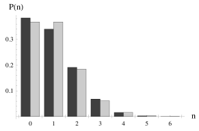
Figure 1: Reconstruction of the photon distribution of a coherent state with $|\alpha|^{2}=1$ (black), and comparison with the theoretical values (light gray). Simulated on/off measurements have been performed with $N=5$ values of $\eta$ ranging between 1% and 5%. The number of experimental measures is $10^{6}$ for each $\eta$. Fidelity of the reconstruction is larger than $F=99\%$.

Finally in Fig. 4 we check the robustness of the ME inference, against errors in the knowledge of the parameters $N_{1}$ and $N_{2}$ that may come from ML estimation in the first step. The quality of the reconstruction has been assessed through fidelity

$$F=\sum_{n}\sqrt{q_{n}\,p_{n}}\>,$$

between the inferred $q_{n}=\langle n|\varrho_{ME}|n\rangle$ and the true $p_{n}=\langle n|\rho|n\rangle$ photon distribution. As it is apparent from the plot the reconstruction’s fidelity remains large if the relative errors on both parameters are about $\pm 5\%$.

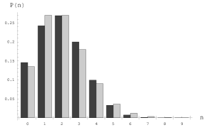
Figure 2: Reconstruction of the photon distribution of a coherent state with $|\alpha|^{2}=2$ (black) and comparison with the theoretical values (light gray). Simulations parameters are the same as in Fig. 1. Fidelity of the reconstruction is larger than $F=99\%$.

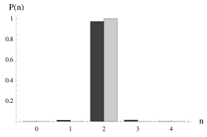
Figure 3: Reconstruction of the photon distribution of the number state $|2\rangle$ (black) and comparison with the theoretical values (light gray). Simulations parameters are the same as in Fig. 1. Fidelity of the reconstruction is $F=98.5\%$.

IV Conclusions

In this paper we have shown that the photon distribution of a light signal $\rho$, with Mandel parameter lower than or equal to its average photon number, can be reconstructed using few measurements collected by a low efficiency avalanche photodetector. The on/off statistics is used in a two steps algorithm, consisting in retrieving the first two moments of the photon distribution via a Maximum-Likelihood estimation, and than inferring the diagonal entries of $\rho$ using of the Maximum Entropy principle. The last step implies the solution of a nonlinear equation in order to shape the statistic to reproduce exactly the moments obtained in the first estimation. Though this last process may be delicate, we showed with simulated experiments that it yields sound results when applied to coherent and number states. Finally we demonstrated that the method exhibits a sufficient robustness against errors deriving from the Maximum-Likelihood estimation.

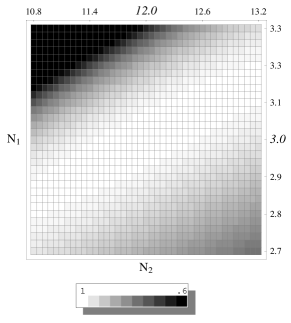
Figure 4: Fidelity of the photon distribution reconstruction for a coherent state $|\alpha|^{2}=3$, as a function of the average photon number $N_{1}$ and its second moment $N_{2}$. The true values for the two parameters are printed in italics. Simulations parameters are the same as in Fig. 1. Notice that the first two entries in the top line are set to 0 because, in these cases, the Mandel parameter $q$ is smaller than -1, so they are not physical states.

References

- (1) C. M. Caves and P. D. Drummond, Rev. Mod. Phys. 66, 481 (1994).
- (2) E. Knill, R. Laflamme, and G. J. Milburn, Nature 409, 46 (2001).
- (3) J. Kim, S. Takeuchi, Y. Yamamoto, and H. H. Hogue, Appl. Phys. Lett. 74, 902 (1999); C. Kurtsiefer, S. Mayer, P. Zarda, and H. Weinfurter, Phys. Rev. Lett. 85, 290 (2000); M. Pelton, C. Santori, J. Vukovic, B. Zhang, G. S. Solomon, J. Plant, and Y. Yamamoto, Phys. Rev. Lett. 89, 233602 (2002).
- (4) G. M. D’Ariano, M. G. A. Paris and M. F. Sacchi, Advances in Imaging and Electron Physics 128, 205 (2003).
- (5) M. Munroe et al., Phys. Rev. A 52, R924 (1995)
- (6) M. Raymer and M. Beck in Quantum states estimation, M. G. A. Paris and J. Řeháček Eds., Lect. Not. Phys. 649 (Springer, Heidelberg, 2004), at press.
- (7) G. M. D’Ariano and M. G. A. Paris, Phys. Lett. A 233 49 (1997).
- (8) D. Mogilevtsev, Opt. Comm. 156, 307 (1998); Acta Phys. Slov. 49, 743 (1999).
- (9) J. ehek, Z. Hradil, O. Haderka, J. Peina, Jr., and M. Hamar, Phys. Rev. A 67, 061801(R) (2003); O. Haderka, M. Hamar and J. Peina, Eur. Phys. Journ. D 28, (2004).
- (10) A. R. Rossi, S. Olivares, M. G. A. Paris, Phys. Rev. A 70, 055801 (2004).
- (11) E. T. Jaynes, Phys. Rev. 106, 620 (1957); 108, 171 (1957).
- (12) V. Buek and G. Adam, Ann. Phys. 245, 37 (1996); V. Buek in Quantum states estimation, M. G. A. Paris and J. Řeháček Eds., Lect. Not. Phys. 649 (Springer, Heidelberg, 2004), p. 189.