Sequential generation of entangled multi-qubit states

Abstract

We consider the deterministic generation of entangled multi-qubit states by the sequential coupling of an ancillary system to initially uncorrelated qubits. We characterize all achievable states in terms of classes of matrix product states and give a recipe for the generation on demand of any multi-qubit state. The proposed methods are suitable for any sequential generation-scheme, though we focus on streams of single photon time-bin qubits emitted by an atom coupled to an optical cavity. We show, in particular, how to generate familiar quantum information states such as W, GHZ, and cluster states, within such a framework.

Entangled multi-qubit states are a valuable resource for the implementation of quantum computation and quantum communication protocols, like distributed quantum computing DQC , quantum cryptography Ekert1991 or quantum secret sharing CGL99 . Using photonic degrees of freedom as qubits, say, polarization states or time-bins of energy eigenstates, has the advantage that photons propagate safely over long distances. Consequently, photonic devices are the most promising systems for quantum communication tasks. For this purpose, a lot of effort has been made in recent years to develop efficient and deterministic single photon sources Law1997 ; Kuhn2002 ; McKeever2004 ; Lange2004 ; Deppe2004 ; Forchel2004 .

Photonic multi-qubit states can be generated by letting a source emit photonic qubits in a sequential manner Gheri2000 . If we do not initialize the source after each step, the created qubits will be in general entangled. Moreover, if we allow for specific operations inside the source before each photon emission, we will be able to create different multi-qubit states at the output. In fact, this is a particular instance of a general sequential generation scheme, where an ancillary system is coupled in turn to a number of initially uncorrelated qubits.

It is the purpose of this paper to provide a complete characterization of all multipartite quantum states achievable within a sequential generation scheme. It turns out that the classes of states attainable with increasing resources are exactly given by the hierarchy of so-called matrix-product states (MPS) Zittartz ; Fannes92 . These states typically appear in the theory of one-dimensional spin systems AKLT , as they are the variational set over which Density Matrix Renormalization Group techniques are carried out DMRG . Thus, our analysis stresses the importance of MPS, since we show that they naturally appear in a completely different and relevant physical context. Moreover, particular instances of low-dimensional MPS, like cluster states Briegel2001 or GHZ states GHZ , are a valuable resource in quantum information VerstCirQC . Conversely, we will provide a recipe for the generation on demand of any multi-qubit state within a sequential generation scheme. Due to the general validity of these results, we will first state and prove them without referring to any particular physical system. This will be then applicable to all sequential setups, like streams of photonic qubits emitted either by a cavity QED (CQED) source Law1997 ; Kuhn2002 ; McKeever2004 ; Lange2004 or by a quantum dot coupled to a microcavity Deppe2004 ; Forchel2004 .

In the second part, we will focus on the physical implementation of these ideas within the realm of CQED. The role of the ancillary system will be performed by a $D$-level atom coupled to a single mode of an optical cavity. The sequentially generated qubits will be time-bin qubits $|0\rangle$ and $|1\rangle$, describing the absence and presence of a photon emitted from the cavity in a certain time interval (see Fig. 1).

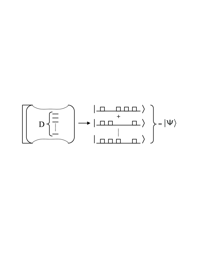
Figure 1: A trapped D-level atom is coupled to a cavity qubit, determined by the energy eigenstates $|0\rangle$ and $|1\rangle$. After arbitrary bipartite source-qubit operations, photonic time-bins are sequentially and coherently emitted at the cavity output, creating a desired entangled multi-qubit stream.

We will concentrate on setups where all intermediate operations are arbitrary unitaries and the ancilla decouples in the last step. The latter enables us to generate pure entangled states in a deterministic manner without the need of measurements. Let ${\cal H}_{\cal A}\simeq\mathbb{C}^{D}$ and ${\cal H}_{\cal B}\simeq\mathbb{C}^{2}$ be the Hilbert spaces characterizing a $D$-dimensional ancillary system and a single qubit (e.g. a time-bin qubit) respectively. In every step of the sequential generation of a multi-qubit state, we consider a unitary time evolution of the joint system ${\cal H}_{\cal A}\otimes{\cal H}_{\cal B}$. Assuming that each qubit is initially in the state $|0\rangle$ (i.e., the time-bin is empty), we disregard the qubit at the input and write the evolution in the form of an isometry $V:{\cal H}_{\cal A}\rightarrow{\cal H}_{\cal A}\otimes{\cal H}_{\cal B}$. Expressing the latter in terms of a basis $V=\sum_{i,\alpha,\beta}V_{\alpha,\beta}^{i}|\alpha,i\rangle\langle\beta|$, the isometry condition reads $\sum_{i=0}^{1}V^{i\dagger}V^{i}=\mbox{$1{\bf l}$}$, where each $V^{i}$ is a $D\times D$ matrix. We choose a basis where $\{|\alpha\rangle,|\beta\rangle\}$ are any of the $D$ ancillary levels. If we now apply successively $n$, not necessarily identical, operations of this form to an initial state $|\varphi_{I}\rangle\in{\cal H}_{\cal A}$, we obtain the state

$$|\Psi\rangle=V_{[n]}\ldots V_{[2]}V_{[1]}|\varphi_{I}\rangle\;.$$ (1)

Here, and in the following, indices in squared brackets represent the steps in the generation sequence. The $n$ generated qubits are in general entangled with the ancilla as well as among themselves. Assuming that in the last step the ancilla decouples from the system, such that $|\Psi\rangle=|\varphi_{F}\rangle\otimes|\psi\rangle$, we are left with the $n$-qubit state

$$|\psi\rangle=\sum_{i_{1}\ldots i_{n}=0}^{1}\langle\varphi_{F}|V_{[n]}^{i_{n}}\ldots V_{[1]}^{i_{1}}|\varphi_{I}\rangle\;|i_{n},\ldots,i_{1}\rangle.$$ (2)

States of this form are called matrix-product states (MPS) Zittartz ; Fannes92 , and play a crucial role in the theory of one-dimensional spin systems. Equation (2) shows that all sequentially generated multi-qubit states, arising from a $D$-dimensional ancillary system ${\cal H}_{\cal A}$, are instances of MPS with $D\times D$ matrices $V^{i}$ and open boundary conditions specified by $|\varphi_{I}\rangle$ and $|\varphi_{F}\rangle$. We will now prove that the converse is also true, i.e., that every MPS of the form

$$|\tilde{\psi}\rangle=\langle\tilde{\varphi}_{F}|\tilde{V}_{[n]}\ldots\tilde{V}_{[1]}|\tilde{\varphi}_{I}\rangle,$$ (3)

with arbitrary maps $\tilde{V}_{[k]}:{\cal H}_{\cal A}\rightarrow{\cal H}_{\cal A}\otimes{\cal H}_{\cal B}$, can be generated by isometries of the same dimension, and such that the ancillary system decouples in the last step. Since every state has a MPS representation, this is at the same time a general recipe for its sequential generation. The idea of the proof is an explicit construction of all involved isometries by subsequent application of singular value decompositions (SVD). We start by writing $\langle\tilde{\varphi}_{F}|\tilde{V}_{[n]}=V_{[n]}^{\prime}M_{[n]}$, where the $2\times 2$ matrix $V_{[n]}^{\prime}$ is the left unitary in the SVD and $M_{[n]}$ is the remaining part. The recipe for constructing the isometries is the induction

$$\big{(}M_{[k]}\otimes\mbox{$1{\bf l}$}_{2}\big{)}\tilde{V}_{[k-1]}=V_{[k-1]}^{\prime}M_{[k-1]},$$ (4)

where the isometry $V_{[k-1]}^{\prime}$ is constructed from the SVD of the left hand side, and $M_{[k-1]}$ is always chosen to be the remaining part. After $n$ applications of Eq. (4) in Eq. (3), from left to right, we set $|\varphi_{I}\rangle=M_{[1]}|\tilde{\varphi}_{I}\rangle$, producing

$$|\tilde{\psi}\rangle=V_{[n]}^{\prime}\ldots V_{[1]}^{\prime}|\varphi_{I}\rangle.$$ (5)

Simple rank considerations show that $V_{[n-k]}^{\prime}$ has dimension $2\min{[D,2^{k}]}\times\min{[D,2^{k+1}]}$. In particular, every $V_{[k]}^{\prime}$ could be embedded into an isometry $V_{[k]}$ of dimension $2D\times D$. Physically, this just means we would have redundant ancillary levels that we need not to use. Finally, decoupling the ancilla in the last step is guaranteed by the fact that, after the application of $V_{[n-1]}$, merely two levels of ${\cal H}_{\cal A}$ are yet occupied, and can be mapped entirely onto the system ${\cal H}_{\cal B}$. This is precisely the action of $V_{[n]}$ through its embedded unitary $V_{[n]}^{\prime}$.

This proves the equivalence of two sets of $n$-qubit states, which are described either as $D$-dimensional MPS with open boundary conditions, or as states that are generated sequentially and isometrically via a $D$-dimensional ancillary system which decouples in the last step. Motivated by current cavity QED setups, we will now provide a third equivalent characterization, namely, a set of multi-qubit states that are sequentially generated by a source consisting of a $2D$-level atom. In contrast to the first sequential scheme, the latter will not require arbitrary isometries.

Consider an atomic system with $D$ states $|a_{i}\rangle$ and $D$ states $|b_{i}\rangle$, so that ${\cal H}_{\cal A}={\cal H}_{a}\oplus{\cal H}_{b}\simeq\mathbb{C}^{d}\otimes\mathbb{C}^{2}$. That is, we will write $|\varphi\rangle|1\rangle$ for a superposition of $|a_{i}\rangle$ states, whereas $|\varphi\rangle|0\rangle$ corresponds to a superposition of $|b_{i}\rangle$ states. Since the last qubit marks the atomic level, whether it belongs to the $|a_{i}\rangle$ or to the $|b_{i}\rangle$ subspace, we will refer to it as the tag-qubit and write ${\cal H}_{\cal A}={\cal H}_{{\cal A}^{\prime}}\otimes{\cal H}_{\cal T}$. Now consider the atomic transitions from each $|a_{i}\rangle$ state to its respective $|b_{i}\rangle$ state accompanied by the generation of a photon in a certain time-bin. This is described by a unitary evolution, since now called “D-standard map”, of the form

$$T:\;|\varphi\rangle_{{\cal A}^{\prime}}|1\rangle_{\cal T}|0\rangle_{\cal B} \mapsto |\varphi\rangle_{{\cal A}^{\prime}}|0\rangle_{\cal T}|1\rangle_{\cal B}\;,$$

$$|\varphi\rangle_{{\cal A}^{\prime}}|0\rangle_{\cal T}|0\rangle_{\cal B} \mapsto |\varphi\rangle_{{\cal A}^{\prime}}|0\rangle_{\cal T}|0\rangle_{\cal B}\;.$$ (6)

Hence, $T$ effectively interchanges the tag-qubit with the time-bin qubit. If, additionally, arbitrary atomic unitaries $U_{{\cal A}}$ are allowed at any time, we can exploit the swap caused by $T$ in order to generate the operation

$$V|\varphi\rangle=\langle 0|_{\cal T}T\Big{(}U_{{\cal A}}\big{(}|\varphi\rangle_{{\cal A}^{\prime}}|0\rangle_{\cal T}\big{)}|0\rangle_{\cal B}\Big{)}\;,$$ (7)

which is the most general isometry $V:{\cal H}_{{\cal A}^{\prime}}\rightarrow{\cal H}_{{\cal A}^{\prime}}\otimes{\cal H}_{\cal B}$. Therefore, the so generated $n$-qubit states include all possible states arising from subsequent applications of $2D\times D$-dimensional isometries. On the other hand, they are a subset of the MPS in Eq. (3) with arbitrary $2D\times D$-dimensional maps, assuming that the atom decouples at the end. Hence, these three sets are all equivalent.

Now, we show how these results can be applied in the realm of cavity QED, where an atom is trapped inside a high-$Q$ optical cavity, and we aim at generating multi-photon entangled states. A laser may excite the atom, producing subsequently a photon in the cavity mode, which, after some time, is emitted outside the cavity (Fig. 1). We consider two different scenarios, corresponding to the two families of states considered above. First, we may have fast and complete access to the atom-cavity system. In consequence, after the implementation of the desired isometry in each step, we should wait until the photon leaks out of the cavity before starting the next step. In this case, according to the analysis above, we will be able to produce arbitrary $D$-dimensional MPS with $D$ equal to the number of involved atomic levels. Second, we may have a 2$D$–level atom ($D$ $|a_{i}\rangle$ levels and $D$ $|b_{i}\rangle$ levels) and two kind of operations: (i) fast arbitrary operations which allow us to manipulate at will all atomic levels; (ii) an operation which maps each $|a_{i}\rangle$ state to its corresponding $|b_{i}\rangle$ state while creating a single cavity photon, allowing a taylored output. Here, we will also be able to produce arbitrary $D$-dimensional MPS.

In the following, we will illustrate the above statements with a specific example which is based on present cavity QED experiments Kuhn2002 ; McKeever2004 ; Lange2004 . We consider a three–level atom coupled to a single cavity mode in the strong-coupling regime. An external laser field drives the transition from level $|a\rangle$ to the upper level $|u\rangle$ with coupling strength $\Omega_{0}$, and the cavity mode drives the transition between $|u\rangle$ and level $|b\rangle$ with coupling strength $g$, in a typical $\Lambda$ configuration [see Fig. 2(a)]. We choose the detunings $\Delta$, with $|\Delta|\gg\{g,\Omega_{0}\}$, and assume that the cavity decay rate $\kappa$ is smaller than any other frequency in the problem, so that we can ignore cavity damping during the atom-cavity manipulations. By eliminating level $|u\rangle$, we remain with an effective $D=2$ atomic system plus the cavity mode. We will show how, by controlling the laser frequency and intensity, it is possible to generate arbitrary $2$-dimensional MPS. Note that, by allowing the manipulation of $D$ effective atomic levels, it is straightforward to extend these results to the generation of $D$-dimensional MPS.

According to the results presented above, we just have to show that we can implement any isometry $V:{\cal H}_{\cal A}\rightarrow{\cal H}_{\cal A}\otimes{\cal H}_{\cal B}$. In fact, we will show how it is possible to implement arbitrary operations on the atomic qubit and the $\sqrt{SWAP}$ operation on the atom-cavity system, which suffice to generate any isometry $V$ (since they give rise to a universal set of gates for the two qubit system Nielsen2000 ). The atomic qubit can be manipulated at will using a Raman laser system, as it is normally done with trapped ions NIST ; Innsbruck . In order to implement the $\sqrt{SWAP}$, we notice that the atom-cavity coupling is described in terms of the Jaynes–Cummings model [see Fig. 2(b)], where the coupling constant $\Omega_{0}$ is controlled by the laser. Thus, application of laser pulses with the appropriate duration and phase Innsbruck ; SelectiveCQED will implement the unitary operation $U=e^{-iG}$, where generator $G=(|a,0\rangle\langle b,1|+{\rm H.c.})\pi/4$, which corresponds to the desired $\sqrt{SWAP}$ operation. In order to generalize this scheme to an arbitrary $D$-level system, we notice that we can view the atom as a set of $M$ qubits (with $D\leq 2^{M}$). Thus, if we are able to perform arbitrary atomic operations, together with the $\sqrt{SWAP}$ operation on two specific atomic levels as explained above, we can then implement a universal set of gates and, in consequence, any arbitrary isometry.

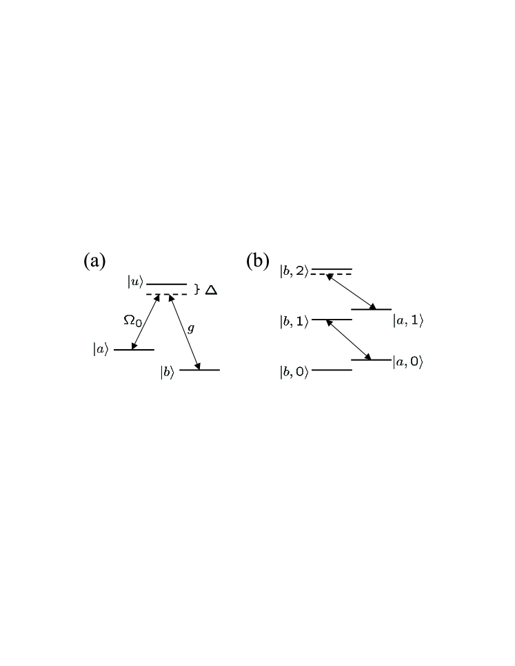
Figure 2: (a) Atomic level structure: levels $|a\rangle$ ($|b\rangle$) and $|u\rangle$ are coupled by a laser (cavity mode) off resonance. (b) After adiabatic elimination of the upper state $|u\rangle$, we are left with a Jaynes–Cummings type of Hamiltonian, where states $|a,n\rangle$ and $|b,n+1\rangle$ are coupled. Both, the energy difference of those levels and the corresponding Rabi frequency depends on $n$. The reason for the first is the AC–Stark shift, whereas the second is due to the Jaynes–Cummings coupling.

In the rest of the paper, we will use another setup which is closely related to current experiments Kuhn2002 ; McKeever2004 ; Lange2004 and optimizes our second method for MPS generation. In this frame, we will show how to generate familiar multi-qubit states like $W$ Wstates , $GHZ$ GHZ , and cluster states Briegel2001 , which are all MPS with $D=2$ VerstCirQC .

For the purpose, we consider an atom with three effective levels $\{|a\rangle,|b_{1}\rangle,|b_{2}\rangle\}$ trapped inside an optical cavity. With the help of a laser beam, state $|a\rangle$ is mapped to the internal state $|b_{1}\rangle$, and a photon is generated, whereas the other states remain unchanged. This physical process is described by the map

$$M_{{\cal A}{\cal B}}:\;|a\rangle \mapsto |b_{1}\rangle|1\rangle\;,$$

$$|b_{1}\rangle \mapsto |b_{1}\rangle|0\rangle\;,$$

$$|b_{2}\rangle \mapsto |b_{2}\rangle|0\rangle\;,$$ (8)

and can be realized with the techniques used in Kuhn2002 ; McKeever2004 ; Lange2004 . After the application of this process, an arbitrary operation is applied to the atom, which can be performed by using Raman lasers. The photonic states that are generated after several applications are those MPS where the isometries are given by $V_{[i]}=M_{{\cal A}{\cal B}}U_{\cal A}^{[i]}$, with ${i=1,\dots,n}$, $U_{\cal A}^{[i]}$ being arbitrary unitary atomic operators.

For example, to generate a W-type state of the form

$$|\psi_{\rm W}\rangle = e^{i\Phi_{1}}\sin\Theta_{1}|0...01\rangle+\cos\Theta_{1}e^{i\Phi_{2}}\sin\Theta_{2}|0...010\rangle$$ (9)

$$+...+\cos\Theta_{1}...\cos\Theta_{n-2}e^{i\Phi_{n-1}}\sin\Theta_{n-1}|010...0\rangle$$

$$+\cos\Theta_{1}...\cos\Theta_{n-1}|10...0\rangle,$$

we choose the initial atomic state $|\varphi_{I}\rangle=|b_{2}\rangle$ and operations $U_{\cal A}^{[i]}=U_{a{b_{2}}}^{b_{1}}(\Phi_{i},\Theta_{i})$, with $i=1,\dots,n-1$, where

$$U_{kl}^{m}(\Phi_{i},\Theta_{i}) \!\!\!\!\!=\!\!\!\! \cos\Theta_{i}|k\rangle\langle k|+\cos\Theta_{i}|l\rangle\langle l|+e^{i\Phi_{i}}\!\sin\Theta_{i}|k\rangle\langle l|$$ (10)

$$-e^{-i\Phi_{i}}\sin\Theta_{i}|l\rangle\langle k|+|m\rangle\langle m|,$$

and $\{k,l,m\}=\{a,b_{1},b_{2}\}$. To decouple the atom from the photon state, we choose the last atomic operation $U_{\cal A}^{[n]}=U_{a{b_{2}}}^{b_{1}}(0,\pi/2)$ and, after the last map $M_{{\cal A}{\cal B}}$, the decoupled atom will be in state $|b_{1}\rangle$.

To produce a GHZ-type state in similar way, we choose $|\varphi_{I}\rangle=|a\rangle$, $U_{\cal A}^{[1]}=U_{a{b_{2}}}^{b_{1}}(\Phi_{1},\Theta_{1})$, $U_{\cal A}^{[i]}=U_{a{b_{1}}}^{b_{2}}(0,\pi/2)$, with $i=2,\dots,n-1$, and $U_{\cal A}^{[n]}=U_{{b_{1}}{b_{2}}}^{a}(0,\pi/2)U_{a{b_{1}}}^{b_{2}}(0,\pi/2)$.

For generating cluster states, we choose $|\varphi_{I}\rangle=|b_{2}\rangle$, $U_{\cal A}^{[i]}=U_{a{b_{2}}}^{b_{1}}(\Phi_{i},\Theta_{i})U_{a{b_{1}}}^{b_{2}}(0,\pi/2)$, with $i=1,\dots,n-1$, and $U_{\cal A}^{[n]}=U_{a{b_{1}}}^{b_{2}}(\Phi_{n},\Theta_{n})U_{{b_{1}}{b_{2}}}^{a}(0,\pi/2)U_{a{b_{1}}}^{b_{2}}(0,\pi/2)$, obtaining

$$|\psi\rangle=\bigotimes_{i=1}^{n}\left(O_{i-1}^{0}|0\rangle_{i}+O_{i-1}^{1}|1\rangle_{i}\right),$$ (11)

where $O^{0}_{i-1}=\cos\Theta_{i}|0\rangle_{i-1}\langle 0|-e^{-i\Phi_{i}}\sin\Theta_{i}|1\rangle_{i-1}\langle 1|$ and $O^{1}_{i-1}=e^{i\Phi_{i}}\sin\Theta_{i}|0\rangle_{i-1}\langle 0|+\cos\Theta_{i}|1\rangle_{i-1}\langle 1|$, with ${i=2,\dots,n-1}$. Operators $O_{i-1}^{0}$ and $O_{i-1}^{1}$ act on the nearest neighbor-qubit $i-1$ under the assumption $O_{0}^{0}\equiv\cos\Theta_{1}$ and $O_{0}^{1}\equiv e^{i\Phi_{1}}\sin\Theta_{1}$. If one chooses $\Phi_{i}=0$ and $\Theta_{i}=\pi/4$ this leads to the cluster states defined by

$$|\psi_{\rm cl}\rangle=\frac{1}{2^{n/2}}\bigotimes_{i=1}^{n}\left(\sigma^{z}_{i-1}|0\rangle_{i}+|1\rangle_{i}\right)\,\,,\,\,{\rm with}\,\,\,\sigma^{z}_{0}\equiv 1.$$ (12)

The formalism presented here is also valid for other types of single-photon sources, in the context of cavity QED or quantum dots. For example, it could be extended to characterize the polarization-entangled multi-qubit photon states generated by an analogous cavity QED photon source Gheri2000 . In fact, the presented ideas and proofs apply to any multi-qudit state with ${\cal H}_{{\cal B}}\simeq\mathbb{C}^{d}$ that is generated sequentially by a $D$-dimensional source.

In a wider scope, we have established a formalism describing a general sequential quantum factory, where the source is able to perform arbitrary unitary source-qudit operations before each qudit leaves. Apart from the multiphoton states, the present formalism applies also to many other physical scenarios: (a) to coherent microwave cavity QED experiments Haroche , where atoms sequentially cross a cavity, and thus the outcoming atoms end up in a MPS with the dimensions given by the effective number of states used in the cavity mode; (b) a light pulse crossing several atomic ensembles Polzik2003 , which will be left in a matrix product Gaussian state Norbert ; (c) trapped ion experiments where each ion interacts sequentially with a collective mode of the motion NIST ; Innsbruck ; CiracZoller . Note also that one can include dissipation in the present formalism, by replacing MPS by matrix product density operators  Fannes92 ; MPDO . This description applies, for example, to the micromaser setup  Walther2001 and other realistic scenarios.

C.S. wants to thank K. Hammerer for useful discussions. This work was supported by EU through RESQ project and the ”Kompetenznetzwerk Quanteninformationsverarbeitung der Bayerischen Staatsregierung”.

References

- (1) L. G. Grover, quant-ph/9704012; J. I. Cirac, A. K. Ekert, S. F. Huelga, and C. Macchiavello, Phys. Rev. A 59, 4249 (1999).
- (2) A. K. Ekert, Phys. Rev. Lett. 67, 661 (1991).
- (3) R. Cleve, D. Gottesmann, and H.-K. Lo, Phys. Rev. Lett. 83, 648 (1999).
- (4) C. K. Law and H. J. Kimble, J. Mod. Opt. 44, 2067-2074 (1997).
- (5) A. Kuhn, M. Hennrich, and G. Rempe, Phys. Rev. Lett. 89, 067901 (2002).
- (6) J. McKeever, A. Boca, A. D. Boozer, R. Miller, J. R. Buck, A. Kuzmich, and H. J. Kimble, Science 303, 1992 (2004).
- (7) M. Keller, B. Lange, K. Hayasaka, W. Lange, and H. Walther, Nature 431, 1075 (2004).
- (8) T. Yoshie, A. Scherer, J. Hendrickson, G. Khitrova, H. M. Gibbs, G. Rupper, C. Ell, O. B. Shchekin, and D. G. Deppe, Nature 432, 200 (2004).
- (9) J. P. Reithmaier, G. Sek, A. Loffler, C. Hofmann, S. Kuhn, S. Reitzenstein, L. V. Keldysh, V. D. Kulakovskii, T. L. Reinecke, and A. Forchel, Nature 432, 197 (2004).
- (10) K.M. Gheri, C. Saavedra, P. Törm, J. I.. Cirac and P. Zoller, Phys. Rev. A 58, R2627 (1998);C. Saavedra, K. M. Gheri, P. Törmä, J. I. Cirac, and P. Zoller, Phys. Rev. A 61, 062311 (2000).
- (11) A. Klümper, A. Schadschneider, and J. Zittartz, J. Phys. A 24, L955 (1991); Z. Phys. B 87, 281 (1992); Europhys. Lett. 24, 293 (1993).
- (12) M. Fannes, B. Nachtergaele, and R. F. Werner, Comm. Math. Phys. 144, 443 (1992).
- (13) I. Affleck et al., Commun. Math. Phys. 115, 477 (1988).
- (14) S. Östlund and S. Rommer, Phys. Rev. Lett. 75, 3537 (1995).
- (15) H. J. Briegel and R. Raussendorf, Phys. Rev. Lett. 86, 910 (2001).
- (16) D. M. Greenberger, M. Horne, and A. Zeilinger, in Bell’s Theorem, Quantum Theory, and Conceptions of the Universe, M. Kafatos, Ed. (Kluwer, Dordrecht 1989) pp. 69-72.
- (17) F. Verstraete and J. I. Cirac, Phys. Rev. A 70, 060302 (2004)
- (18) M. Nielsen and I. Chuang, Quantum computation and quantum information, Cambridge Univ. Press (2000).
- (19) D. Kielpinski, C. Monroe, and D. J. Wineland, Nature (London) 417, 709 (2002).
- (20) S. Gulde, M. Riebe, G. P. T. Lancaster, C. Becher, J. Eschner, H. Häffner, F. Schmidt-Kaler, I. L. Chuang, and R. Blatt, Nature (London) 421, 48 (2003).
- (21) M. França Santos, E. Solano, and R. L. de Matos Filho, Phys. Rev. Lett. 87, 093601 (2001).
- (22) W. Dür, G. Vidal, and J. I. Cirac, Phys. Rev. A 62, 062314 (2000).
- (23) A. Rauschenbeutel, G. Nogues, S. Osnaghi, P. Bertet, M. Brune, J.-M. Raimond, and S. Haroche, Science 288, 2024 (2000).
- (24) B. Julsgaard, C. Schori, J.L. Sørensen, E.S. Polzik., Quant. Inform. and Comp., spec. issue 3, 518 (2003).
- (25) N. Schuch, M. Wolf, F. Verstraete, and J.I. Cirac (in preparation).
- (26) J. I. Cirac and P. Zoller, Phys. Rev. Lett. 74, 4091 (1995).
- (27) F. Verstraete, J. J. Garcia-Ripoll, and J. I. Cirac, Phys. Rev. Lett. 93, 207204 (2004); M. Zwolak and G. Vidal, ibid, 207208 (2004) .
- (28) S. Brattke, B. T. H. Varcoe, and H. Walther, Phys. Rev. Lett. 86, 3534 (2001).