Hamiltonian Formalism of Game Theory

Abstract

A new representation of Game Theory is developed in this paper. State of players is represented by a density matrix, and payoff function is a set of hermitian operators, which when applied onto the density matrix gives the payoff of players. By this formalism, a new way to find the equilibria of games is given by generalizing the thermodynamical evolutionary process leading to equilibrium in Statistical Mechanics. And in this formalism, when quantum objects instead of classical objects are used as the objects in the game, it naturally leads to the Traditional Quantum Game, but with a slight difference in the definition of strategy state of players: the probability distribution is replaced with a density matrix. Further more, both games of correlated and independent players can be represented in this single framework, while traditionally, they are treated separately by Non-cooperative Game Theory and Coalitional Game Theory. Because the density matrix is used as state of players, besides classical correlated strategy, quantum entangled states can also be used as strategies, which is an entanglement of strategies between players, and it is different with the entanglement of objects’ states as in the Traditional Quantum Game. At last, in the form of density matrix, a class of quantum games, where the payoff matrixes are commutative, can be reduced into classical games. In this sense, it will put the classical game as a special case of our quantum game.

Key Words: Game Theory, Quantum Game Theory, Quantum Mechanics, Hilbert Space, Probability Theory, Statistical Mechanics

Pacs: 02.50.Le, 03.67.-a, 03.65.Yz

1 Introduction

For static non-cooperative games, theoretically Nash Theorem gives a closed conclusion on the existence of equilibrium. However, the way to calculate the equilibrium of general games are still open, and so far the existing methods seem not very general.

On the other hand, in Physics, we do have similar situations and solutions, and they provide prototypes to deal with the problem above. In Statistical Mechanics, principally or at least practically, we have no dynamical evolutionary process, or say, by first principle, leading to thermal equilibrium, but the definition of thermal equilibrium is definitely clear, and we do have some pseudo-dynamical processes such as the Liouville-von Neumann equation for relevant partial system[1] or artificial man-made evolutionary processes, such as Metropolis Method[2], giving the correct thermal equilibrium in a quite general sense. Now we want to apply this experience onto Game Theory.

The basis of such application is the same mathematical form should be used in both Physics and Game Theory. Here, we choose density matrix as this basis. The equilibrium of a statistical system is defined as

$$P\left(\vec{x};\beta\right)=\frac{1}{Z}e^{-\beta E\left(\vec{x}\right)},$$ (1)

where $\vec{x}$ is the dynamical variable, usually including general position and general momentum, and $Z$ is the normalized constant,

$$Z=\int d\vec{x}e^{-\beta E\left(\vec{x}\right)}.$$ (2)

Or for a quantum statistical system,

$$P\left(E_{n};\beta\right)=\frac{1}{Z}e^{-\beta E_{n}},$$ (3)

where

$$Z=\sum_{n}e^{-\beta E_{n}},$$ (4)

and $n$ is the complete good quantum number for this system. The above definitions can be unified as an operator form, that

$$\hat{\rho}\left(\beta\right)=\frac{1}{Z}e^{-\beta\hat{H}},$$ (5)

and

$$Z=\int d\vec{x}d\vec{x}^{\prime}\left<\vec{x}\right|e^{-\beta\hat{H}}\left|\vec{x}^{\prime}\right>.$$ (6)

The way to use an operator form for classical systems may seem wired even for readers in Physics. However, it’s quite trivial if we regard classical systems as systems always having trivial eigenstates with eigenvalues $\vec{x}$, that

$$\hat{H}\left|\vec{x}\right>=E\left(\vec{x}\right)\left|\vec{x}\right>,$$ (7)

and with normalization

$$\left<\vec{x}^{\prime}\left|\vec{x}\right.\right>=\delta\left(\vec{x}-\vec{x}^{\prime}\right).$$ (8)

Such unification of notation brings nothing new into Physics, but in this paper, the operator-form formalism unifies all the formulas so that easy to apply onto both classical and quantum game. It’s helpful to make an immediate application of this notation, that the operator form of classical thermal equilibrium can be written as

$$\begin{array}[]{ccc}\hat{\rho}^{classical}\left(\beta\right)&=&\frac{1}{Z}\int d\vec{x}d\vec{x}^{\prime}\left|\vec{x}^{\prime}\right>\left<\vec{x}^{\prime}\right|e^{-\beta\hat{H}}\left|\vec{x}\right>\left<\vec{x}\right|\\ \\ &=&\frac{1}{Z}\int d\vec{x}d\vec{x}^{\prime}\left|\vec{x}^{\prime}\right>e^{-\beta E\left(\vec{x}\right)}\delta\left(\vec{x}^{\prime}-\vec{x}\right)\left<\vec{x}\right|\\ \\ &=&\frac{1}{Z}\int d\vec{x}\left|\vec{x}\right>e^{-\beta E\left(\vec{x}\right)}\left<\vec{x}\right|.\end{array}$$ (9)

It’s important to notice the general character that for a classical system that only the diagonal terms exist, while for a quantum system, it depends on the basis. Especially, for basis $\left\{\left|x\right>\right\}$, the eigenvectors of position vector $\hat{X}$, usually, the density matrix has the off-diagonal terms.

Then all thermal dynamical quantities should be averaged over the whole space from dynamical variables according to this Boltzman distribution. However, for a many-body system, such summation over the whole space is not an easy mission. So average over a sampling of this distribution is used to replace the whole space summation. The idea is if we have the dynamical process driving the system into thermal equilibrium, then we can just start from an arbitrary initial state, and then let the system evolute according to the dynamical process. After some long time, we record the trajectory, and use the states on this trajectory as samples of equilibrium states. Then, the average can be done on those samples. Unfortunately, principally we don’t even have such dynamical process. However, the artificial man-made evolutionary process, such as Metropolis Method, survives this idea. The idea of Metropolis Method[2] is to define an evolutionary process also leading to the right thermal equilibrium not from first principle such as dynamical equations, but from the detailed balance principle, which is

$$\frac{w\left(\vec{x}\rightarrow\vec{x}^{\prime}\right)}{w\left(\vec{x}^{\prime}\rightarrow\vec{x}\right)}=\frac{e^{-\beta E\left(\vec{x}^{\prime}\right)}}{e^{-\beta E\left(\vec{x}\right)}}.$$ (10)

This will give us the transition rate between states $\vec{x}$ and $\vec{x}^{\prime}$ with the help of other arguments[2]. Then, the system can start from an arbitrary initial state, and at every time step, according to the probability given by the transition rate, it moves onto or rejects a new test state randomly chosen from all other states. For a short summery, whatever the detail of the evolutionary process will be, the conclusion is, for a system described by Hamiltonian, we do have some methods to get the thermal equilibrium.

Now we apply this idea onto games. The first requirement is the system should be described by a Hamiltonian such as a hermitian operator $\hat{H}$. And the state of system should be represented by a vector $\vec{x}$ or $\left|\vec{x}\right>$. How far away does the current formalism of Game Theory leave from those two requirements? Traditionally, the description of system-level state does not exist but only a set of states for every single player, which are a set of probability distributions over their own strategy spaces. Or, say, in non-cooperative static game, state of player is $\left\{\rho^{i}\right\}$, where every $\rho^{i}$ is a probability distribution, such as

$$p^{i}\left(s^{i}_{l}\right)=p^{i}_{l},$$ (11)

or in our notation,

$$\rho^{i}=\sum_{l}p^{i}_{l}\left|s^{i}_{l}\right>\left<s^{i}_{l}\right|.$$ (12)

It’s natural to form a system-level distribution for $N$-player game as

$$P\left(s^{1}_{l_{1}},s^{2}_{l_{2}},\dots,s^{N}_{l_{N}}\right)=p^{1}_{l_{1}}p^{2}_{l_{2}}\dots p^{N}_{l_{N}}.$$ (13)

or in our notation,

$$\rho^{S}=\prod_{i=1}^{N}\rho^{i}=\sum_{\left\{l_{i}\right\}}p^{1}_{l_{1}}p^{2}_{l_{2}}\dots p^{N}_{l_{N}}\left|s^{1}_{l_{1}},s^{2}_{l_{2}},\dots,s^{N}_{l_{N}}\right>\left<s^{1}_{l_{1}},s^{2}_{l_{2}},\dots,s^{N}_{l_{N}}\right|.$$ (14)

Therefore, the state seems not very far away from the requirement, at least we already have the vector form as $\left(s^{1}_{l_{1}},\dots,s^{N}_{l_{N}}\right)^{T}$, or $\left|s^{1}_{l_{1}},\dots,s^{N}_{l_{N}}\right>$. The main problem is at the payoff function.

Traditionally, in a $N$-player game, every player is assigned a payoff function $M^{i}$, which linearly maps $N$ vectors into a real number, or technically speaking $M^{i}$ is a $\left(0,N\right)$-tensor. However, an hermitian operator $\hat{H}$ is required to be a $\left(1,1\right)$-tensor, which maps a left vector and a right vector into a real number. Constructing $H^{i}$ from $M^{i}$ will be a significant step in our formalism. This will be done in section $\S$3. After we get $H^{i}$, we will see it’s truly hermitian.

The main task of this paper is to develop a Hamiltonian Formalism for Game Theory. For classical game, it’s mainly from $M^{i}$ to $H^{i}$. And then we will show the value of such new representation. Another thread leading to this paper, is to consider the game-theory problem that when we replace the classical object with a quantum object, what we need to do for the general framework? Here the object refers to the object which the strategies of the game apply on, such as the coin in the Penny Flipping Game (PFG).

Game Theory[3] is to predict the strategy of all players in a game, no matter a classical object or a quantum object is used as the game object which strategies acts on. For example, when we talk about $2$-player PFG, the object is a coin, which is a classical object with two basic states $\left\{1(head),-1(tail)\right\}$, so the strategies we can use are Non-flip and Flip. We denote them as $I,X$ respectively, for some reason will be known soon. So the strategy state of every player is a probability distribution over $\left\{I,X\right\}$. Now, consider a quantum object, a $\frac{1}{2}$-spin instead of a penny. A spin has more states than a penny. The difference is a penny only has probability combination over $\left\{1,-1\right\}$ states, while a spin has coherent combination over $\left\{1,-1\right\}$ states. Or technically, we say, a general state of a spin is

$$\left|spin\right>=\alpha\left|+1\right>+\beta\left|-1\right>,$$ (15)

with constrain, $\alpha^{*}\alpha+\beta^{*}\beta=1$ while a penny state is a probability distribution such as

$$p\left(+1\right)=p^{+},p\left(-1\right)=p^{-},$$ (16)

with constrain, $p^{+}+p^{-}=1$. It’s easier to distinguish those two objects by using density matrix,

$$\rho^{spin}=\alpha^{*}\alpha\left|+1\right>\left<+1\right|+\beta^{*}\alpha\left|+1\right>\left<-1\right|+\alpha^{*}\beta\left|-1\right>\left<+1\right|+\beta^{*}\beta\left|-1\right>\left<-1\right|,$$ (17)

while

$$\rho^{penny}=p^{+}\left|+1\right>\left<+1\right|+p^{-}\left|-1\right>\left<-1\right|.$$ (18)

The way that we use density matrix to describe state of classical object recalls the same treatment and understanding mentioned above as in equ(9). We see that for classical object, at least the density matrix provides equivalent information with probability distribution. Because of these extra states, the strategy (operator) space over quantum object is also larger than the one over the corresponding classical object. Here, explicitly, for spin, we have four basic strategies (operators): $I,X,Y,Z$ v.s. $I,X$ for penny. Here $I,X,Y,Z$ refers to identity matrix, and three Pauli matrixes,

$$\begin{array}[]{cccc}I=\left[\begin{array}[]{cc}1&0\\ 0&1\end{array}\right]&X=\left[\begin{array}[]{cc}0&1\\ 1&0\end{array}\right]&Y=\left[\begin{array}[]{cc}0&-i\\ i&0\end{array}\right]&Z=\left[\begin{array}[]{cc}1&0\\ 0&-1\end{array}\right]\end{array},$$ (19)

It’s easy to see that $X$ exchanges the states $\left(+1,-1\right)$ and $I$ keeps the states. A general quantum operator can be expressed as

$$s^{i}=e^{i\alpha}\left(\cos{\frac{\gamma}{2}}\cos{\frac{\beta+\delta}{2}}I+i\sin{\frac{\gamma}{2}}\sin{\frac{\beta-\delta}{2}}X-i\sin{\frac{\gamma}{2}}\cos{\frac{\beta-\delta}{2}}Y-i\cos{\frac{\gamma}{2}}\sin{\frac{\beta+\delta}{2}}Z\right),$$ (20)

where $\alpha,\beta,\gamma,\delta$ are real number[4]. Therefore, the classical probability distribution over $I,X$ for classical game should be replaced by a quantum probability distribution over $I,X,Y,Z$ for quantum game.

However, there are two ways to do this generalization. One is to consider a classical probability distribution over all quantum operators. This was widely used in [5, 6, 7, 8], where the distribution will be a classical probability combination as,

$$\rho^{player}_{Cl}=\sum_{\alpha,\beta,\gamma,\delta}p^{player}\left(\alpha,\beta,\gamma,\delta\right)\left|s\right>\left<s\right|.$$ (21)

We will discuss this in more details in section $\S$4.1. Another way is a density matrix on the basis of $\left\{I,X,Y,Z\right\}$, so that

$$\rho^{player}_{Qu}=\sum_{\lambda,\sigma\in\left\{I,X,Y,Z\right\}}\rho^{player}_{\lambda\sigma}\left|\lambda\right>\left<\sigma\right|.$$ (22)

In section $\S$4.1, we will compare those two and conclude they are different, and hopefully give a conclusion that the second definition $\rho^{player}_{Qu}$ should be used.

Because the system-level state is our fundamental dynamical variable, this representation is born as a way to deal with both non-cooperative and coalitional games. So section $\S$4.2 is devoted to discuss about correlated strategy state between players. Here correlation refers to both classically correlation and entanglement in quantum sense. We mainly want to distinguish the difference between the entanglement coming from the object states when there are more than one sub-objects in our quantum game, and the entanglement coming from correlated players. In that section, we will also show a thread on the way to generalize our formalism to explicitly include Coalitional Game Theory.

In the last part of this paper, we come back to our starting point, whether this new formalism helps to find the Nash Equilibria. We have not got a general conclusion yet, so just one representative example is discussed. Also we will put classical game as a limit situation of our quantum game when the payoff matrixes $\left\{H^{i}\right\}$ have a special property, namely “Reducible” and “Separable”.

2 A short historical introduction of Traditional Quantum Game Theory

Usually, a static and non-cooperative game can be defined as triple $\left<N,\mathbb{S},G\right>$, in which $N$ is the set of $N$ players, $\mathbb{S}$ is the strategy space $S^{1}\times S^{2}\times\cdots S^{N}$ and $S^{i}$ is the $L_{i}$-dimension strategy space of player $i$, and $G$ is a linear mapping from $\mathbb{S}$ to N-dimension real space $\mathbb{R}^{N}$. $S^{i}$ is expanded by basic pure strategies $\left\{s^{i}_{l}\right\}$, where $l=1,2,\dots,L_{i}$. We denote the set of these pure strategies as $B\left(S^{i}\right)$, which also means the basis of strategy space $S^{i}$. The difference and relation between $S^{i}$ and $B\left(S^{i}\right)$ is extremely important in our future discussion, especially in section $\S$4.1. Originally, $G$ is only defined on the pure strategies, from $B\left(S^{1}\right)\times\cdots\times B\left(S^{N}\right)$ to $\mathbb{R}^{N}$. The idea of mixed strategy game generalizes the $G$ onto the whole space of $\mathbb{S}$, by probability average of the pure strategy payoff[3].

Traditionally, in Classical Game Theory, it has never been explicitly pointed out the relation between strategies and operators acting on game object, even the existence of such game object is usually neglected, so the strategies are considered abstractly and also the space $\mathbb{S}$ is an abstract vector space. Because only the real numbers in probability distribution are needed for discussion, such a vector space is considered as a $N\times L$ dimensional Normalized Euclidian Space ($\mathbb{NR}^{N\times L}$) with constrain $\sum_{l}p^{i}_{l}=1$, where $p^{i}_{l}$ is the probability of strategy $s^{i}_{l}$. We know that Quantum Mechanics is about the evolution over Normalized Hilbert Space ($\mathbb{NH}^{N\times L}$) with constrain $Tr\left(\rho\right)=1$. It’s easy to show, even just from our discussion on the relation between classical and quantum density matrix in the introduction section, $\mathbb{NH}^{N\times L}$ covers all the structures of $\mathbb{NR}^{N\times L}$, just like the relation between $\mathbb{C}$ and $\mathbb{R}$.

Because this abstractness of strategies and the similarity between $\mathbb{NR}^{N\times L}$ and $\mathbb{NH}^{N\times L}$, in [9], it has been pointed out that strategy state can be expressed as vectors in Hilbert space of strategies. The authors constructed the math form from the experience of Classical Game. Bra and ket Vector and even Density Matrix has been used to represent a strategy state there. In [5, 6], it’s emphasized that the strategies should be operators on Hilbert space of object, not the vector in Hilbert space of object. Therefore, the starting point of [9] seems wrong although the theory looks beautiful. According this, the whole set of quantum operator should be used as strategies, and the strategy state of a player is still a distribution function over this strategy space. In [7], it has been noticed that a set of operators can be chosen as a basis of the operator space. So that the operator space is also a Hilbert space. But there the strategy state of a player is still a distribution over the whole operator space, and now, with base vectors. We name this quantum game using a probability distribution as the strategy state as Traditional Quantum Game (TQG). Works in this paper, can be regarded as a continue along this direction. Our idea is, since the operator space is also a Hilbert Space, the idea of using vector and density matrix to represent strategy is correct again, although at a new level. So in our new formalism, the strategy state will be a density matrix not a probability distribution.

Because both the classical game and TQG use the probability distribution although over a larger space, some criticism has been raised such as in [10]. In that paper, the authors asked the problem what’s the real difference between so-called quantum game raised from above papers[5, 6, 7] and the classical game. Their answer is that no principal difference exists. Because the new game can be regarded just as a classical game over a larger space with more strategies. Recalling our penny and coin example, the only thing changes in the abstract form of the new game is that a probability distribution over $\left\{I,X\right\}$ is replaced with another probability distribution over $\left\{S=\alpha I+\beta X+\mu Y+\nu Z\right\}$, which has infinite elements. Therefore, the new game is a infinite-element version of the classical game, there is no principal difference. We agree with this conclusion, and that’s just why we think our new representation should be used not the TQG. A density matrix over $\left\{I,X,Y,Z\right\}$ is definitely different with both classical probability distribution over $\left\{I,X\right\}$ and the probability distribution over $\left\{S\right\}$.

In [7], the authors provided another argument about the value of the TQG. It’s about the efficiency. They have claimed that the efficiency of TQG will be significantly higher than the corresponding classical one. In this paper, we don’t want to comment on this issue. Because principally, our new representation is already a new game compared with the classical game. Discussion about efficiency will be a minor topic later on if necessary.

In [12, 13], we have developed the ideas about the general framework, but mainly from the background of Classical Game Theory, without a full acknowledgement of the development of TQG. In those papers, by using the basis of operator(strategy) space, a full math structure of Hilbert space is applied onto Game Theory, including Density Matrix for the Strategy State of one player and all players, Hermitian Operator on the operator(strategy) space as Payoff Matrix, and also several specific games are analyzed in the new framework. But we haven’t show the difference between our new quantum game and the TQG proposed in [5, 6, 7, 9], and neither emphasized on the privilege of this new representation. In this paper, we will present our general formalism in a slight different way with more links with TQG and try to answer those two questions. Also we will compare our game with the classical game, in the language of our new representation.

In the next section ($\S$3), following the logic above, first, we want to explicitly point out the relation between strategies and operators over state space of object. Therefore, a new concept as Manipulative Definition of game is introduced.

3 Manipulative definition and abstract definition

The manipulative definition of static game is a quadruple

$$\Gamma^{m}=\left(\rho^{o}_{0}\in\mathcal{H}^{o},S\triangleq\left\{s^{i}\in S^{i}\right\},\mathcal{L},P\triangleq\left\{P^{i}\right\}\right),$$ (23)

and the payoff of player $i$ is determined by

$$E^{i}\left(\rho\right)=Tr\left(P^{i}\mathcal{L}\left(S\right)\rho^{o}_{0}\mathcal{L}^{{\dagger}}\left(S\right)\right).$$ (24)

Let’s explain them one by one. $\mathcal{H}^{o}$ is the state space of object, and $\rho^{o}_{0}$ is its initial state. We denote this space as $\mathcal{H}^{o}$ because we has shown previously that even for a classical object, its state in probability space can be equivalently expressed in Hilbert Space although no more information is provided. So notation $\mathcal{H}^{o}$ can cover both classical and quantum objects. Every $S^{i}$ is $\mathcal{H}^{*}$, the operator space over $\mathcal{H}^{o}$. $S$ is a combination of $s^{i}\in S^{i}$, and here $s^{i}$ is a single pure strategy. A generalization from this definition of pure-strategy game into mixture-strategy game, even into coalitional game will be done later on by deriving abstract definition from manipulative definition. $\mathcal{L}$ is a linear mapping from $S$ to $\mathcal{H}^{*}$ so that it will give an effective operator over $\mathcal{H}^{o}$ from the combination of $S$. After we get such an effective operator $\mathcal{L}\left(S\right)$, the object will transfer to a new state according to the effect of such operator so that the new state is

$$\rho^{o}_{new}=\mathcal{L}\left(S\right)\rho^{o}_{0}\mathcal{L}^{{\dagger}}\left(S\right).$$ (25)

Then $P^{i}$, the linear mapping from $\mathcal{H}^{o}$ to $\mathbb{R}$ gives a scale to determine the payoff of every player. All games can be put into this framework. The linear property of $\mathcal{L}$ and $P^{i}$ is an essential condition of Game Theory.

The abstract definition mask the existence and information about the object. It’s defined as a dipole

$$\Gamma^{a}=\left(\rho^{S}\in\mathbb{S}\triangleq\prod_{i=1}^{N}\otimes S^{i},H\triangleq\left\{H^{i}\right\}\right),$$ (26)

and $H^{i}$ is mapping from $\mathbb{S}$ to $\mathbb{R}$ so that the payoff is determined by,

$$E^{i}=Tr\left(\rho H^{i}\right).$$ (27)

Compare equ(24) with equ(27), we will see that $H^{i}$ should include all information implied by $\rho^{o}_{0}$, $\mathcal{L}$ and $P^{i}$. Besides this, here $\rho^{S}$, a density matrix state of all players, is also slightly different with $S$, the strategy combination in the manipulative definition. While $S$ can only be used in pure-strategy game, $\rho^{S}$ can be used for general mixture-strategy game and coalitional game. Before we construct the relation between $S$ and $\rho^{s}$, and between $\left(\rho^{o}_{0},\mathcal{L},P^{i}\right)$ and $H^{i}$, we want to compare our definition with traditional one first, and give some examples in above notation.

3.1 Example of classical game: Penny Flipping Game

In a $2$-player PFG, each player can choose one from two strategies $\left\{I,X\right\}$, which represents Non-flip and Flip operator respectively, and initially, the penny can be in head state, after the players apply their strategies in a given order such as player $1$ before player $2$ (here, this order is not a physical time order but a logic order still happens at the same time. Sometimes, this order will effect the end state of the object) the penny transforms onto a new state, and then, the payoff of each player is determined by the end state of the penny. For example, player $1$ will win if it’s head, otherwise player $2$ wins. In above notations, the manipulative definition of this game is,

$$\begin{array}[]{llll}\rho^{o}_{0}=\left|+1\right>\left<+1\right|=\left[\begin{array}[]{ll}1&0\\ 0&0\end{array}\right],&S^{1}=S^{2}=\left\{I,X\right\},&\mathcal{L}=s^{2}s^{1},&P^{1}=\left[\begin{array}[]{ll}1&0\\ 0&-1\end{array}\right]=-P^{2},\end{array}$$ (28)

Substituting all above specifics into the general form equ(23), it’s easy to check it gives the correct payoff value of each player as described by words above, even when $s^{1},s^{2}$ are distributions not single strategies.

The abstract definition is given by

$$H^{1,2}=\left[\begin{array}[]{llll}1,-1&0&0&0\\ 0&-1,1&0&0\\ 0&0&-1,1&0\\ 0&0&0&1,-1\end{array}\right].$$ (29)

For a comparison, we also give the usual traditional definition $\Gamma=\left(S,G,N\right)$, where $G$ is the payoff matrix,

$$G^{1,2}=\left[\begin{array}[]{ll}1,-1&-1,1\\ -1,1&1,-1\end{array}\right].$$ (30)

Later on, we will construct explicitly the relation between $P$, $H$ and $G$. But at current stage, we need to notice that $\rho_{0},\mathcal{L},P$ in manipulative definition contains equivalent information with $G$ in traditional abstract definition and $H$ in our new abstract definition. Furthermore, we will see the generalization from $G$ to $H$ will give our theory the power to put both quantum and classical game into the same framework, and the introduction of the manipulative definition will provide a very natural way to raise quantum game.

3.2 Example of quantum game: Spin Rotating Game

Now, we replace the penny with a quantum spin, which has the general density matrix states, $\rho^{o}\in\mathcal{H}^{o}$, and its operators(strategies) form a space $\mathcal{H}^{*}$, whose basis is $\mathbb{B}\left(\mathcal{H}^{*}\right)=\left\{I,X,Y,Z\right\}$. Its’ manipulative definition is

$$\begin{array}[]{llll}\rho^{o}_{0}=\left|+1\right>\left<+1\right|=\left[\begin{array}[]{ll}1&0\\ 0&0\end{array}\right],&S^{1}=S^{2}=\mathcal{H}^{*},&\mathcal{L}=s^{2}s^{1},&P^{1}=\left[\begin{array}[]{ll}1&0\\ 0&-1\end{array}\right]=-P^{2},\end{array}$$ (31)

where $\mathcal{H}^{*}=\mathbb{E}\left\{I,X,Y,Z\right\}$ refers to the Operator Space expanded by base vectors $\left\{I,X,Y,Z\right\}$. Sometimes, we also denote this relation as $\mathbb{B}\left(\mathcal{H}^{*}\right)=\left\{I,X,Y,Z\right\}$. We call this game as Spin Rotating Game (SRG). Compared with PFG, the only difference is the set $\left\{I,X\right\}$ is replaced by $\mathbb{E}\left\{I,X,Y,Z\right\}$. This replacement is nontrivial. It’s different with a replacement between $\left\{I,X\right\}$ and $\left\{I,X,Y,Z\right\}$. The later means the number of pure strategies grows from $2$ to $4$, but in the former it grows from $2$ to $\infty$ because the operator space has infinite elements.

The abstract definition is given by

$$H^{1}=\left[\begin{array}[]{cccccccccccccccc}1&0&0&1&0&1&-i&0&0&i&1&0&1&0&0&1\\ 0&-1&-i&0&-1&0&0&1&-i&0&0&i&0&-1&-i&0\\ 0&i&-1&0&i&0&0&-i&-1&0&0&1&0&i&-1&0\\ 1&0&0&1&0&1&-i&0&0&i&1&0&1&0&0&1\\ 0&-1&-i&0&-1&0&0&1&-i&0&0&i&0&-1&-i&0\\ 1&0&0&1&0&1&-i&0&0&i&1&0&1&0&0&1\\ i&0&0&i&0&i&1&0&0&-1&i&0&i&0&0&i\\ 0&1&i&0&1&0&0&-1&i&0&0&-i&0&1&i&0\\ 0&i&-1&0&i&0&0&-i&-1&0&0&1&0&i&-1&0\\ -i&0&0&-i&0&-i&-1&0&0&1&-i&0&-i&0&0&-i\\ 1&0&0&1&0&1&-i&0&0&i&1&0&1&0&0&1\\ 0&-i&1&0&-i&0&0&i&1&0&0&-1&0&-i&1&0\\ 1&0&0&1&0&1&-i&0&0&i&1&0&1&0&0&1\\ 0&-1&-i&0&-1&0&0&1&-i&0&0&i&0&-1&-i&0\\ 0&i&-1&0&i&0&0&-i&-1&0&0&1&0&i&-1&0\\ 1&0&0&1&0&1&-i&0&0&i&1&0&1&0&0&1\end{array}\right]=-H^{2}.$$ (32)

In the traditional language of Classical Game Theory and also in the language of TQG (yes, they are the same thing when both refer to the games on quantum objects), the payoff function for each player is an infinite-dimension matrix, the corresponding element when player $1,2$ choose strategy $s^{1,2}=\alpha^{1,2}I+\beta^{1,2}X+\mu^{1,2}Y+\nu^{1,2}Z$ respectively is,

$$G^{1,2}_{s^{1}s^{2}}=Tr\left(P^{1,2}s^{2}s^{1}\rho^{o}_{0}\left(s^{1}\right)^{{\dagger}}\left(s^{2}\right)^{{\dagger}}\right),$$ (33)

where $P^{1,2}$ and $\rho^{o}_{0}$ are given in the manipulative definition, equ(31). Therefore, at last, the payoff functions will be functions of the parameters $\alpha^{1,2},\beta^{1,2},\mu^{1,2},\nu^{1,2}$. Later on, we will know, definitions of classical game equ(28), equ(29) and equ(30) are equivalent, while the definition of quantum game should be in the form of equ(31) or equ(32), but not equ(33).

3.3 From manipulative definition to abstract definition

We have given the definitions and the examples, and compared them with the usual form in the notation of classical games. In a sense, the manipulative definition is more fundamental because all its rules are given directly at the object and operator level. Now we ask the question how to construct the abstract form from the manipulative form, or in another way, where we got the two abstract form $H^{1,2}$ for the two games above? And why we think the two forms give the equivalent description of the same games?

We know the state of object, no matter when it’s classical or quantum object, can be written as density matrix. The idea to derive abstract form from manipulative form is to represent state of players by density matrix in the strategy space. In order to do this, the strategy space has to be a Hilbert Space. We already know that, in Physics, the object state space $\mathcal{H}^{o}$ is a Hilbert Space and single-player strategy space is $S^{i}=\mathcal{H}^{*}$, the operator space over $\mathcal{H}^{o}$. This operator space with natural inner product as

$$\left<A\right|\left.B\right>\triangleq\left(A,B\right)=\frac{Tr\left(A^{{\dagger}}B\right)}{Tr\left(I\right)},$$ (34)

will become a Hilbert Space. Therefore, the language of density matrix can be applied in the strategy space now. The total space of states of all players should be a product space of all such single-player strategy spaces,

$$\mathbb{S}=\prod_{i=1}^{N}\otimes S^{i}.$$ (35)

So a state of all players is a density matrix $\rho^{S}$ in $\mathbb{S}$. Denote the basis of $\mathbb{S}$ as $\mathbb{B}\left(\mathbb{S}\right)$, then

$$\rho^{S}=\sum_{\mu,\nu\in\mathbb{B}\left(\mathbb{S}\right)}\rho_{\mu\nu}\left|\mu\right>\left<\nu\right|.$$ (36)

In a special case of noncooperative game, the density matrix over the total space $\mathbb{S}$ can be separated as

$$\rho^{S}=\prod_{i=1}^{N}\rho^{i}=\prod_{i=1}^{N}Tr_{-i}\left(\rho^{S}\right),$$ (37)

where $Tr_{-i}\left(\cdot\right)$ means to do the trace over all the other spaces except $S^{i}$ so that $\rho^{i}$ is a density matrix over $S^{i}$,

$$\rho^{i}=\sum_{\mu^{i},\nu^{i}\in B\left(S^{i}\right)}\rho^{i}_{\mu^{i}\nu^{i}}\left|\mu^{i}\right>\left<\nu^{i}\right|.$$ (38)

We have discussed in the section of introduction, state of players of classical game only need the diagonal terms of this density matrix because only a probability distribution over strategy space is needed in classical game, and diagonal terms of density matrix provide the equivalent structure of probability distribution. So, why here we need a general density matrix, not a probability distribution again?

For simplicity, let’s discuss this issue in $S^{i}$, a single-player strategy space, and by the example of SRG, and then the general counterpart in $\mathbb{S}$ will be very similar. The basis of $S^{i}$ is $B\left(S^{i}\right)=\left\{I,X,Y,Z\right\}$. When the player takes strategy $s^{i}\in S^{i}$, for example, $s^{i}=\frac{1}{\sqrt{2}}\left(X+Y\right)$, according to our general form, it must be able to express into the form of density matrix, such as

$$\rho^{i}=\left|s^{i}\right>\left<s^{i}\right|=\frac{1}{2}\left(\left|X\right>\left<X\right|+\left|Y\right>\left<Y\right|+\left|X\right>\left<Y\right|+\left|Y\right>\left<X\right|\right).$$ (39)

This naturally requires the off-diagonal terms such as $\left|X\right>\left<Y\right|$. We know that the probability distribution is used for classical system but density matrix is used for quantum system. In fact, here we have the same relation. Probability distribution is good for state of players in games on classical objects, but density matrix should be used for state of players in games on quantum objects. In this view point, such generalization is quite natural. In the next section($\S$4.1), we will discuss another way of generalization and compare it with our language of density matrix.

Now, the problem about state has been solved. Next problem should be how to define Hermitian Operator $H^{i}$ over $\mathbb{S}$ to give payoff as required in equ(27). The definition is, for any given basis $\mu,\nu\in\mathbb{B}\left(\mathbb{S}\right)$,

$$\left<\mu\right|H^{i}\left|\nu\right>=Tr\left(P^{i}\mathcal{L}\left(\nu\right)\rho^{o}_{0}\mathcal{L}^{{\dagger}}\left(\mu\right)\right).$$ (40)

Or for a classical game, because the strategy density matrix has only diagonal term, when we do the trace required in equ(27), only the diagonal terms of the payoff matrix will be effective. So for classical game, it can be defined as

$$\left<\mu\right|H^{i}\left|\mu\right>=Tr\left(P^{i}\mathcal{L}\left(\mu\right)\rho^{o}_{0}\mathcal{L}^{{\dagger}}\left(\mu\right)\right).$$ (41)

Apply this general definition onto SPG, we get

$$H^{i}_{\mu^{1}\mu^{2}\nu^{1}\nu^{2}}=\left<\mu^{1}\mu^{2}\right|H^{i}\left|\nu^{1}\nu^{2}\right>=Tr\left(P^{i}\nu^{2}\nu^{1}\rho^{o}_{0}\left(\mu^{1}\right)^{{\dagger}}\left(\mu^{2}\right)^{{\dagger}}\right),$$ (42)

then $H^{1,2}$ will be a $16\times 16$ matrix. And similarly, onto PFG, we get $4\times 4$ matrixes, defined as

$$H^{i}_{\mu^{1}\mu^{2}\mu^{1}\mu^{2}}=\left<\mu^{1}\mu^{2}\right|H^{i}\left|\mu^{1}\mu^{2}\right>=Tr\left(P^{i}\mu^{2}\mu^{1}\rho^{o}_{0}\left(\mu^{1}\right)^{{\dagger}}\left(\mu^{2}\right)^{{\dagger}}\right).$$ (43)

It’s easy to check $\left(\left<\mu\right|H^{i}\left|\nu\right>\right)^{*}=\left<\nu\right|H^{i}\left|\mu\right>$ so that

$$\left(H^{i}\right)^{{\dagger}}=H^{i}.$$ (44)

Meaning of the diagonal terms such as $\left<\mu\right|H^{i}\left|\mu\right>$ is just the payoff of player $i$ when the state of all players is $\left|\mu\right>$, however, the meaning of the off-diagonal terms is not such straightforward. For games on quantum objects, generally the off-diagonal terms are necessary. For example, in SRG, when the basis $\left\{I,X,Y,Z\right\}$ is used, $s=\frac{X+Y}{\sqrt{2}}$ is also a pure strategy, so we will need to consider the payoff when both players choose this pure strategy. This is

$$\begin{array}[]{ccc}\left<ss\right|H^{i}\left|ss\right>&=&\frac{1}{4}\left<\left(X+Y\right)\left(X+Y\right)\right|H^{i}\left|\left(X+Y\right)\left(X+Y\right)\right>\\ \\ &=&\frac{1}{4}\left(\left<XX\right|H^{i}\left|XX\right>+\left<XX\right|H^{i}\left|XY\right>+\cdots\left<YY\right|H^{i}\left|YY\right>\right)\end{array},$$ (45)

totally $16$ terms including the off-diagonal terms such as $\left<XX\right|H^{i}\left|XY\right>$. For games on classical objects, it’s always possible to find a basis, under which all $H^{i}$s have only the diagonal terms. But for games on quantum objects, generally, it’s not. In section $\S$5.3, we will discuss this in more details, try to find the condition when quantum games can be reduced into classical games.

Now, our general definition of both quantum and classical games has been given, starting from the manipulative definition. In fact, in some sense, this is a generalization from manipulative to abstract definition, not just a transformation. In the former, only non-cooperative players are allowed, because the whole state $\rho^{S}$ is a product of single-player state $\rho^{i}$, but in the later, a general non-direct-product density matrix $\rho^{S}\neq\prod_{i=1}^{N}\rho^{i}$ can be used as state of players. This will include the coalitional games (where the players are correlated by the way of classical correlated probability distribution) into the same framework, even also including quantum correlated players. This is different with the correlation coming from the classical or quantum objects. The details will be discussed in $\S$4.2.

In order to give a complete definition of Game Theory, we need to redefine the Nash Equilibrium (NE) for both classical and quantum games, and generalize it a little onto games with state of players as a non-direct-product density matrix. NE is redefined as $\rho^{S}_{eq}$ that

$$E^{i}\left(\rho^{S}_{eq}\right)\geq E^{i}\left(Tr^{i}\left(\rho^{S}_{eq}\right)\rho^{i}\right),\forall i,\forall\rho^{i}.$$ (46)

The special case of this definition, when we consider non-cooperative classical game, naturally becomes the usual NE, $\rho^{S}_{eq}=\left(\rho^{1}_{eq}\cdots\rho^{i}_{eq}\cdots\rho^{N}_{eq}\right)$, that

$$E^{i}\left(\rho^{1}_{eq}\cdots\rho^{i}_{eq}\cdots\rho^{N}_{eq}\right)\geq E^{i}\left(\rho^{1}_{eq}\cdots\rho^{i}\cdots\rho^{N}_{eq}\right),\forall i,\forall\rho^{i}.$$ (47)

This should be easily recognizable for readers from Game Theory. Now our goal of Game Theory becomes to find the NE $\rho^{S}_{eq}$ as in equ(46) in the strategy space of $\mathbb{S}=\prod_{i=1}^{N}\otimes S^{i}$ given payoff matrixes $H=\left\{H^{i}\right\}$ as in equ(26).

It seems at first sight, even for classical game, this representation is much more complex than the traditional one. But, we think this step is necessary for the development of Game Theory, first, because this new representation is a system of Hamiltonian Formalism so that it’s easy to develop the Statistical Physics upon this; second, games on quantum objects require such formalism.

4 Compared with TQG

From section $\S$2, we know there is another kind of Quantum Game Theory, TQG. Is it an equivalent theory just another representation, or different with ours? We want to compare those two in two aspects: first, the definition of state of all players; second, the effect of the correlation coming from quantum objects.

4.1 Strategy state: density matrix vs. probability distribution

Let’s start from the strategy state of a single quantum player. There are two different possible forms. Recalling the manipulative definition of the two examples, PFG in equ(28) and SRG in equ(31), the only difference is a finite-element classical pure strategy set $\left\{I,X\right\}$ is replaced with an infinite-element quantum pure strategy set $\mathbb{E}\left\{I,X,Y,Z\right\}$. Therefore, a natural generalization is to set the state of quantum player as a distribution over the quantum operator space $S^{i}=\mathbb{E}\left\{I,X,Y,Z\right\}$ as

$$\rho^{i,q}=\sum_{s^{i}\in S^{i}}p^{i,q}\left(s^{i}\right)\left|s^{i}\right>\left<s^{i}\right|.$$ (48)

So a strategy state of all players can be written as

$$\rho^{S,q}=\sum_{S\in\mathbb{S}}p^{S,q}\left(S\right)\left|S\right>\left<S\right|,$$ (49)

where $S=\left|s^{1},s^{2},\cdots,s^{N}\right>$. The meaning of this kind of state is a probability distribution over a larger space is used to replace the counterpart in the classical game. But principally, there is nothing new in the sense of Game Theory. Such trivial generalization also neglects an important information, that $s^{i}$ is element in space expanded by $\left\{I,X,Y,Z\right\}$, so that there is a relation between $s^{i}$ and the basis $\left\{I,X,Y,Z\right\}$ as in equ(20). If we make use of the decomposition in equ(20), then we can denote the same relation by a density matrix form, with $16$ terms,

$$\left|s^{i}\right>\left<s^{i}\right|=\cos^{2}{\frac{\gamma}{2}}\cos^{2}{\frac{\beta-\delta}{2}}\left|I\right>\left<I\right|+\cdots+\cos^{2}{\frac{\gamma}{2}}\sin^{2}{\frac{\beta-\delta}{2}}\left|Z\right>\left<Z\right|.$$ (50)

And generally, any single-player states of strategy can be expressed similarly by

$$\rho^{i}=\sum_{\mu,\nu\in B\left(S^{i}\right)}\rho^{i}_{\mu\nu}\left|\mu\right>\left<\nu\right|.$$ (51)

Therefore, a general strategy state of all players should have the form as in equ(36), a density matrix over the whole strategy space $\mathbb{S}$ expanded by its basis $\mathbb{B}\left(\mathbb{S}\right)$.

Now, the problem is whether the definition of equ(51) is equivalent with equ(48), or not? The answer is definitely not. The normalization conditions from the former and the later are

$$\left\{\begin{array}[]{c}\sum_{\mu\in B\left(S^{i}\right)}\left<\mu\right|\rho^{i}\left|\mu\right>=1\\ \\ \sum_{s^{i}\in S^{i}}\left<s^{i}\right|\rho^{i,q}\left|s^{i}\right>=1\end{array}\right.,$$ (52)

respectively. The difference can be seen from the following example.

$$\rho^{i}=\frac{1}{4}\left(\left|X+Y\right>\left<X+Y\right|+\left|X-Y\right>\left<X-Y\right|\right)$$ (53)

is a good single-player state when the first normalization is applied, but it’s not a good state under the second normalization condition. This is easy to see if we apply the summation among $X,Y,\frac{X+Y}{\sqrt{2}},\frac{X-Y}{\sqrt{2}}$, the result is $\frac{5}{4}>1$. Readers from TQG may argue that even in the sense of strategy state of the probability distribution, the density matrix above should be recognized only as a probability distribution over $\frac{X+Y}{\sqrt{2}},\frac{X-Y}{\sqrt{2}}$ so that the total probability is still $1$. In fact, this implies a very strong assumption that $\left<s_{1}^{i}\left|\right.s_{2}^{i}\right>=0\left(\forall s_{1}^{i}\neq s_{2}^{i}\right)$, whatever the real forms of them are. First, this assumption is totally incompatible with equ(34), our definition of inner product over operator space. Second, even under such assumption, looking at the same example, we will find that this is good in the sense of probability distribution but not good in the sense of density matrix (normalized to $0$ when $B\left(S\right)=\left\{I,X,Y,Z\right\}$ is used). So the endogenous relation among all strategies (operators) and the assumption of orthogonal relation among them are incompatible.

Now, since they are different, which definition should be used? We prefer the density matrix over $\mathbb{B}\left(\mathbb{S}\right)$, not the probability distribution over $\mathbb{S}$. The first reason is given above that the former one keep the endogenous relation between operators. The second reason is even from the practical point view, discussion in density matrix form is much easier in probability distribution form as we will see in section $\S$5.3 when both of them are applied onto SRG.

4.2 Entangled strategy state: correlation between players

Besides the definition of the new quantum game, another privilege of the new representation is it can be used for coalitional game. An investigation of the detail correspondence between the new representation and the coalitional game is still in progress, but compared with the classical payoff $(0,N)$-tensor, which can only be used for non-cooperative game, the new representation can be still be used when the players are not independent. In the traditional language, the state of all players is determined by a combination of all single-player state, which is a distribution over its own strategy space. But in our representation, a density matrix over the whole strategy space $\mathbb{S}$ is used. So principally it can be non-direct-product state, so that

$$\rho^{S}\neq\prod_{i=1}^{N}Tr_{-i}\left(\rho^{S}\right),$$ (54)

In Quantum Mechanics, such state is named as an Entangled State. In our case, because, this entanglement is not in the state space of the object, but the strategy space of game players, we call this Entangled Strategy State. This entanglement has two styles. First, for a classical game, in fact, it means a classical correlation between players. Second, it can also be the entanglement between quantum players as in quantum game.

However, no matter which game it refers to, the entanglement is NOT the usual entangle states of the object, while currently the most commonly accepted meaning of Entangled Game in TQG does come from the entanglement of the initial states of the quantum objects[8, 10]. In TQG, it refers to the situation when more than one sub-objects are used as the object of the quantum game. For example, two spins are used as the object. Then, the initial state, $\rho^{o}_{0}$, in our manipulative definition can be an entangled state. This effect coming from the entanglement at object level is so-called Entangled Quantum Game. We have to point out that this entanglement will not lead to an entanglement between players. Only the correlation between players will significantly effects the structure of the game, not the entanglement at object level. When the $\rho^{o}_{0}$ is changed, $H^{i}$ will changes together, but nothing need to do about $\rho^{S}$. By our representation, we have proposed an artificial quantum game, where the global optimism solution is an entangled state between players[14]. In that paper, we proposed that when $\rho^{S}$ is not a direct product state, but

$$\rho^{S}=\prod_{\alpha_{i}}\rho^{\alpha_{i}},$$ (55)

where $\left\{\alpha_{i}\right\}$ is not a set of single players but a set of subsets totally covering the whole set of players. Then, any subset $\alpha_{i}$ can be regarded as a coalition of players. Therefore, a structure of core[3] in Coalitional Game can be very naturally raised from our general framework of Game Theory. Generally, if we can get the general NEs defined in equ(46), decompose it as far as possible, the subset $\alpha_{i}$ will naturally forms a structure of core. The investigation on the equivalence between this framework and Coalitional Game is still in progress.

4.3 Redundant operators from density matrix form

There is one serious problem of this density matrix representation of operator: although every unitary operator can be expressed as a density matrix form, not every density matrix corresponds to a unitary operators or a probability combination of unitary operators. In Quantum Mechanics, this is not a problem. Every pure state can be described by a density matrix, and every density matrix is a pure state or a probability combination of pure states. The difference between here Quantum Game and Quantum Mechanics is: the general pure strategy is the expansion of equ(20), where only three real variables are used, while a general pure state is a superposition of base vectors by complex variables. For example, $\left(X+iY\right)$ will not give us a unitary operator thus not a good strategy, but $\left(\left|\uparrow\right>_{z}+i\left|\downarrow\right>_{z}\right)$ is a good pure state.

Usually, in quantum world, only unitary operators can be used to manipulate quantum objects. Because of this, it’s possible that when we find $\rho_{eq}^{S}$, but it in fact is a nonapplicable NE. Two ways may take us out of this problem. One, non-unitary operator can also be used to manipulate quantum objects. For example, if quantum measurement is one of the strategies we can choose, then non-unitary operators are also acceptable as strategies. Second, restrict our density matrix to allow only unitary operators. Specifically, for $SU\left(2\right)$, we have such way of restricted density matrix. From equ(20), if a new basis as $\left\{I,iX,iY,iZ\right\}$ is used, the coefficients in the decomposition will be real numbers. Under this new basis, if we restrict elements as real numbers, $\rho^{i}_{\mu\nu}\in\mathbb{R}$, then every density matrix corresponds to a combination of unitary operators. A general such restricted density matrix has $3+6=9$ independent real elements. A probability combination of four orthogonal unitary operators has $3$ real number for distribution probability, $3$ real number for the first arbitrary unitary operators, $2$ real number for the second one, and $1$ real number for the third one, and $0$ for the last one, so totally also $3+3+2+1=9$ real variables. Generally, for $SU\left(N\right)$, similar condition of restriction can be got: finding the decomposition relation similar with equ(20), choosing special basis so that all the coefficients are real, and then restricting the density matrix only has real elements.

5 Application of this hamiltonian formalism onto specific games

We have shown that for a classical game, the language of density matrix and hermitian operators gives at least the equivalent description and the TQG should be replaced by our new quantum game. Now, we consider the following problems. First, if there is any privilege that a density matrix language will help to solve the problems in Classical Game? Second, whether there are some examples of games, showing that the new quantum game should be used instead of the TQG. In the following two sub sections, we will answer them one by one.

5.1 Evolutionary process leading to NEs

The first problem is actually our starting point of this paper, although in fact, we get some results in general representation far away from this point. The motivation driving us alone the way of density matrix and hermitian operators is the hope that this new formalism will help to construct an evolutionary process leading to NEs from arbitrary initial strategy state.

During our revision of this paper, we noticed that the idea of applying Boltzman Distribution and Metropolis Method onto Game Theory has been proposed in [11]. There the author suggests a very similar procedure and gives the parameter $\beta$ an explanation as a measurement of the rationality of players. Even the equ(3) in that paper is exactly the same meaning with our equ(56). However, the algorithm problem, although the starting point, is not our central problem. We start our work from it but end up at a general representation. So it’s a hen for our work, and hopefully it lays a golden egg here, doesn’t it? The only difference is that [11] uses the language of classical game, so probability distribution and payoff function are used there, while here, we use the language of density matrix and hermitian operator. The hamiltonian formalism and operator form is easier to be generalized onto quantum system, where the quantum state has to be a density operator. Because of this, here we still introduce the operator form of this evolutionary procedure.

The idea is to make use of the Boltzman Distribution as equ(5) to represent the density matrix state over the strategy space. Because in our language the payoff matrixes now are hermitian operators, so $e^{\beta H^{i}}$ does look like a density matrix. The only problem is that usually $H^{i}\neq H^{j}$, so there is not a system level payoff matrix, while for a physical system, such a system level hamiltonian always exists. Therefore, even we generalize the NE onto a general game not necessary non-cooperative, but we don’t have the way to get such general solution, unless for a special game, where $H^{i}=H^{j}$. But such game is trivial. It’s not game any more, but an optimization problem. So at current stage, our new representation help us nothing about a general game. Of course, we believe this is not because of the representation, but because we haven’t found the right algorithm yet. So coming back to the starting point, how would it help on the non-cooperative game, where $\rho^{S}=\prod_{i}\rho^{i}$? Every single-player state $\rho^{i}$ can evolve in its own space, and is related each other just by $H^{i}$, which depends on all-player state not only $\rho^{i}$. The following evolution realizes this picture.

$$\rho^{i}\left(t+1\right)=e^{\beta H^{i}\left(t\right)_{R}},$$ (56)

where $H_{R}^{i}$ is the reduced payoff matrix, which means the payoff matrix when all other players’ states are fixed. It’s defined as

$$H^{i}_{R}=Tr_{-i}\left(\rho^{1}\cdots\rho^{i-1}\rho^{i+1}\cdots\rho^{N}H^{i}\right).$$ (57)

Payoff value can also be calculated by the reduced payoff matrix as

$$E^{i}=Tr^{i}\left(\rho^{i}H^{i}_{R}\right)\equiv Tr\left(\rho^{1}\cdots\rho^{i-1}\rho^{i}\rho^{i+1}\cdots\rho^{N}H^{i}\right).$$ (58)

Now we have the way to get NEs from arbitrary initial strategy:

$$\rho^{1}\left(0\right)\cdots\rho^{N}\left(0\right)\rightarrow H^{1}_{R}(0)\rightarrow\rho^{1}\left(1\right)\rightarrow H^{2}_{R}(1)\rightarrow\rho^{2}\left(1\right)\rightarrow\dots\rightarrow\rho^{1}_{fix}\cdots\rho^{N}_{fix}.$$ (59)

The general proof of the existence of the fixed points and the equivalence between such fixed points with NEs is in progress. In this paper, we just show the applicable value of this evolutionary process by one example, Prisoner’s Dilemma, where

$$H^{1,2}=\left[\begin{array}[]{cccc}-2,-2&0&0&0\\ 0&-5,0&0&0\\ 0&0&0,-5&0\\ 0&0&0&-4,-4\end{array}\right].$$

More examples and discussion about the stability of the fixed points and its relation with refinement of NEs can be found in [12].

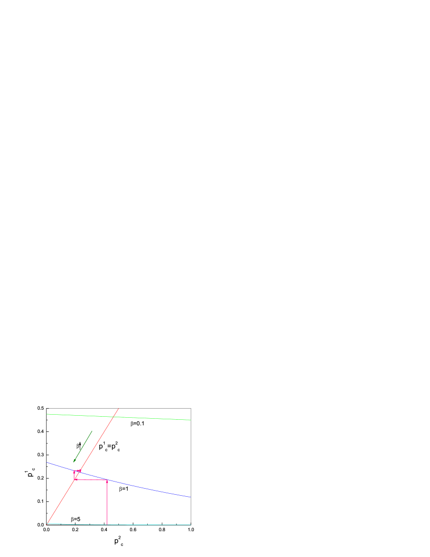
Figure 1: The evolutionary procedure applied onto a classical game with single NE, Prisoner’s Dilemma. The iteration process defined by equ(56) with different value of parameter $\beta$, ends up at one fixed point, which decreases from a finite number to 0 when $\beta$ grows. The meaning of parameter $\beta$ is a measurement of rationality of players[11], and $\beta=\infty$ corresponds to full rational, the case assumed in NE. The solution $0,0$ means both player choose the second strategy and get $-4,-4$ respectively at the end. This gives the same NE as in Classical Game Theory.

5.2 NEs of SRG

In this section, we will discuss the non-cooperative Nash Equilibria of the Spin Rotating Game, defined in equ(31) with payoff Hamiltonian equ(32). According to the restriction discussed in $\S$4.3, basis $\left\{I,iX,iY,iZ\right\}$ is better to be used here. The payoff Hamiltonian will transform consistently. Density matrix of single player state is describe $9$ real numbers, so the strategy state of the two players is

$$\rho^{q,S}=\left[\begin{array}[]{llll}p^{1}_{11}&\alpha^{1}&\beta^{1}&\gamma^{1}\\ \alpha^{1}&p^{1}_{22}&\mu^{1}&\nu^{1}\\ \beta^{1}&\mu^{1}&p^{1}_{33}&\delta^{1}\\ \gamma^{1}&\nu^{1}&\delta^{1}&p^{1}_{44}\end{array}\right]\otimes\left[\begin{array}[]{llll}p^{2}_{11}&\alpha^{2}&\beta^{2}&\gamma^{2}\\ \alpha^{2}&p^{2}_{22}&\mu^{2}&\nu^{2}\\ \beta^{2}&\mu^{2}&p^{2}_{33}&\delta^{2}\\ \gamma^{2}&\nu^{2}&\delta^{2}&p^{2}_{44}\end{array}\right],$$ (60)

with the constrain $p^{1,2}_{11}+p^{1,2}_{22}+p^{1,2}_{33}+p^{1,2}_{44}=1$. Then the payoff is a function of this $18$ real variables,

$$\begin{array}[]{lll}E^{1}=&\begin{array}[]{l}1-2p^{1}_{22}-2p^{1}_{33}-2p^{2}_{22}-2p^{2}_{33}\\ +4p^{1}_{22}p^{2}_{22}+4p^{1}_{22}p^{2}_{33}+4p^{1}_{33}p^{2}_{22}+4p^{1}_{33}p^{2}_{33}\\ -4\alpha^{1}\alpha^{2}-4\beta^{1}\beta^{2}+4\nu^{1}\nu^{2}+4\delta^{1}\delta^{2}\\ +4\alpha^{1}\delta^{2}-4\delta^{1}\alpha^{2}+4\nu^{1}\beta^{2}-4\beta^{1}\nu^{2}\end{array}&=-E^{2}.\end{array}$$ (61)

Next step, we need to solve all NEs from these two functions. One way to find some, but not all, of them is to solve the equations, $\frac{\partial}{\partial x^{2}}E^{1}=0=\frac{\partial}{\partial x^{1}}E^{2}$. Here we still don’t have the general algorithm for quantum game, so in order to demonstrate how our general representation can be used to discuss quantum game in some practical senses, we just use this trivial way to get some NEs. The equations gives condition on the possible value of all $18$ variables as following,

$$\left\{\begin{array}[]{l}p^{1}_{22}+p^{1}_{33}=\frac{1}{2}=p^{2}_{22}+p^{2}_{33}\\ \alpha^{1}+\delta^{1}=0=\alpha^{2}-\delta^{2}\\ \beta^{1}-\nu^{1}=0=\beta^{2}+\nu^{2}\end{array}\right.$$ (62)

Therefore, the NE strategy states could be

$$\rho^{q,S}=\left[\begin{array}[]{llll}p^{1}_{a}&\alpha^{1}&\beta^{1}&\gamma^{1}\\ \alpha^{1}&p^{1}_{b}&\mu^{1}&\beta^{1}\\ \beta^{1}&\mu^{1}&\frac{1}{2}-p^{1}_{b}&-\alpha^{1}\\ \gamma^{1}&\beta^{1}&-\alpha^{1}&\frac{1}{2}-p^{1}_{a}\end{array}\right]\otimes\left[\begin{array}[]{llll}p^{2}_{a}&\alpha^{2}&\beta^{2}&\gamma^{2}\\ \alpha^{2}&p^{2}_{b}&\mu^{2}&-\beta^{2}\\ \beta^{2}&\mu^{2}&\frac{1}{2}-p^{2}_{b}&\alpha^{2}\\ \gamma^{2}&-\beta^{2}&\alpha^{2}&\frac{1}{2}-p^{2}_{a}\end{array}\right].$$ (63)

For example, the classical sub-game with an NE $p^{1}_{a}=\frac{1}{2}=p^{2}_{a}$, is covered by this general NE of quantum game. The intuitive meaning of this general NE can be revealed partially by a special case such as $p^{1}_{a}=\frac{1}{4}=p^{1}_{b},\alpha^{1}\in\left[0,\frac{1}{4}\right]$, which gives the strategies as following,

$$\left\{\begin{array}[]{ll}s^{1}_{1}=\frac{-I+iX}{\sqrt{2}};&p^{1}_{1}=-\alpha^{1}+\frac{1}{4}\\ s^{1}_{2}=\frac{iY+iZ}{\sqrt{2}};&p^{1}_{2}=-\alpha^{1}+\frac{1}{4}\\ s^{1}_{3}=\frac{I+iX}{\sqrt{2}};&p^{1}_{3}=\alpha^{1}+\frac{1}{4}\\ s^{1}_{4}=\frac{iY-iZ}{\sqrt{2}};&p^{1}_{4}=\alpha^{1}+\frac{1}{4}\end{array}\right..$$ (64)

This means a combination of this four pure strategies can act as the mixture strategy of player $1$ in the equilibria.

Works towards an algorithm for the complete NEs and for general games is still in progress. However, by this example, we have shown that our general formalism for sure can be used to describe the general quantum game. And only finite real variables are required, not like the situation in TQG, where infinite number of parameters are needed for general mixture strategy NEs.

5.3 From Quantum Game to Classical Game

A sub-game of this quantum SRG can be defined as the game restricted only in pure and mixture combination of strategies $I,iX$. One may guess that this sub-game will be like the classical PFG, so the payoff matrix should like equ(29). However, the corresponding sub-matrix, in fact, is

$$H_{sub}^{1,2}=\left[\begin{array}[]{llll}1,-1&0&0&1,-1\\ 0&-1,1&-1,1&0\\ 0&-1,1&-1,1&0\\ 1,-1&0&0&1,-1\end{array}\right].$$ (65)

Only the diagonal terms agree with the payoff matrix in equ(29), but it also has more non-zero off-diagonal terms. This raises a question on the condition when a quantum game, or a general game given in the manipulative definition as in equ(3), becomes a classical game.

The first case is when only the diagonal part of payoff matrix is chosen as the payoff matrix of a classical game. This situation happens when we restrict the strategy density matrix only as probability combination of some fixed and given pure strategies. In fact, the relation between above sub-game and PFG is such a case. Under such situation, the set of pure strategies has to be a priori given.

The second case is when a special basis can be found, that under this basis both all $\rho^{i}$ and all $H^{i}$ are diagonal. This requires two facts, first, all payoff matrix commutate with each other,

$$\left[H^{i},H^{j}\right]=0,\forall i,j;$$ (66)

second, the common eigenstates are in the direct-product form, not entangled,

$$\left|E_{m}\right>=\left|E^{1}_{m}\right>\left|E^{2}_{m}\right>.$$ (67)

We have an example of the first case, as SRG and PFG. However, usually, we don’t have an concrete example where the requirement in the second case is fulfilled. For SRG, although $\left[H^{1},H^{2}\right]=0$, the common eigenstates are entangled. The two requirement in the second case will be fulfilled if the payoff matrices are in the direct-product form: $H^{i}=h^{i,1}\otimes h^{i,2}$ and $\left[h^{i,m},h^{j,m}\right]=0$. But we don’t know if there is a real game existing in such a form. Therefore, we’d better adopt the first case as the way from quantum game to classical game: only the probability combination of given pure strategies can act as strategy in the game so that only the diagonal part of payoff matrix is effective.

6 Remarks

Both Classical Game and Quantum Game, both non-cooperative game and coalitional game, can be generally unified in the new representation, the operator representation, or the Hamiltonian Formalism. We have shown that the new quantum game defined in this new representation is different with the Traditional Quantum Game, and is not in the scope of Classical Game Theory, which usually uses the probability distribution over the set of pure strategies as strategy state. And the entanglement of strategy is not the usual meaning of entanglement of object state.

The classical game and the TQG are just the same thing, except in the latter, a lager strategy space has to be used. That’s the reason of the conclusion in [10] and [7], it was claimed that, there is no independent meaning of quantum game, only possibly with different efficiency. However, our quantum game is different with TQG. The probability distribution is replaced by a density matrix. And this replacement is significantly different. So, if we compare the classical game with our new quantum game, the difference is: both $\rho^{C}$ and $H^{i,C}$, state and payoff matrixes of classical players are diagonal matrix, while the ones of quantum player $\rho^{Q}$ and $H^{i,Q}$ generally have off-diagonal elements. This is similar to the difference between classical system and quantum system. Therefore, our new quantum game has independent meaning other than the classical game, just like the relation between Classical Mechanics and Quantum Mechanics, but under the same spirit of Game Theory. By replacing the TQG with our new quantum game, the spirit of Game Theory is reserved while the scope of game theory is extended. So we are not arguing that the TQG is independent of classical game, but our new quantum game is. The operators $H$ used in abstract definition looks similar with the matrix form used in [7], however, with different meanings. In our notation, $H$ are operators which give payoff when acting on state of density matrix, while in [7] they does not have the meaning of an operator over a Hilbert space, and the state of players there is still a probability distribution.

It’s argued in section $\S$5.3, principally and by one example, lower work load need to be done to search for the NEs in our representation than in the traditional quantum game. However, neither the existence of the general/special NEs been proved here, nor an applicable algorithm to find them has been discovered. The relation between our general NEs and Coalitional game has been reached by examples in [14], but not treated generally and theoretically.

Another thing need to be mentioned is the necessity to introduce the manipulative definition. At one hand, in fact, it’s not necessary. Here, it’s introduced to be a bridge between classical and quantum game. From the manipulative definition, it’s easy to know the quantum games are just games on quantum objects while classical games are games on classical objects. At the other hand, it’s valuable. Readers from Classical Game Theory usually work on games directly at the abstract definition. But we believe that every classical game can be mapped onto a manipulative definition, although probably not unique. For example, one can always check the background where the game comes from. Whenever we have the manipulative definition, quantization of such game will be easy.

7 Acknowledgement

Thanks Dr. Shouyong Pei for the stimulating discussion during every step of progress of this work. Thanks Dr. Qiang Yuan, Dr. Zengru Di and Dr. Yougui Wang for their help on the entrance of Game Theory, their great patience to discuss with me when the idea of this paper is so ambiguous and rough and also for their invitation so that I can get the chance to give a talk and discuss with more people on this. Thanks should also be given to Prof. Zhanru Yang and Dr. Bo Chen for their reading and comments, and Dr. Jens Eisert for his encouragement. Thanks Taksu Cheon for the discussion on the mapping between strategy vector and density matrix.

References

- [1] Morikazu Toda, M. Toda, N. Saito, R. Kubo, Ryogo Kubo, and N. Hsshitsume, Statistical Physics II: Nonequilibrium Statistical Mechanics (2ND Edition, Springer Series in Solid-State Sciences, 1991).
- [2] M.E.J. Newman and G.T. Barkema, Monte Carlo Method in Statistical Physics (New York: Oxford University Press, 1999).
- [3] M. J. Osborne and A. Rubinstein, A course in Game Theory (MIT Press, 1994).
- [4] M.A. Nielsen and I.L. Chuang, Quantum Computation and Quantum Information (Cambridge Univ. Press, 2000), page 20, in Box1.1.
- [5] D.A. Meyer, Phys. Rev. Lett. 82(1999), 1052.
- [6] J. Eisert, M. Wilkens, and M. Lewenstein, Phys. Rev. Lett, 83(1999), 3077.
- [7] C.F. Lee and N.F. Johnson, Phys. Rev. A 67(2003), 022311.
- [8] S.C. Benjamin and P.M. Hayden, Phys. Rev. A, 64(2001), 030301.
- [9] L. Marinatto and T. Weber, Phys. Lett. A 272(2000), 291.
- [10] S. J. van Enk and R. Pike, Phys. Rev. A 66(2002), 024306.
- [11] D.H. Wolpert, arXiv:cond-mat/0402508.
- [12] J. Wu, arXiv:quant-ph/0404159.
- [13] J. Wu, arXiv:quant-ph/0405183.
- [14] J. Wu, arXiv:quant-ph/0405003.