Entanglement in spin-one Heisenberg chains

Abstract

By using the concept of negativity, we study entanglement in spin-one Heisenberg chains. Both the bilinear chain and the bilinear-biquadratic chain are considered. Due to the SU(2) symmetry, the negativity can be determined by two correlators, which greatly facilitate the study of entanglement properties. Analytical results of negativity are obtained in the bilinear model up to four spins and the two-spin bilinear-biquadratic model, and numerical results of negativity are presented. We determine the threshold temperature before which the thermal state is doomed to be entangled.

I Introduction

Since Haldane predicts that the one-dimensional Heisenberg chain has a spin gap for integer spins Haldane , the physics of quantum spin chains has been the subject of many theoretical and experimental studies. In these studies, the bilinear spin-one Heisenberg model and the bilinear-biquadratic Heisenberg model have played important roles Affleck ; Millet ; Xiang . The corresponding Hamiltonians are given by

$$H_{1}= \sum_{i=1}^{N}J{\bf S}_{i}\cdot{\bf S}_{i+1},$$ (1)

$$H_{2}= \sum_{i=1}^{N}\left[J{\bf S}_{i}\cdot{\bf S}_{i+1}+\gamma({\bf S}_{i}\cdot{\bf S}_{i+1})^{2}\right],$$ (2)

respectively. Here, we have assumed the periodic boundary condition, and obviously, these two Hamiltonians exhibits a SU(2) symmetry. Moreover, the bilinear-biquadratic model exhibits very rich phase diagram Schollwock .

Recently, the study of entanglement properties in Heisenberg systems have received much attention M_Nielsen -QPT_GVidal . Quantum entanglement lies at the heart of quantum mechanics, and can be exploited to accomplish some physical tasks such as quantum teleportation Tele . Spin-half systems have been considered in most of these studies. However, due to the lack of entanglement measure for higher spin systems, the entanglement in higher spin systems have been less studied. There are several proceeding works on entanglement in spin-one chains. Fan et al. Fan and Verstraete et al. Verstraete studied entanglement in the bilinear-biquadratic model with a special value of $\gamma=1/3$, i.e., the AKLT model Affleck . Zhou et al. studied entanglement in the Hamiltonian $H_{2}$ for the case of two spins Zhou .

In this paper, by using the concept of negativity Vidal , we study pairwise entanglement in both the bilinear and the bilinear-biquadratic Heisenberg spin-one models. For the case of higher spins, a non-entangled state has necessarily a positive partial transpose (PPT) according to the Peres-Horodecki criterion PH . In the case of two spin halves, and the case of (1/2,1) mixed spins, a PPT is also sufficient. However, in the case of two spin-one particles, a PPT is not sufficient. Nevertheless, the negative partial transpose (NPT) gives a sufficient condition for entanglement, and due to the SU(2) symmetry in the systems, the NPT is expected to fully capture the entanglement properties.

The Peres-Horodecki criterion give a qualitative way for judging if the state is entangled. The quantitative version of the criterion was developed by Vidal and Werner Vidal . They presented a measure of entanglement called negativity that can be computed efficiently, and the negativity does not increase under local manupulations of the system. The negativity of a state $\rho$ is defined as

$${\cal N(\rho)}=\sum_{i}|\mu_{i}|,$$ (3)

where $\mu_{i}$ is the negative eigenvalue of $\rho^{T_{2}}$, and $T_{2}$ denotes
the partial transpose with respect to the second system. The negativity ${\cal N}$ is related to the trace norm of $\rho^{T_{2}}$ via

$${\cal N(\rho)}=\frac{\|\rho^{T_{2}}\|_{1}-1}{2},$$ (4)

where the trace norm of $\rho^{T_{2}}$ is equal to the sum of the absolute values of the eigenvalues of $\rho^{T_{2}}$. If ${\cal N}>0$, then the two-spin state is entangled.

We study entanglement in both the ground state and the thermal state. The state of a system at thermal equilibrium described by the density operator $\rho(T)=\exp(-\beta H)/Z$, where $\beta=1/k_{B}T$, $k_{B}$ is the Boltzmann’s constant, which is assume to be 1 throughout the paper , and $Z=\text{Tr}\{\exp(-\beta H)\}$ is the partition function. The entanglement in the thermal state is called thermal entanglement.

We organize the paper as follows. In Sec. II, we give the exact forms of the negativity for an SU(2)-invariant state, and show how the negativity is related to two correlators. We also give that how to obtain negativity from the ground-state energy and partition function in the bilinear-biquadratic model. We study entanglement in the bilinear and bilinear-biquadratic models in Sec. III and IV, respectively. Some analytical and numerical results of negativity are obtained. We conclude in Sec. V.

II Negativity and correlators

Schliemann considered the entanglement of two spin-one particles via the Peres-Horodecki criteria Schliemann , and find that the SU(2)-invariant two-spin state is entangled if either of the following inequalities holds

$$\langle({\bf S}_{i}\cdot{\bf S}_{j})^{2}\rangle>2,$$

$$\langle({\bf S}_{i}\cdot{\bf S}_{j})^{2}\rangle+\langle{\bf S}_{i}\cdot{\bf S}_{j}\rangle<1.$$ (5)

Now we explicitly give the expression of negativity for the SU(2)-invariant two-spin state.

According to the SU(2)-invariant symmetry, any state of two spin-one particles have the general form Schliemann

$$\rho= G|S=0,S_{z}=0\rangle\langle S=0,S_{z}=0|$$

$$+\frac{H}{3}\sum_{S_{z}=-1}^{1}|S=1,S_{z}\rangle\langle S=1,S_{z}|$$

$$+\frac{1-G-H}{5}\sum_{Sz=-2}^{2}|S=2,S_{z}\rangle\langle S=2,S_{z}|,$$ (6)

where $|S,S_{z}\rangle$ denotes a state of total spin $S$ and $z$ component $S_{z}$, and

$$G= \frac{1}{3}[\langle({\bf S}_{i}\cdot{\bf S}_{j})^{2}\rangle-1],$$

$$H= 1-\frac{1}{2}[\langle{\bf S}_{i}\cdot{\bf S}_{j}\rangle+\langle({\bf S}_{i}\cdot{\bf S}_{j})^{2}\rangle].$$ (7)

In order to perform partial transpose, the product basis spanned by $\{|S_{1}=1,S_{1z}\rangle\otimes|S_{2}=1,S_{2z}\rangle\}$ is a natural choice. By using the Clebsch-Gordan coefficients, we may write state $\rho$ in the product basis. The partially transposed with respect to the second spin $\rho^{T_{2}}$ can be written in a block-diagonal form with two $1\times 1$ block, two $2\times 2$ block, and one $3\times 3$ block. After diagonalization of each block, one find that the following only two eigenvalues of $\rho^{T_{2}}$ are possibly negative Schliemann ,

$$\mu_{1}= \frac{1}{6}(2-\langle({\bf S}_{i}\cdot{\bf S}_{j})^{2}\rangle),$$

$$\mu_{2}= \frac{1}{3}(\langle{\bf S}_{i}\cdot{\bf S}_{j}\rangle+\langle({\bf S}_{i}\cdot{\bf S}_{j})^{2}\rangle-1).$$ (8)

Moreover, $\mu_{1}$ and $\mu_{2}$ occur with multiplicities 3 and 1, respectively. Therefore, the negativity is obtained as

$${\cal N}^{(ij)}= \frac{1}{2}\max[0,\langle({\bf S}_{i}\cdot{\bf S}_{j})^{2}\rangle-2]$$

$$+ \frac{1}{3}\max[0,1-\langle({\bf S}_{i}\cdot{\bf S}_{j})\rangle-\langle({\bf S}_{i}\cdot{\bf S}_{j})^{2}\rangle].$$ (9)

We see that for the SU(2)-invariant state, the negativity is completely determined by two correlators $\langle({\bf S}_{i}\cdot{\bf S}_{j})\rangle$ and $\langle({\bf S}_{i}\cdot{\bf S}_{j})^{2}\rangle$.

Recall that the swap operator between two spin-one particles is given by

$${\cal S}_{ij}={\bf S}_{i}\cdot{\bf S}_{j}+({\bf S}_{i}\cdot{\bf S}_{j})^{2}-I$$ (10)

where $I$ denotes the $9\times 9$ identity matrix. Then, the negativity can be written in the following form

$${\cal N}^{(ij)}= \frac{1}{2}\max[0,\langle{\cal S}_{ij}\rangle-\langle{\bf S}_{i}\cdot{\bf S}_{j}\rangle-1]$$

$$+ \frac{1}{3}\max[0,-\langle{\cal S}_{ij}\rangle].$$ (11)

We see that if the expectation value $\langle{\cal S}_{ij}\rangle<0$, the state is entangled. The swap operator satisfies ${\cal S}_{ij}=1$, and thus it has only two eigenvalues $\pm 1$. If a state is a eigenstate of the swap operator, the expression (II) can be simplified. When the corresponding eigenvalue is 1, Equation (II) simplifies to

$${\cal N}^{(ij)}=\frac{1}{2}\max[0,-\langle{\bf S}_{i}\cdot{\bf S}_{j}\rangle],$$ (12)

and when the eigenvalue is -1, the equation simplifies to

$${\cal N}^{(ij)}=\frac{1}{3}+\frac{1}{2}\max[0,-\langle{\bf S}_{i}\cdot{\bf S}_{j}\rangle-2].$$ (13)

In the former case, the state is entangled if $\langle{\bf S}_{i}\cdot{\bf S}_{j}\rangle<0$, and in the latter case, the state is an entangled state, and the negativity is larger than or equal to 1/3.

Now we consider the bilinear-biquadratic spin-one Heisenberg model described by the Hamiltonian $H_{2}$. By applying the Hellmann-Feynman theorem to the ground state of $H_{2}$ and considering the translational invariance, we may obtain the correlators as

$$\langle({\bf S}_{i}\cdot{\bf S}_{i+1})\rangle=\frac{1}{N}\frac{\partial E_{\text{GS}}}{\partial J},\;\langle({\bf S}_{i}\cdot{\bf S}_{i+1})^{2}\rangle=\frac{1}{N}\frac{\partial E_{\text{GS}}}{\partial\gamma},$$ (14)

where $E_{\text{GS}}$ is the ground-state energy. Substituting the above equation into Eq. (II) yields

$${\cal N}^{(ii+1)}= \frac{1}{2}\max\Big{[}0,\frac{1}{N}\frac{\partial E_{\text{GS}}}{\partial\gamma}-2\Big{]}$$

$$+ \frac{1}{3}\max\Big{[}0,1-\frac{1}{N}\frac{\partial E_{\text{GS}}}{\partial J}-\frac{1}{N}\frac{\partial E_{\text{GS}}}{\partial\gamma}\Big{]}.$$ (15)

For the case of finite temperature, we have

$${\cal N}^{(ii+1)}= \frac{1}{2}\max\Big{[}0,\frac{-1}{N\beta Z}\frac{\partial Z}{\partial\gamma}-2\Big{]}$$

$$+ \frac{1}{3}\max\Big{[}0,1+\frac{1}{N\beta Z}\frac{\partial Z}{\partial J}+\frac{1}{N\beta Z}\frac{\partial Z}{\partial\gamma}\Big{]}.$$ (16)

We see that the knowledge of ground-state energy (partition function) is sufficient to determine the negativity for the case of zero temperature (finite temperature).

III Bilinear Heisenberg model

Let us know consider the entanglement in the bilinear Heisenberg model. Due to the nearest-neighbor character of the interaction, the entanglement between two nearest-neighbor spins is prominent compared with two non-nearest-neighbor spins. Thus, we focus on the nearest-neighbor case in the following discussions of entanglement.

III.1 Two spins

For systems with a few spin, we aim at obtaining analytical results of negativity. The Hamiltonian for two spins can be written as

$$H_{1}={\bf S}_{1}\cdot{\bf S}_{2}=\frac{1}{2}[({\bf S}_{1}+{\bf S}_{2})^{2}-{\bf S}_{1}^{2}-{\bf S}_{2}^{2}],$$ (17)

from which all the eigenvalues of the system are given by

$$E_{0}=-2(1),\;E_{1}=-1(3),\;E_{2}=1(5),$$ (18)

where the number in the bracket denotes the degeneracy.

We investigate the entanglement of all eigenstates of the system. When an energy level of our system is non-degenerate, the corresponding eigenstate is pure. When a $k$-th energy level is degenerate, we assume that the corresponding state is an equal mixture of all eigenstates with energy ${\cal E}_{k}$. Thus, the state correspoding to the $k$-th level with degeneracy becomes a mixed other than pure, keeping all symmetries of the Hamiltonian. A degenerate ground state is called thermal ground state in the sense that it can be obtained from the thermal state $\exp[-H/(k_{B}T)]/Z$ by taking the zero-temperature limit M_Osborne . The $k$-th eigenstate $\rho_{k}$ can be considered as the thermal ground state of the nonlinear Hamiltonian $H^{\prime}$ given by $H^{\prime}=(H-{E}_{k})^{2}$. Note that Hamiltonian $H^{\prime}$ inherits all symmetries of Hamiltonian $H$.

As we consider interaction of two spins, from Eqs. (17) and (II), we obtain another form of the negativity as

$${\cal N}^{(12)}= \frac{1}{2}\max[0,\langle H^{2}_{1}\rangle-2]$$

$$+\frac{1}{3}\max[0,1-\langle H_{1}+H^{2}_{1}\rangle].$$ (19)

To determine the negativity, it is sufficient to know the cumulants $\langle H_{1}\rangle$ and $\langle H_{1}^{2}\rangle$.

From Eqs. (III.1) and (18), the negativities correspond to the $k$-th level are obtained as

$${\cal N}_{0}^{(12)}=1,\;{\cal N}_{1}^{(12)}=1/3,\;{\cal N}_{2}^{(12)}=0.$$ (20)

We see that the ground state is a maximally entangled state, the first-excited state is also entangled, but the negativity of the second-excited state is zero.

Having known negativities of all eigenstates, we next consider the case of finite temperature. The cumulants can be obtained from the partition function. From Eq. (18), the partition function is given by

$$Z=e^{2\beta}+3e^{\beta}+5e^{-\beta}.$$ (21)

A cumulant of arbitrary order can be calculated from the partition function,

$$\langle H_{1}^{n}\rangle= \frac{(-1)^{n}}{Z}\frac{\partial^{n}}{\partial\beta^{n}}Z$$

$$= \frac{(-1)^{n}}{Z}\left[2^{n}e^{2\beta}+3e^{\beta}+5(-1)^{n}e^{-\beta}\right]$$ (22)

Substituting the cumulants with $n=1,2$ to Eq. (III.1) yields

$${\cal N}= \frac{1}{2Z}\max\left(0,2e^{2\beta}-3e^{\beta}-5e^{-\beta}\right)$$

$$+\frac{1}{3Z}\max\left(0,3e^{\beta}-e^{2\beta}-5e^{-\beta}\right).$$ (23)

Thus, we obtain the analytical expression of the negativity.

The second term in Eq. (III.1) can be shown to be zero. To see this fact, it is sufficient to show that $F(x)=x^{3}-3x^{2}+5>0$, where $x=e^{\beta}>1$. It is direct to check that the function $F$ takes its minimum 1 at $x=2$. As the minimum is large than zero, the function is positive definite. Thus, equation (III.1) simplifies to

$${\cal N}=\frac{1}{2Z}\max\left(0,2e^{2\beta}-3e^{\beta}-5e^{-\beta}\right).$$ (24)

The behavior of the negativity versus temperature is similar to that of the concurrence Conc in the spin-half Heisenberg model M_Arnesen , namely, the negativity decreases as the temperature increases, and there exists a threshold value of temperature $T_{\text{th}}$, after which the negativity vanished. This behavior is easy to understand as the increase of temperature leads to the increase of probability of the excited states in the the thermal state, and the excited states are less entangled in comparison with the ground state. From Eq. (24), the threshold temperature can be analytically obtained as

$$T_{\text{th}}= \frac{1}{\ln(\frac{1}{2}+\frac{1}{2(11+2\sqrt{30})^{1/3}}+\frac{(11+2\sqrt{30})^{1/3}}{2})}$$

$$\approx 1.3667.$$ (25)

III.2 Three spins

The Hamiltonian for three spins is rewritten as

$$H_{1}=\frac{1}{2}[({\bf S}_{1}+{\bf S}_{2}+{\bf S}_{3})^{2}-{\bf S}_{1}^{2}-{\bf S}_{2}^{2}-{\bf S}_{3}^{2}],$$ (26)

from which the ground-state energy and the correlator $\langle{\bf S}_{1}\cdot{\bf S}_{2}\rangle$ are immediately obtained as

$$E_{\text{GS}}=-3,\;\langle{\bf S}_{1}\cdot{\bf S}_{2}\rangle=-1.$$ (27)

In order to know the ground-state negativity, we need to calculator another correlator $\langle({\bf S}_{1}\cdot{\bf S}_{2})^{2}\rangle$.

By considering the translational invariance and using similar techniques given by Refs.Kouzoudis ; Schnack ; Lin , the ground-state vector is obtained as

$$|\Psi\rangle_{\text{GS}}=\frac{1}{\sqrt{6}}( |012\rangle+|201\rangle+|120\rangle$$

$$- |021\rangle-|102\rangle-|210\rangle),$$ (28)

where $|n\rangle$ denote the state $|s=1,m=s-n\rangle$, the common eigenstate of ${\bf S}^{2}$ and $S_{z}$. Then, we can check that

$${\bf S}_{1}\cdot{\bf S}_{2}|\Psi\rangle_{\text{GS}}=-|\Psi\rangle_{\text{GS}}.$$ (29)

Thus, the correlator $\langle({\bf S}_{1}\cdot{\bf S}_{2})^{2}\rangle$ is found to be

$$\langle({\bf S}_{1}\cdot{\bf S}_{2})^{2}\rangle=1.$$ (30)

Substituting Eqs. (27) and (30) to Eq. (II) yields

$${\cal N}=1/3.$$ (31)

We see that spins 1 and 2 are in an entangled state at zero temperature. With the increase of temperature, the negativity monotonically decreases until it reaches the threshold value $T_{\text{th}}=0.9085$, after which the negativity vanishes.

III.3 Four spins

Now we consider the four-spin case, and the corresponding Hamiltonian can be written as

$$H_{1}=\frac{1}{2}[({\bf S}_{1}+{\bf S}_{2}+{\bf S}_{3}+{\bf S}_{4})^{2}-({\bf S}_{1}+{\bf S}_{3})^{2}-({\bf S}_{2}+{\bf S}_{4})^{2}].$$ (32)

The standard angular momentum coupling theory directly yields the ground-state energy and the correlator $\langle{\bf S}_{1}\cdot{\bf S}_{2}\rangle$

$$E_{\text{GS}}=-6,\;\langle{\bf S}_{1}\cdot{\bf S}_{2}\rangle=-3/2.$$ (33)

Then, we need to compute another correlator $\langle({\bf S}_{1}\cdot{\bf S}_{2})^{2}\rangle$ or alternatively the expectation value $\langle{\cal S}_{12}\rangle$. So, it is necessary to know the exact form of the ground state.

By using similar techniques given by Refs.Kouzoudis ; Schnack ; Lin , the ground-state vector is obtained as

$$|\Psi\rangle_{\text{GS}}= 1/2|\psi_{1}\rangle-3/2|\psi_{2}\rangle+|\psi_{3}\rangle$$

$$-3/2|\psi_{4}\rangle+3/\sqrt{2}|\psi_{5}\rangle+|\psi_{6}\rangle.$$ (34)

where

$$|\psi_{1}\rangle= 1/2(|0022\rangle+|2002\rangle+|2200\rangle+|0220\rangle),$$

$$|\psi_{2}\rangle= 1/2(|0112\rangle+|2011\rangle+|1201\rangle+|1120\rangle),$$

$$|\psi_{3}\rangle= 1/2(|0121\rangle+|1012\rangle+|2101\rangle+|1210\rangle),$$

$$|\psi_{4}\rangle= 1/2(|0211\rangle+|1021\rangle+|1102\rangle+|2110\rangle),$$

$$|\psi_{5}\rangle= 1/\sqrt{2}(|0202\rangle+|2020\rangle),$$

$$|\psi_{6}\rangle= |1111\rangle.$$ (35)

Then, from the explicit form of the ground state, after two-page calculations, we obtain the expectation value of the swap operator as

$$\langle{\cal S}_{12}\rangle=1/6.$$ (36)

Substituting Eqs. (33) and (36) to Eq. (II) leads to

$${\cal N}=1/3.$$ (37)

It is interesting to see that the ground-state negativity in the four-qubit model is the same as that in the three-qubit model. The threshold value can be found to be $T_{\text{th}}=1.3804$.

For $N\geq 5$, it is hard to obtain analytical results of negativity. The behaviors of negativity are similar to those for $N\leq 4$, namely, with the increase of temperature, the negativity decreases until it vanishes at threshold temperature $T_{\text{th}}$. For instance, the threshold temperatures $T_{\text{th}}\approx 0.95$ and $T_{\text{th}}\approx 1.21$ for five and six spins, respectively. The negativity for two nearest-neighbors spins is estimated as ${\cal N}=0.1240$ (${\cal N}=0.2509$) for the case of five spins (six spins).

IV Bilinear-Biquadratic Spin-One Heisenberg Chain

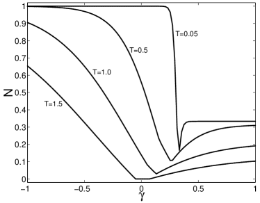
Figure 1: Negativity versus $\gamma$ for different temperatures in the two-spin model ($J=1$).

We now study entanglement properties in the bilinear-biquadratic spin-one Heisenberg model, and first consider the case of two spins. From Eq. (II) with $N=1$, if we know the ground-state energy, the negativity is readily obtained. The ground-state energy is given by

$$E_{\text{GS}}=\left\{\begin{array}[]{ll}-2J+4\gamma&\;\text{when}\;\gamma<1/3,\\ -1J+\gamma&\;\text{when}\;\gamma>1/3,\end{array}\right.$$ (38)

We see that there exits a level crossing at the point of $\gamma=1/3$. Then, substituting the above equation into Eq. (II) yields

$${\cal N}=\left\{\begin{array}[]{ll}1&\;\text{when}\;\gamma<1/3,\\ 1/3&\;\text{when}\;\gamma>1/3,\end{array}\right.$$ (39)

Before the point $\gamma=1/3$, the negativity of the ground-state is 1, while the negativity of the first-excited state is 1/3. After the cross point, the ground and first-excited interchanges, and thus, the negativity of the ground state after the cross point is 1/3. It is interesting to see that the model at the cross point is just the AKLT model.

In Fig. 1, we plot the negativity versus $\gamma$ for different temperatures. The level cross greatly affects the behaviors of the negativity at finite temperatures. For a small temperature ($T=0.05$), the negativity displays a jump from 1 to 1/3 near the cross point. For higher temperatures, the negativity first decreases, and then increases at $\gamma$ increases from -1 to 1. For $T=1.5$, we observe that there exists a range of $\gamma$, in which the negativity is zero.

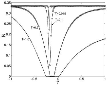
Figure 2: Negativity versus $\gamma$ for different temperatures in the three-spin model ($J=1$).

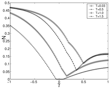
Figure 3: Negativity versus $\gamma$ for different temperatures in the four-spin model ($J=1$).

For the three-spin case, we plot the negativity versus $\gamma$ for different temperatures in Fig. 2. For a low temperature $T=0.015$, we observe a dip, which results from the level crossing near the point of $\gamma=-0.2121$. When $T=0.1$, the dip becomes more evident. For the cases of higher temperatures ($T=0.5$ and $T=1.0$), there exists a range of parameter $\gamma$, in which the negativity is zero.

For the four-spin case, we also a plot of the negativity for different temperatures. For $T=0.03$, as $\gamma$ increases, the negativity decreases until it reaches its minimum, and then increases. For $T=0.5$ and $1.0$, the behaviors of negativity are similar to the case of $T=0.01$, and the difference is that the minima shifts left. There are some common features in the behaviors of negativity for different number of spins. The maximum value of negativity occurs at $\gamma=-1$; for higher temperatures, there exists a range of $\gamma$, in which the negativity is zero.

From Figs. 1-3, we observe that the thermal state is always entangled at a lower temperature. When temperature increases, the negativity decreases until it reaches zero, namely, the thermal fluctuation suppresses entanglement. Before the threshold temperature, the state is doomed to be entangled. We numerically calculated the threshold temperature and the result are shown in Fig. 4. The threshold temperature decreases nearly linearly when $\gamma$ increases from -1 to a certain value of $\gamma$. After reaching a minimum, it begin to increase. We see that the behaviors of the threshold temperature are similar for different number of spins.

As a final remark, we consider the following Hamiltonian

$$H_{3}=\sum_{i\neq j}^{N}J{\bf S}_{i}\cdot{\bf S}_{j}=\frac{1}{2}\left(\sum_{i=1}^{N}{\bf S}_{i}\right)^{2}-N,$$ (40)

where the interaction is between all spins, and there are all together $N(N-1)/2$ terms. The system not only shows a SU(2) symmetry, but also an exchange symmetry, namely, the Hamiltonian in invariant under exchange operation ${\cal S}_{ij}H_{3}{\cal S}_{ij}=H_{3}$. For $N=2,3$, the model is identical to Hamiltonian $H_{2}$. We know that the ground state is non-degenerate when $N=2,3$, and thus it must be an eigenstate of $S_{ij}$ and Eqs. (12) and (13) can apply. From the angular momentum coupling theory, the ground-state energy of $H_{3}$ is readily obtained as $E_{\text{GS}}=-N$, and thus we have $\langle{\bf S}_{i}\cdot{\bf S}_{j}\rangle=-2/(N-1)$. Then, from Eqs. (12) and (13), the negativity can be either $1/(N-1)$ or $1/3$. For $N=2$ ($N=3$), the ground state is symmetric (antisymmetric) and then the negativity is 1 (1/3), consistent with previous results. However, for $N\geq 4$, the ground-state is degenerate and we cannot apply Eqs. (12) and (13). The numerical results show that the negativity is zero for $N\geq 4$.

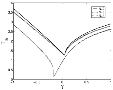
Figure 4: Threshold temperature versus $\gamma$ for different number of spins.

V Conclusions

In conclusion, by using the concept of negativity, we have studied entanglement in spin-one Heisenberg chains. Both the bilinear model and bilinear-biquadratic model are considered. Although NPT only give a sufficient condition for entanglement, due to the SU(2) symmetry, we believe that this condition considerably captures entanglement properties of the system. Moreover, the negativity gives an upper bound to the distillation of entanglement Vidal , one of the fundamental entanglement measures. We have given explicitly the relation between the negativity and two correlators. The merit of this relation is that the two correlators completely determine the negativity and it facilitates our discussions of entanglement properties.

We have obtained analytical results of negativity in the bilinear model up to four spins and in the two-spin bilinear-biquadratic model. We numerically calculated entanglement in the bilinear-biquadratic model for $N=2,3,4$, and the threshold temperatures versus $\gamma$ are also given. We have restricted us to the small-size systems, and aimed at obtaining analytical results via symmetry considerations and getting some numerical results via the exact diagonalization method. However, for larger systems, the exact diagonalization method is not a viable route. It is interesting to investigate large systems by some mature numerical methods such as the quantum monte-carlo method and density-matrix renomalization group method. And it is also interesting to consider other SU(2)-invariant spin-one systems such as the dimerized and frustrated systems.

- (1) F. D. M. Haldane, Phys. Lett. 93A, 464 (1983); F. D. M. Haldane, Phys. Rev. Lett. 50, 1153 (1983).
- (2) I. Affleck, T. Kennedy, E. H. Lieb, and H. Tasaki, Phys. Rev. Lett. 59, 799 (1987).
- (3) P. Millet, F. Mila, F. C. Zhang, M. Mambrini, A. B. Van Oosten, V. A. Pashchenko, A. Sulpice, and A. Stepanov, Phys. Rev. Lett. 83, 4176 (1999).
- (4) J. Z. Lou, T. Xiang, and Z. B. Su, Phys. Rev. Lett. 85, 2380 (2000).
- (5) Schollwöck, T. Jolicoeur, and T. Garel, Phys. Rev. B53, 3304 (1996).
- (6) M. A. Nielsen, Ph. D thesis, University of Mexico, 1998, quant-ph/0011036;
- (7) M. C. Arnesen, S. Bose, and V. Vedral, Phys. Rev. Lett. 87, 017901 (2001).
- (8) D. Gunlycke, V. M. Kendon, V. Vedral, and S. Bose, Phys. Rev. A64, 042302 (2001).
- (9) X. Wang, Phys. Rev. A 64, 012313 (2001); Phys. Lett. A 281, 101 (2001); X. Wang and P. Zanardi, Phys. Lett. A 301, 1 (2002); X. Wang, Phys. Rev. A 66, 044305 (2002); X. Wang, H. Fu, and A. I. Solomon, J. Phys. A: Math. Gen. 34, 11307(2001); X. Wang and K. Mølmer, Eur. Phys. J. D 18, 385(2002).
- (10) G. Jaeger, A. V. Sergienko, B. E. A. Saleh, and M. C. Teich, Phys. Rev. A68, 022318 (2003).
- (11) S. Bose and V. Vedral, Phys. Rev. A61, 040101 (2000).
- (12) G. L. Kamta and A. F. Starace, Phys. Rev. Lett. 88, 107901 (2002).
- (13) K. M. O’Connor and W. K. Wootters, Phys. Rev. A63, 0520302 (2001).
- (14) D. A. Meyer and N. R. Wallach, quant-ph/0108104.
- (15) T. J. Osborne and M. A. Nielsen, Phys. Rev. A66, 032110 (2002).
- (16) A. Osterloh, L. Amico, G. Falci and R. Fazio, Nature 416, 608 (2002).
- (17) Y. Sun, Y. G. Chen, and H. Chen, Phys. Rev. A 68, 044301 (2003).
- (18) U. Glaser, H. Büttner, and H. Fehske, Phys. Rev. A68, 032318 (2003).
- (19) L. F. Santos, Phys. Rev. A67, 062306 (2003).
- (20) Y. Yeo, Phys. Rev. A66, 062312 (2002).
- (21) D. V. Khveshchenko, Phys. Rev. B68, 193307 (2003).
- (22) L. Zhou, H. S. Song, Y. Q. Guo, and C. Li, Phys. Rev. A68, 024301 (2003).
- (23) G. K. Brennen, S. S. Bullock, Phys. Rev. A70, 52303 (2004).
- (24) R. Xin, Z. Song, and C. P. Sun, quant-ph/0411177.
- (25) G. Tóth, quant-ph/0406061.
- (26) F. Verstraete, M. Popp, and J. I. Cirac, Phys. Rev. Lett. 92, 027901 (2004).
- (27) F. Verstraete, M. A. Martin-Delgado, J. I. Cirac, Phys. Rev. Lett. 92, 087201 (2004).
- (28) J. Vidal, G. Palacios, and R. Mosseri, Phys. Rev. A 69, 022107 (2004).
- (29) N. Lambert, C. Emary, and T. Brandes, Phys. Rev. Lett. 92, 073602 (2004).
- (30) S. Ghose, T. F. Rosenbaum, G. Aeppli, and S. N. Coppersmith, Nature (London) 425, 48 (2003).
- (31) J. Schliemann, Phys. Rev. A68, 012309 (2003).
- (32) C. Brukner, V. Vedral, and A. Zeilinger, quant-ph/0410138; C. Brukner and V. Vedral, quant-ph/0406040.
- (33) H. Fan, V. Korepin, and V. Roychowdhury, Phys. Rev. Lett. 93, 227203 (2004).
- (34) F. Verstraete, M. A. Martín-Delgado, and J. I. Cirac, Phys. Rev. Lett. 92, 087201 (2004).
- (35) L. Zhou, X. X. Yi, H. S. Song, and Y. Q. Quo, quant-ph/0310169.
- (36) S. J. Gu, H. Q. Lin, and Y. Q. Li, Phys. Rev. A68, 042330 (2003).
- (37) X. Wang, Phys. Rev. E 69, 066118 (2004); Phys. Lett. A 329, 439 (2004); Phys. Lett. A, accepted.
- (38) Y. Chen, P. Zanardi, Z. D. Wang, and F. C. Zhang, quant-ph/0407228.
- (39) G. Vidal, J. I. Latorre, E. Rico, and A. Kitaev Phys. Rev. Lett. 90, 227902 (2003).
- (40) C. H. Bennett, G. Brassard, C. Crepeau, R. Jozsa, A. Peres, and W. K. Wootters, Phys. Rev. Lett. 70, 1895 (1993).
- (41) G. Vidal and R. F. Werner, Phys. Rev. A65, 032314 (2002).
- (42) A. Peres, Phys. Rev. Lett. 77, 1413 (1996); M. Horodecki, P. Horodecki, and R. Horodecki, Phys. Lett. A 223, 1 (1996).
- (43) W. K. Wootters, Phys. Rev. Lett. 80, 2245 (1998).
- (44) D. Kouzoudis, J. Magn. Magn. Mater. 173, 259 (1997); ibid 189, 366 (1998).
- (45) K. Bärwinkel, H.-J. Schmidt, and J. Schnack, J. Magn. Magn. Mater. 220, 227 (2000).
- (46) H. Q. Lin, Phys. Rev. B42, 6561 (1990).