Electronic energy transfer: vibrational control and nonlinear wavepacket interferometry

Abstract

The time-development of photoexcitations in the coupled chromophores exhibits specific dynamics of electronic sites population and nuclear wavefunction. In many cases, the specifics of the site-population and wavefunction amplitude dynamics is determined by the initial state of the nuclear subsystem. We discuss the scenario of measuring the wavefunction of the system by means of nonlinear wavepacket interferometry that characterizes the dynamical entanglement formation of the vibronic quantum system in a consistent manner as opposed to the traditional population kinetics measurements.

I Introduction

These studies are motivated by the fundamental interest in properties of few-level electronic system coupled to many-mode field, e.g. nuclear vibrations. The major goal is to check the possibility of controlling electronic population dynamics by varying the amount of vibrational excitation. Another goal is to characterize the state of vibronic quantum system on the amplitude level by means of ultrafast spectroscopy with account of the phase information humb04 . The studies were also motivated by the potential application of this investigation to prospective systems, containing coupled chromophores e.g. natural and artificial light harvesting amer00 ; zenk01 , photographic imaging, and optical communication technologies koba96 .

The energy transfer pathway of electronic excitation of molecular systems has deserved a lot of attention last years foer65 ; juze00 ; yang02 . In coupled chromophores system the dipole-dipole coupling $J$ promotes the excitation from one chromophore to its neighbor sites rein82 . The coherency between neighbor sites is usually destroyed due to the electronic-nuclear coupling characterized by reorganization energy $\Lambda$. Various values of relation $J/\Lambda$ embodies various regimes of dynamics potm98 . Preparation of a nuclear mode in a specific state also affects the regime of system dynamics bing00 .

The progress in laser technology allows for direct measurements of the dynamical features of molecular systems by means of short-pulse spectroscopy. Among various suitable time-resolved spectroscopic techniques one could mention time-dependent fluorescent (also polarization resolved matr95 ; jime96 ; misa99 ) measured by either photon counting or fluorescence upconversion technique moll00 ; yama02 . An alternative option is pump-probe measurement of transient absorption zewa00 . The signal both methods is smeared out by inhomogeneity of molecular systems. The known technique that beats the inhomogeneity is photon echo. Three-pulse echo gives more information and allows to trace the vibrational dynamics in the population period between pulses. Homodyne (with the 4th pulse) detection is even more convenient because of one technical reason: Fluorescence measurements are more sensitive and less expensive than those of transitional absorption. Finally, the phase-locked four pulse wavepacket interferometry sche91 ; sche92 fit all the requirements and looks most suitable for tracking electronic and nuclear dynamics on the wavefunction level. This technique is applied for characterizing the dynamical entanglement formation in a model dimer system.

The paper is organized as follows: Section II introduces the model of a molecular aggregate and describes the calculation procedure. The dynamics of electronic energy transfer in the aggregate is discussed in Section III. Section IV presents eigenstates analysis of the system. Calculation of femtosecond nonlinear interferogram is described in Section V. Major findings of the paper are summarized in Section VI.

II Model

II.1 Two-modes model of a dimer

We consider an array (dimer, aggregate) of two coupled chromophores (monomers, molecules), modeled by two two-level systems being in either ground $\left|g\right\rangle$ or excited $\left|e\right\rangle$ states comprising for $S_{0}$ and $S_{1}$ states of the chromophore and separated by energy $\epsilon_{1}$ for the first monomer and $\epsilon_{1}^{\prime}$ for the second one. For convenience we choose the words ”donor” and ”acceptor” are chosen to specify the chromopfore that donates and accepts the excitation, respectivly.

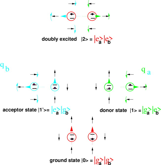
Figure 1: The reasons to use two modes; coupled chromophores (circles) can be both in ground (lower plot) state, or in a one-exciton state when either one of the chromophores is excited (left and right plots), or doubly excited state (upper plot); The monomer’s static dipoles $\vec{D}_{a}$, $\vec{D}_{b}$ (thick arrows) change for excited states; The equilibrium orientation of inter- and intra- molecular nuclear configuration (e.g. solvent librations - small arrows) reorganizes in order to compensate for the change of $\vec{D}_{a}$, $\vec{D}_{b}$.

Since the donor and acceptor chromophores are coupled to the intramolecular vibrations and collective nuclear modes of the environment, the equilibrium configuration of aforementioned modes depend on the electronic state of the dimer as illustrated in Fig. 1. Only two modes are taken due to following reason: According to Forster foer65 , for a dimer, the configuration of the nuclear subsystem is characterized by two Franck-Condon active modes $q_{a}$ and $q_{b}$ with frequencies of the order of benzene stretch mode. Note that in multidimensional configuration space representing orientations, vibrational and other degrees of freedom we choose just the elongations (and stretches) that accompany the change of equilibrium; and refer to them as to two reaction coordinates.

The difference in the equilibrium elongations of nuclear coordinates, corresponding to the ground $\left|0\right\rangle=\left|g_{a}\right\rangle\left|g_{b}\right\rangle$ and excited $\left|1\right\rangle=\left|q_{a}\right\rangle\left|e_{a}\right\rangle$ (donor), $\left|1^{\prime}\right\rangle=\left|g_{a}\right\rangle\left|e_{b}\right\rangle$ (acceptor) states of the dimer characterize the strength of the electron-phonon coupling kili04 . For doubly excited state $\left|2\right\rangle=\left|e_{a}\right\rangle\left|e_{b}\right\rangle$ bath modes are elongated equally. A symbol $d$ stands for the value of this elongation. The Hamiltonian of this dimer complex reads

$$H=\left|0\right\rangle H_{0}\left\langle 0\right|+\left|1\right\rangle H_{1}\left\langle 1\right|+\left|1^{\prime}\right\rangle H_{1^{\prime}}\left\langle 1^{\prime}\right|+\left|2\right\rangle H_{2}\left\langle 2\right|+D,$$ (1)

Here $D=J\{\left|1^{\prime}\right\rangle\left\langle 1\right|+\left|1\right\rangle\left\langle 1^{\prime}\right|\}$ stands for dipole-dipole coupling, $H_{j}$ for nuclear Hamiltonians:

$$H_{j}=\frac{p_{a}^{2}}{2m}+\frac{p_{b}^{2}}{2m}+v_{j}(q_{a},q_{b}).$$ (2)

Here we assume that potential energy surfaces $v_{j}(q_{a},q_{b})$ are harmonic and have the same frequency $\omega_{vib}$ and mass $m$ for each mode and each state cina05 .

$$v_{0} = \frac{m\omega^{2}}{2}\left(q_{a}^{2}+q_{b}^{2}\right),$$

$$v_{1} = \epsilon_{1}+\frac{m\omega^{2}}{2}\left([q_{a}-d]^{2}+q_{b}^{2}\right),$$

$$v_{1^{\prime}} = \epsilon_{1^{\prime}}+\frac{m\omega^{2}}{2}\left(q_{a}^{2}+[q_{b}-d]^{2}\right),$$

$$v_{2} = \epsilon_{2}+\frac{m\omega^{2}}{2}\left([q_{a}-d]^{2}+[q_{b}-d]^{2}\right),$$ (3)

The expression for reorganization energy reads

$$\Lambda=\frac{m\omega^{2}}{2}d^{2},$$ (4)

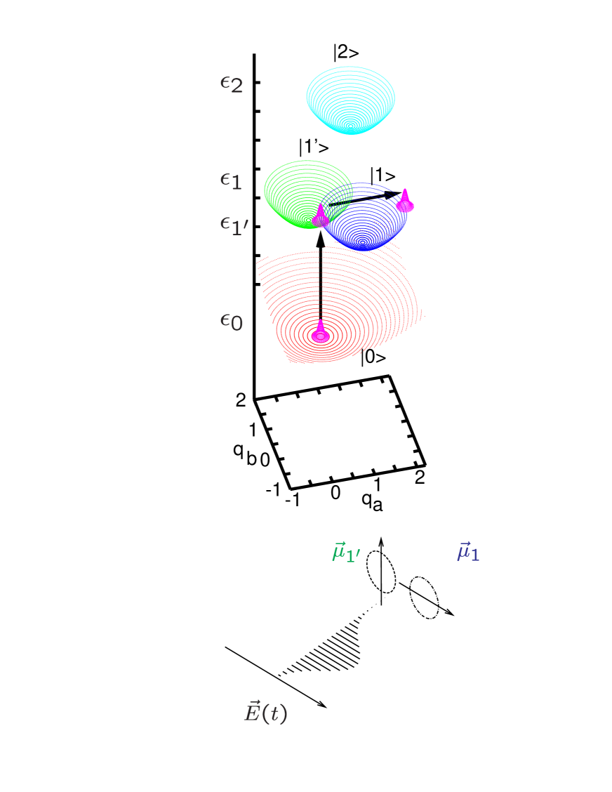
Figure 2: Potential surfaces of dimer illustrating equation 3 (upper plot); an example of mutual spatial orientation between laser pulse Eq. 5 and transition dipoles of dimer’s species Eq. 6 (lower plot)

and also referred to as ”Franck-Condon Energy” $E_{\rm FC}$. Figure 2 displays these potential surfaces $v_{j}(q_{a},q_{b})$ and ground state nuclear wavepacket promoted to the state $\left|1\right\rangle$ by one ultrashort pulse from the sequence

$$V_{I}(t) = -\hat{\mu}\vec{E}_{I}(t),$$

$$\vec{E}_{I}(t) = \vec{e}_{I}A_{I}(t-t_{I})\cos[\Omega_{I}(t-t_{I})+\Phi_{I}],$$ (5)

where $\vec{e}_{I}$, $A_{I}$, $t_{I}$, $\Omega_{I}$, and $\Phi_{I}$ stand for pulse polarization, envelope function, arrival time, frequency, and phase, respectively. $V_{I}$ and $\vec{E}_{I}$ symbolize interaction energy and laser field strength. The dimer electronic dipole moment

$$\hat{\mu}=\vec{\mu}_{a}\left(\left|1\right\rangle\left\langle 0\right|+\left|2\right\rangle\left\langle 1^{\prime}\right|\right)+\vec{\mu}_{b}\left(\left|1^{\prime}\right\rangle\left\langle 0\right|+\left|2\right\rangle\left\langle 1\right|\right)+H.c.$$ (6)

allow transitions in which the exciton number changes by one. Here it is assumed that there is no orientational disorder and the molecular dipoles $\vec{\mu}_{a}$ and $\vec{\mu}_{b}$ are not parallel, so that pulses of different polarization can selectively address donor $\left|1\right\rangle$ or acceptor $\left|1^{\prime}\right\rangle$ state. Restricting ourselves by rotating wave approximation and narrow envelope limit $A_{I}\sim\delta(t-t_{I})$, one can account for the first order of the laser pulse – dimer interaction resulting in the pulse propagation operator

$$I=e^{-i\int(H+V_{I})dt} \simeq \hat{1}+\int\limits_{-\infty}^{\infty}e^{-iH(t_{I}-t)}V_{I}(t)e^{-iH(t-t_{I})}dt.$$ (7)

Here $I$ labels the pulse in the sequence and equals to $A$, $B$, … for first, second, … pulse in a sequence. Subscript ”x” or ”y” of pulse label denotes its linear polarization that match $\vec{\mu}_{a}$ and $\vec{\mu}_{b}$, respectivly. Note, that $\vec{\mu}_{a}$ and $\vec{\mu}_{b}$ also must not be perpendicular in order to allow for the dipole-dipole transition $J$.

II.2 Calculation of quantum dynamics

After the Gaussian nuclear state has been promoted to the donor surface it starts to evolve in time with possibility of the transfer to the acceptor. We calculate this dynaics on quantum level For the sake of convenience the dimer Hamiltonian (1) is rewritten in the basis of harmonic oscillators eigenstates.

$$H_{j} = \epsilon_{j}+\hbar\omega(1/2+N_{j}+1/2+M_{j}),$$

$$D = J\sum_{M_{1^{\prime}}}\sum_{N_{1^{\prime}}}\sum_{M_{1}}\sum_{N_{1}}F_{FC}(1^{\prime}M_{1^{\prime}}N_{1^{\prime}};1M_{1}N_{1})\left|1M_{1}N_{1})\right\rangle\left\langle 1^{\prime}M_{1}^{\prime}N_{1}^{\prime}\right|.$$ (8)

Here $M_{j}$, $N_{j}$ stand for vibrational quantum numbers, $\left|jM_{j}N_{j}\right\rangle$ for nonadiabadic eigenstates of the dimer refered to as ”diabatic”, $F_{FC}(1^{\prime}M_{1^{\prime}}N_{1^{\prime}};1M_{1}N_{1})$ for Franck-Condon factors, describing overlaps of the wavefunctions that belong to different potential surfaces.

The diagonalization of the Hamiltonian (8) gives the set of $k=1..k_{\max}$ eigenenergies $\{\lambda_{k}\}$ and the set of $k_{\rm max}$ relevant eigenvectors $\vec{v}^{\tilde{l}}$ combined in a form of the transfer matrix $T_{k}^{l}$. The selected column $\tilde{l}$ of this matrix gives the elements of the $\tilde{l}$-th eigenvector $T_{k}^{\tilde{l}}=(\vec{v}^{\tilde{l}})_{k}$ in the diabatic basis. So that the solution of Schrödinger equation in diabatic state reads:

$$\psi^{\rm dia}_{k}=\sum_{l}\psi_{l}^{\rm eig}(0)T^{l}_{k}\exp\{-i\lambda_{l}t\}.$$ (9)

Here $\psi^{\rm eig}_{l}(0)$ stands for the wavefunction at the initial moment of time expressed in the eigenstate basis:

$$\psi^{\rm eig}(0)=T^{-1}\psi^{\rm dia}(0).$$ (10)

Here the wavefunction is represented through a diabatic state expansion

$$\left|\psi\right\rangle=\sum_{jM_{j}N_{j}}\psi^{\rm dia}_{jM_{j}N_{j}}\left|jM_{j}N_{j}\right\rangle,$$ (11)

where three indices can be combined into one ”superindex” $k$.

$$k=jN_{\rm max}^{2}+N_{j}N_{\rm max}+M_{j},$$ (12)

here only $j=0$ for state $\left|1\right\rangle$, $j=1$ for state $\left|1^{\prime}\right\rangle$, $N_{j}$ counts for number of vibrational quanta in a-mode, $M_{j}$ counts for the number of vibrational excitations in b-mode. The maximal number of vibrational excitations $N_{\rm max}$ varied between 17 and 20. To achieve the highest numerical precision at shorter computational time we have applied so called cut-off ansatz to the vibrational basis set. Namely $M+N\leq\tilde{N}$, $\tilde{N}$ -cutoff limit, $M$, $N$ stand for the number of quanta in $q_{a}$, $q_{b}$ modes, respectively.

Unless otherwise stated the diabatic initial wavefunction is taken to be coherent state in the donor potential well:

$$\psi^{\rm dia}_{jMN}=\delta_{j,1}e^{-\alpha^{*}\alpha/2}\sum_{M}\frac{\alpha^{M}}{\sqrt{M!}}e^{-\beta^{*}\beta/2}\sum_{M}\frac{\beta^{N}}{\sqrt{N!}}\left|jMN\right\rangle$$ (13)

Where $\alpha$, $\beta$ stand for amplitudes of coherent states in a-mode and b-mode, whose initial values are characterized by amplitudes $|\alpha|$, $|\beta|$ and phases $\phi_{a}$, $\phi_{b}$. In most cases tha amplitudes are expressed as integer multiples of $\delta=\sqrt{\frac{m\omega}{2}}d$. Since there are four potentials, where one can define a coherent state, it is important to have a unified description: The amplitudes $\alpha$,$\beta$ are defined so that $\alpha=0$, $\beta=0$ corresponds to ground vibrational state in this potential.

The definition of $\alpha$,$\beta$ depends on potential surface. The mean coordinate of the wavepacket does not depend on potential (on electronic state). The amplitude of coherent state $\alpha_{0}$, $\beta_{0}$ in ground potential has one-meaning correspondence with the mean coordinate $q_{a}$,$q_{b}$. In order to get a unified description one may represent the coherent state of any potential in the basis of the ground potential; by adding the displacement between relevant potentials in amplitude space $\delta=\sqrt{\frac{m\omega}{2}}d$.

The transfer matrix in Eq. 9 requirres some comments: The upper index $l$ enumerates the eigenstates, while the lower index comprises for diabatic one-exciton states and combines three quantum numbers as defined in Eq. 12:

II.3 Output variables

The transfer of the electronic population to acceptor is

$$P_{1^{\prime}}(t)=\sum_{MN}\psi^{*}_{1^{\prime}MN}\psi_{1^{\prime}MN}.$$ (14)

In order to study the wavepacket interferometry signal, we have convoluted the wavefunctions $\tilde{\psi}$, $\psi$, prepared by different pulses:

$$C_{DA}=\sum_{MN}\tilde{\psi}_{1^{\prime}MN}\psi_{1^{\prime}MN}.$$ (15)

The donor-, acceptor-, or the whole one-exciton wavefunction are

$$\psi_{j}(q_{a},q_{b}) = \left\langle j\right|\left\langle q_{a},q_{b}\right|$$ (16)

$$= \sum_{M_{j}}\sum_{N_{j}}\psi_{jM_{j}N_{j}}H^{a,j}_{M_{j}}(q_{a})H^{b,j}_{N_{j}}(q_{b}),$$

$$\psi^{\rm 1-exciton}(q_{a},q_{b}) = \psi_{1}+\psi_{1^{\prime}}.$$ (17)

Here 1-D harmonic oscillator eigenfunctions in coordinate representation for $j$-th potential surface are denoted $H^{a,j}_{M_{j}}(q_{a})$ and $H^{b,j}_{N_{j}}(q_{b})$ for a-mode and b-mode, respectively.

III Dynamics

III.1 Elementary act of transfer

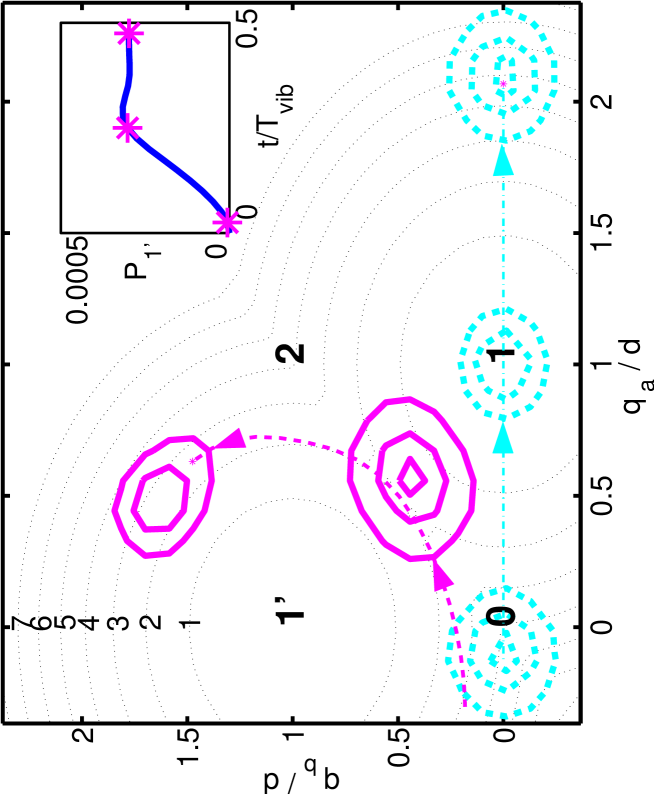
Figure 3: Elementary act of the electronic energy transfer; Contour lines of probability density wavepackets: $|\psi_{1}|^{2}$ - in donor potential (thick dashes), and $|\psi|^{2}$ - in acceptor potential (thick solid lines) are displayed at different time slices $t=0$, $t=\tau_{\rm vib}/4$, and $t=\\ tau_{\rm vib}/2$; inset shows the correspondent population kinetics, stars correspond to the time slices; ridge line $q_{a}=q_{b}$ connects ”0” and ”2”; $\epsilon_{1}-\epsilon_{1^{\prime}}=0$, $J=\omega/100$

The simplest scenario of the electron energy transfer dynamics takes place after the dimer gets excited by the short pulse with narrow envelope function $A(t)$, so that $\left|0\right\rangle$-surface ground vibrational state is safely translated up to one-exciton surface. The pulse polarization $\vec{e}$ is specifically matched $\vec{e}\perp\vec{\mu}_{b}$ to the dimer transition dipoles so that only donor surface gets excited into the Franck-Condon region, as shown in Fig. 3.

Since donor surface minimum is shifted just along $q_{a}$ though the donor wavepacket $|\psi_{1}(q_{a},q_{b})|^{2}$ starts oscillations along this coordinate. At the time ${\cal A}\tau$ wavepacket center comes closer to the ”ridge” region, defined by

$$q_{b} = q_{a}-\frac{\epsilon_{1}^{\prime}-\epsilon_{1}}{m\omega^{2}d},$$ (18)

$$\nu_{1}(q_{a},q_{b}) = \nu_{1^{\prime}}(q_{a},q_{b}).$$

The correspondent Franck-Condon window provides that part of the donor wavepacket amplitude is transferred to the acceptor surface. The wavefunction amplitude in the acceptor state grows by small increment, linearly proportional to the intensity of the dipole-dipole coupling $J$. The transferred portion of the wavepacket, $\psi_{1}^{\prime}(q_{a},q_{b})$ maintains the mean coordinate and momentum at the time of the elementary act, but, afterwards the motion of this portion of the amplitude is governed by the nuclear Hamiltonian $H_{1^{\prime}}$.

For this specific Franck-Condon-excitation of $a$-mode the transfer takes time at

$${\cal A}\tau=\frac{1}{\pi}\arccos\left(1-\frac{\epsilon_{1}-\epsilon_{1^{\prime}}}{m\omega d^{2}}\right).$$ (19)

The mean position of the acceptor wavepacket

$$\bar{q}_{l}(t)=\frac{\int\int dq_{a}dq_{b}\psi_{1}^{\prime*}(q_{a},q_{b},t)q_{l}\psi_{1}^{\prime}(q_{a},q_{b},t)}{\int\int dq_{a}dq_{b}\psi_{1}^{\prime*}(q_{a},q_{b},t)\psi_{1}^{\prime}(q_{a},q_{b},t)},$$ (20)

performs elliptical motion about the acceptor potential surface minimum. During the time period that donor wavepacket stays apart from the ridge region there is no essential transfer of the amplitude, so the acceptor population kinetics remains flad, parallel to the time axis. It can be also calculated as follows:

$$\bar{q}_{a}(t) = \sqrt{\frac{\hbar}{2m\omega}}(\alpha+\alpha^{*}),$$

$$\alpha = \left\langle 1^{\prime},M_{1^{\prime}},N_{1^{\prime}}\right|\hat{a}\left|1^{\prime},M,N\right\rangle,$$

$$\hat{a} = \sum_{N}\sqrt{N}\left|N\right\rangle\left\langle N+1\right|.$$ (21)

III.2 Stepwise population dynamics

Since nuclear potentials are harmonic, the donor wavepacket performs cyclic motion with period $\tau_{\rm vib}=\frac{2\pi}{\omega_{\rm vib}}$ and comes to the ridge region regularly, once per vibrational period. Therefore, the elementary act of electronic energy transfer takes place repeatedly, once per vibrational period, as shown in Fig. 3. It is generally expected that quantum evolution of the coupled electronic states whose mutual detuning or coupling are modulated displays the stepwise character of population dynamics garr97 . For the short time or small coupling limit the almost equal portions of the wavefunction amplitude are transferred per vibrational period, therefore the acceptor wavefunction amplitude growth linear in time, but overall population growth of acceptor has a quadratic character

$$P_{1^{\prime}}(t)\sim 1/2(\exp[-\frac{1}{4}\frac{\Lambda}{\omega}])^{2}J^{2}t^{2}$$ (22)

for the short time limit $t\ll\frac{1}{2J}$.

III.3 Detunings

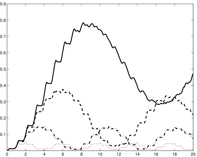
Figure 5: Population kinetics for different off-resonance detuning: $\epsilon_{1}-\epsilon_{1^{\prime}}=0$ (solid) $\epsilon_{1}-\epsilon_{1^{\prime}}=\omega/16$ (dashed) $\epsilon_{1}-\epsilon_{1^{\prime}}=\omega/8$ (dot-dashed) $\epsilon_{1}-\epsilon_{1^{\prime}}=\omega/4$ (dots)

Fig. 5 represents the acceptor state population kinetics $P_{1^{\prime}}(t)$ for slightly different site energies $\epsilon_{1}\sim\epsilon_{1^{\prime}}$. During first vibrational period the kinetics are indistinguishable. At longer times the off-resonant energy configurations provide higher frequency of electronic nutations (population oscillations) and diminishes their amplitude so that acceptor population never gets fully populated.

This result is in qualitative agreement with two coupled levels behavior $P_{DA}=A\sin^{2}\Omega_{\rm R}t$, where Rabi frequency $\Omega_{\rm R}=\sqrt{(\epsilon_{1}-\epsilon_{1^{\prime}})^{2}+4J^{2}}$ growth with detuning, and amplitude $A=\frac{J^{2}}{\Omega_{\rm R}^{2}}$ decreases with detuning.

III.4 Population dynamics at long time limit. Revivals

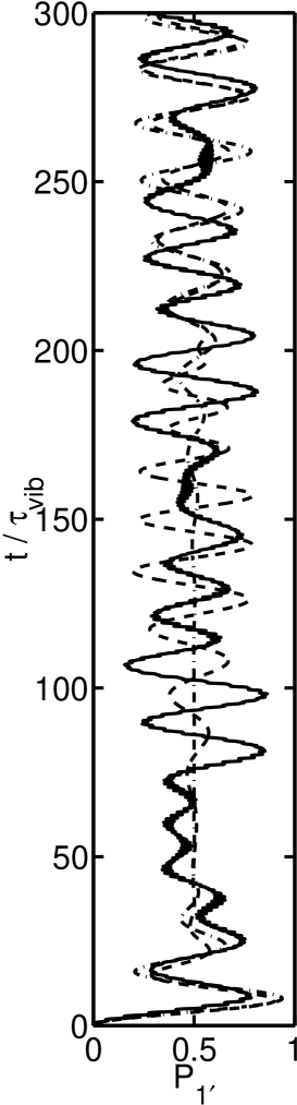
Figure 6: long-time population dynamics for $\epsilon_{1}-\epsilon_{1^{\prime}}=0$, $J=\omega_{\rm vib/10}$: collapses and revivals, simulation (solid) and equation 25 with two sets of parameters: $g=JE_{\rm FC}\sqrt{1/\omega}$, $\alpha=\sqrt{m\omega/2}d$ (dashed) and $g=JE_{\rm FC}\sqrt{2/\omega}$, $\alpha=\sqrt{m\omega}d$ (dot-dashed),

For the long time limit one expects clear and simple behavior of the population dynamics based on the extrapolation of the result for two coupled electronic states model rabi37 ; bloc46 ; alen73 ; muka95 , i.e. coherent oscillations of the population from donor to acceptor and back with Rabi frequency $\Omega_{\rm R}=\sqrt{(\epsilon_{1}-\epsilon_{1^{\prime}})^{2}+4J^{2}}$. However, we show in Fig. 6 that these oscillations dephase quickly to the state where donor and acceptor are equally populated $P_{1}=P_{1^{\prime}}=1/2$. This quasi-damping originates from the destructive interference: More specifically, each single level of donor potential (labelled by superindex $k\leq N_{\rm max}^{2}$) is coupled to different level of acceptor potential ($l>N_{\rm max}^{2}$).

The coupling strength $J\times{\rm FC}(l,k)$ differs for each pair. As long as many donor diabatic states are initially populated, (see Eq. 13), so that the total population of acceptor $P_{1^{\prime}}=\sum_{l>N_{\rm max}^{2}}|\psi_{l}|^{2}$ is constructed from the sum of many contributing terms (acceptor levels populations),

$$|\psi_{l}(t)| = \sum_{k\leq N_{\rm max}^{2}}\left[\frac{2J{\rm FC}(l,k)}{\Omega_{lk}}\right]^{2}\sin^{2}\left(\Omega_{lk}t\right)|\psi_{k}(0)|^{2},$$ (23)

oscillating with different frequencies

$$\Omega_{lk} = \sqrt{\left(H_{kk}-H_{ll}\right)^{2}+4J^{2}{\rm FC^{2}(l,k)}}.$$ (24)

This type of dynamics was originally revealed for a two-level atom resonantly coupled to one-mode electromagnetic field jayn63 . Inspite of different physical nature and different coupling operator the electronic population dynamics that has been calculated in this work can be fitted to the Jaynes-Cummings analytical formula

$$P_{1^{\prime}}=e^{-|\alpha|^{2}}\sum\limits_{N}\frac{|\alpha|^{2N}}{N!}\cos^{2}\left(g\sqrt{N+1}t\right).$$ (25)

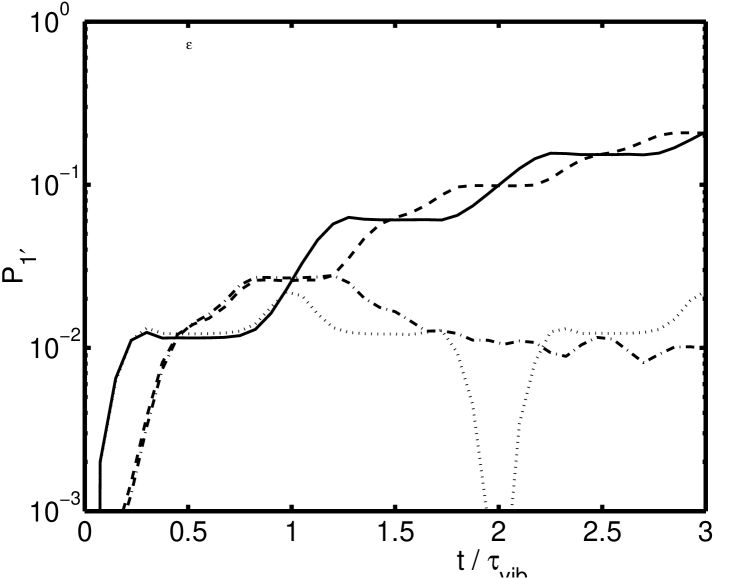
Figure 4: Short-time population dynamics for coupling strength $J=\omega/10$ and various energy configurations: $\epsilon_{1}-\epsilon_{1^{\prime}}=0$ (solid), $\epsilon_{1}-\epsilon_{1^{\prime}}=\omega/2$ (dashed), $\epsilon_{1}-\epsilon_{1^{\prime}}=7\omega$ (dotted), $\epsilon_{1}-\epsilon_{1^{\prime}}=7.39\omega=2E_{\rm FC}$ (dot-dashed); solid and dashed displays one step per vibrational period, dotted and dot-dashed dispaly two steps per vibrational period; since short time-population is small log-scale is used for $P_{1^{\prime}}$.

Here $g=\sqrt{J^{2}\Lambda^{2}/\omega_{\rm vib}}$ stands for analog of Jaynes-Cummings coupling strength. The calculated and empirical curves do coincide within collapse time interval. However, the revival of population difference occurs at different times for energy transfer system kili04 . Another difference is that energy transfer population changes by periodic steps, as shown before, in Fig. 4. These studies have close association with the numerical simulation on two-mode-field JCM model naka02 and with the Jahn-Teller effect cinaRaman00 .

For finite system, the behavior has well defined features, so there is reason to look for an analytical solution of exciton transfer dynamics in form

$$\left|\psi(t)\right\rangle = e^{-i(\hat{H}_{1}+\hat{H}_{1^{\prime}}+\hat{D})t}\left|\psi(0)\right\rangle,$$ (26)

by taking in to account commutation relations between $H_{1}$, $H_{1^{\prime}}$, and $D$.

III.5 Shrinking of mean trajectory

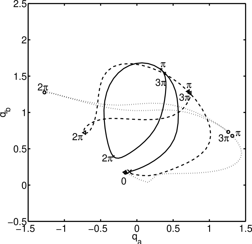
Figure 7: Trajectory of mean position of the target wavepacket for $\epsilon_{1}-\epsilon_{1^{\prime}}=0$ (solid), $\epsilon_{1}-\epsilon_{1^{\prime}}=E_{\rm FC}$ (dashed), $\epsilon_{1}-\epsilon_{1^{\prime}}=2E_{\rm FC}$ (dotted); during the time interval $0<\omega t<3\pi$

As shown in Fig. 7 the mal transfer region Eq. 18 determines the shape of the mean position trajectory of the target wavepacket. Starting close to the position $q_{a}=0$,$q_{b}=0$ the trajectories oscillate in both $q_{a}$ and $q_{b}$, thought the amplitude of these oscillations in the ”direction of transfer” growth with energy difference $\epsilon_{1}-\epsilon_{1^{\prime}}$. At the time $\omega t=\pi$ and $\omega t=3\pi$ each trajectory comes throught the same point.

Each time donor comes to the ridge region the wavefunction portion peeled to the acceptor potential is not exactly the same. Each cycle acceptor wavepacket spreads wider and wider. This spreading makes an imprint on the acceptor wavepacket mean position trajectory, as shown in Fig. 7. For equal site $\epsilon_{1}-\epsilon 1^{\prime}=0$ configuration this trajectory repeats without any changes in the direction

$$q_{||}=\frac{1}{\sqrt{2}}(q_{a}+q_{b})$$ (27)

and shrinks the amplitude of the oscillations along the line

$$q_{\perp}=\frac{1}{\sqrt{2}}(q_{a}-q_{b})$$ (28)

that connects the minimas of the potential surfaces.

The direction of trajectory shrinking depends on energy configuration, therefore it is an open question, whether the complete problem can be reformulated with just one vibrational mode, namley $q_{\perp}$.

To conclude this section we have three main findings related to the dynamical behavior of the system: Population transfer displays stepwise character in the short time limit and coolapse-revival character on the long-time scale. The mean acceptor trajectory shrinks in amplitude along the direction depending on site energy configuration (”line of the transfer”).

IV Static features

IV.1 The dependence of the population transfer on the vibrational trajectory

In our model dimer, either one or series of ultrashort polarized pulses is able to excite the donor potential surface into some two-dimensional coherent state Eq. 13. For example: As shown before, a single $x$-polarized pulse creates the coherent excitation in the $q_{a}$ mode having Franck-Condon amount of vibrational energy, placed initially at $(q_{a}=0,q_{b}=0)$ with initial phase $\phi_{a}=0$. However, the specific sequences of pulses can create vibrational excitations in donor surface, starting at different points of phase space. One of these examples is illustated below: Let’s consider the excitation prepared by a $y$-polarized pulse. After a quarter of vibrational period $\tau_{\rm vib}/4$ we send an x-pulse and, another quarter period later, a y-pulse. . This pulse sequence creates a two-dimensional circular motion about center of donor surface, having $4E_{FC}$ energy in both modes moving $2d$ apart from the center of donor surface, starting at point $q_{a}=d,$ $q_{b}=2d$. When the last pulse is applied half a period ($\tau_{\rm vib}/2$) later then it produces again the $q_{a}$ coherent excitation in a donor surface having, however no initial elongation but nonzero momentum giving an initial phase $\phi_{a}=3\pi/2$. This section shows that specific pulse series does create specific coherent states in a donor surface.

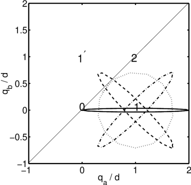
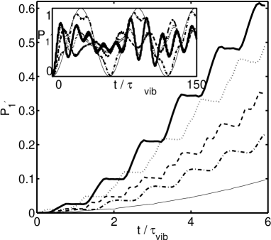
Figure 8: Dependence of transfer on the specifics of the vibrational excitation in donor surface: mean position trajectories of donor surface wavepacket (upper panel) and correspondent populations kinetics at short time (lower panel) and long time (inset of lower panel); $\epsilon_{1}-\epsilon_{1^{\prime}}=0$; $J=\omega/10$; for each trajectory the vibrational energy of $E_{\rm FC}$ is differently apportioned between nuclear modes: Franck-Condon excitation, $q_{\rm a}$-mode excited (solid line), $q_{\perp}$-mode excited (dashed line,) $q_{||}$-mode excited (dot-dashed line), circular excitation - both modes equally excited (dotted line); for the purpose of reference thin solid line on bottom panel correspond to ground nuclear state in donor potential; for better illustration $q_{\rm a}$, $q_{\perp}$, $q_{||}$ trajectories are prepared to have a small portion of vibrational energy in the adjacent coordinate.

The change of vibrational states in donor surface does affect the intensity of the electronic energy transfer to acceptor. To investigate this we have considered a set of coherent states having the same amount of vibrational energy ($E_{FC}$) differently apportioned between $q_{a}$ and $q_{b}$ modes, see Fig. 8. As shown before, the elementary act of transfer takes place when the wavepacket crosses the ridge region of potential energy landscape Eq. 18. The mean coordinate trajectories of different coherent states cross this line in a different manner. In accordance with Landau-Zener formula land32 ; zene32 , as longer the wavepacket stays on the ridge line as faster the population transfer goes.

The minimal intensity of the transfer is found for the intitial state of donor having no vibrational excitation at all (ground vibrational state). This initial state provides simple oscillations of electronic amplitude from donor $\left|1\right\rangle$ to acceptor $\left|1^{\prime}\right\rangle$ and back with frequency $J\times FC(1,0,0;1^{\prime},0,0)$ in leading order determined by Franck-Condon overlap of ground vibrational state of each potential. Vibrational trajectory in $q_{||}$ direction provides similar oscillatory behavior on the long time scale. Excitations of $q_{\rm a}$, $q_{\perp}$, and circular excitation lead to the quicker transfer on short time-scale and collapse-revivals behavior on the long time scale. It is clearly shown that presence of vibrational excitation enhances the transfer of electronic amplitude between one-exciton states.

IV.2 Origins of parallel, perpendicular and combined effect

The ridge region is intersecting the line connecting the minima of donor ($q_{a}=d$, $q_{b}=0$) and acceptor ($q_{a}=0$, $q_{b}=d$) surfaces. It is reasonable to measure the distance between wavepacket and the region of the optimal transfer along this line. Therefore we use the $45$ degrees rotated system of coordinates consisting of $q_{||}$ and $q_{\perp}$ coordinates, described by Eq. 27 and Eq. 28. The motion of a coherent wavepacket along $q_{\perp}$ is expected to determine the efficiency of the transfer. The dependence of population transfer on the motion in $q_{||}$ does remain to be an open question. Instead of taking an exhaustive collection of all possible two-dimensional states, in Eq. 13 we consider the set of vibrational states having different amount of excitation and phase along either $q_{\perp}$ or $q_{||}$, in order to exploit all available transfer regimes.

IV.3 Dependence on energy difference

As long as region of potentials’ intersection location Eq. 18 $q_{b}=q_{a}-\frac{\epsilon_{1}-\epsilon_{1^{\prime}}}{m\omega^{2}d}$ depends on site-energy difference between donor and acceptor moieties, the efficiency of the population transfer is expected to depend on the difference $\epsilon_{1}-\epsilon_{1^{\prime}}=E_{DA}$. The dependence on energy difference gives a sence how The energy Specific rolecules in specific solvents give various regimes of energy difference. By scanning all values of energy difference we get a sence of behavior of various real systems.

IV.3.1 The role of pendicular excitation.

It follows from Fig. 8 that the presence of vibrational energy in $q_{\perp}$ - mode gives rise to the population transfer. There is also no strong dependence on energy difference $E_{DA}=\epsilon_{1}-\epsilon_{1^{\prime}}$ because almost any position of the intersection line Eq. 18 $q_{b}=q_{a}-(\epsilon_{1}-\epsilon_{1^{\prime}})/m\omega^{2}d$ is reachable by $q_{\perp}$-coherent wavepacket. The intersting dependence of population transfer on the phase of $q_{\perp}$ coherent motion is left to consider later.

IV.4 Dependence on parallel excitation

IV.4.1 Introduction of Fock states

The dependence of population transfer on the excitation of the $q_{||}$ mode is rather small. Therefore,we do not consider the initial phase of of the $q_{||}$ excitation but only the amount of vibrational energy in this mode. The relevant state with the definite number of vibrational quanta is so-called Fock-state with $P$ vibrational quanta in $q_{||}$ mode. In the basis of the natural vibrational quantum numbers $M,N$ for the modes $q_{a}$, $q_{b}$ this state reads:

$$\psi^{Fock}(1,M,N)=\frac{\partial^{M}}{\partial q_{||}^{M}}\frac{\partial^{N}}{\partial q_{\perp}^{N}}\left\langle q_{a}\right|\left|0\right\rangle\left\langle q_{b}\right|\left|0\right\rangle.$$ (29)

Here $\left\langle q_{a}\right|\left|0\right\rangle=\psi_{0}(q_{a})$ $\left\langle q_{b}\right|\left|0\right\rangle=\psi_{0}(q_{b})$ stand for ground states in each vibrational modes. Since the common ground state is factor of those two, one gets two dimensional $M,N$-Fock states in $q_{||}$, $q_{\perp}$ by applying the derivatives along these coordinates M and N times, respectively.

$$\frac{\partial^{M}}{\partial q_{||}^{M}} = \left\{\frac{1}{\sqrt{2}}\frac{\partial}{\partial q_{a}}+\frac{1}{\sqrt{2}}\frac{\partial}{\partial q_{b}}\right\}\left\langle q_{a},q_{b}\right|\left|0\right\rangle,$$ (30)

$$\frac{\partial^{M}}{\partial Q_{\perp}^{M}} = \left\{-\frac{1}{\sqrt{2}}\frac{\partial}{\partial Q_{a}}+\frac{1}{\sqrt{2}}\frac{\partial}{\partial Q_{b}}\right\}\left\langle q_{a},q_{b}\right|\left|0\right\rangle.$$

IV.5 Overall Markus’ hump analysis

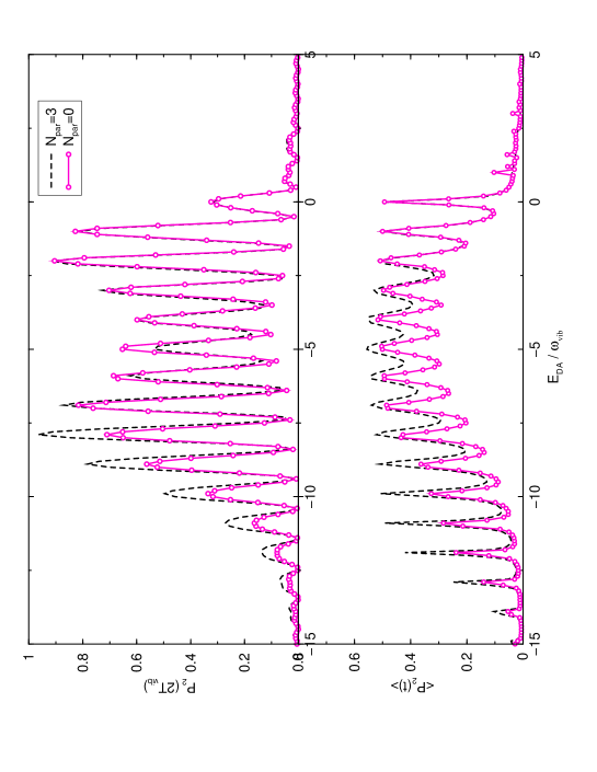
Figure 9: Electronic energy transfer to acceptor state for various site energy differences for $J=\omega/2$; solid line with circles stands for zero-point vibrations in donor surface (no vibrations), dashed line - Fock state excitation in donor surface, upper panel shows population of $\left|1^{\prime}\right\rangle$ at $t=2\tau_{\rm vib}$, lower panel shows acceptor population averaged over $T=100\tau_{\rm vib}$: $\bar{P}_{1^{\prime}}=\frac{1}{T}\int\limits_{0}^{\infty}P_{1^{\prime}}(t)dt$

The simplest vibrational state is the ground state, having no vibrational quanta at all. For this state the dependence of acceptor population on energy difference $E_{DA}=\epsilon_{1}-\epsilon_{1^{\prime}}$ has no admixture of vibrational influence, as shown in Fig. 9. This dependence has a form of overall hump, modulated by fringe-like srtucture. The overall hump has maximum at $E_{DA}=\epsilon_{1}-\epsilon_{1^{\prime}}=-2E_{FC}$, where the acceptor diabatic potential surface crosses the minimum of the donor potential surface. This corresponds to the activationless regime of the electron transfer with one reaction coordinate in the Marcus theory, which has an enormous range of applications to exciton, electron, proton transfer and many other chemical reactions mark86 ; kili99 ; foer65 ; kuhn_may ; schatz-ratner-book . The fringes originate from the individual resonances between vibrational levels, belonging to donor and acceptor moieties. The presence of theese individual resonances support the discussion in section III.3 and Eq. 23. Up to our knowlege such fringes were at first noted for one-mode system fuchs96 .

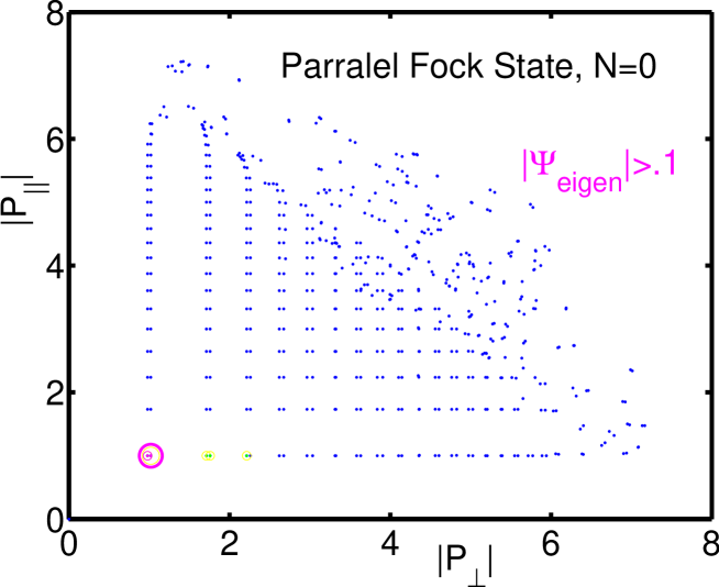
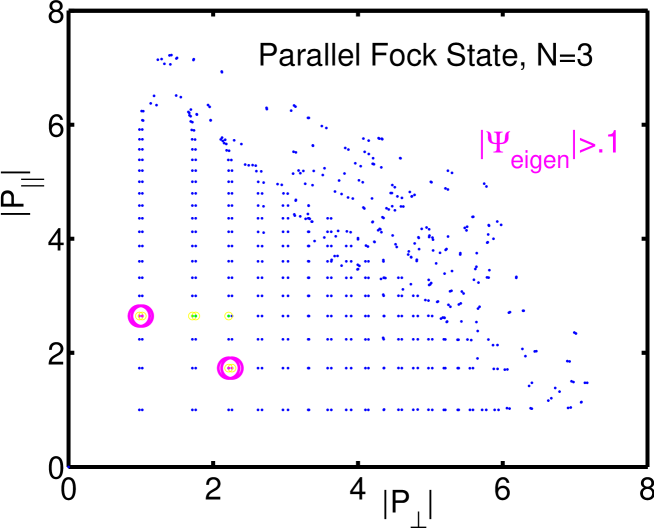
Figure 10: Mean values of momenta for 1-exciton eigenstates $\left|l\right\rangle$; each dot correspond to one eigenstate; horizontal position corresponds to the value of $\left\langle l\right|p_{\perp}|\left|l\right\rangle$; vertical position corresponds to the value of $\left\langle l\right|p_{||}|\left|l\right\rangle$ here $\epsilon_{1}-\epsilon_{1^{\prime}}=0$, $J=\omega/10$; The $J$-coupling strength induces splitting in the direction of transfer.

For large value of energy difference, vibrational Fock-state in the $q_{||}$-mode provides faster population transfer than the ground vibrational state of the donor potential. In order to understand this effect an eigenstate analysis has been performed. As far as one knows the vibronic eigenstates of the dimer, it is possible to find the mean values of some relevant variables, (like e.g. mean coordinate in Eq. 21). For example, the mean values of momentum $p_{||}=m\dot{q}_{||}$ and $q_{\perp}=m\dot{q}_{\perp}$ are calculated systematically for all eigenstates and develop a regular structure displayed in Fig. 10.

The diabatic ground state and a Fock-state in donor surface were expanded over eigenstates basis set

$$|\psi_{ground}>=\sum_{\nu}P^{ground}_{\nu}|\nu>,$$ (31)

$$|\psi_{Fock}>=\sum_{\nu}P^{Fock}_{\nu}|\nu>.$$ (32)

and displayed in Fig. 10. Here $\left|\nu\right\rangle$ stands for $\nu$-th eigenstate. The set of mean momenta enumerates eigenstates. The ground diabatic state involves the eigenstate that has minimal mean momenta. The ”parallel Fock state” does not have any vibrational excitations in $q_{\perp}$ direction. That is why it is expected to employ just those eigenstates with larger mean values of $p_{||}$. In contrast, the numerical simulation shows, that this state employ some eigenstates with large momentum $p_{\perp}$ in ”perpendicular” direction. The presence of such states in the eigenstate expansion of the Fock-state is, probably, responsible for the difference in population transfer rates, provided by these two diabatic vibrational states.

IV.6 The role of perpendicular phase

IV.6.1 Specific values of phase

We return back to the dependence on excitation of $q_{\perp}$ mode. The challenging question is whether the transfer rate depends on the amount of vibrational energy in this mode only or not. Alternativly, it can depend on the initial phase of the $q_{\perp}$ -coherent excitation in donor manifold. We demonstrate the results for two most distinctive cases: Wavepacket is far apart from the intersection ridge ($\phi_{\perp}=0$) and the opposite position ($\phi_{\perp}=\pi$) that stays at closest to the acceptor surface minimum. $\alpha=\delta e^{i\frac{\pi}{2}}$, $\beta=\delta e^{-i\frac{\pi}{2}}$ and …

IV.6.2 Evident results

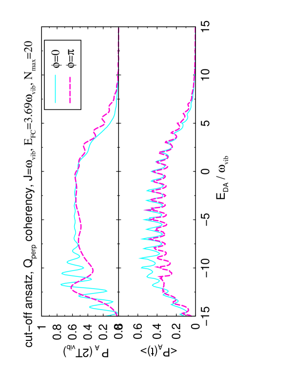
Figure 11: Electronic energy transfer to acceptor state $\left|1^{\prime}\right\rangle$ as function of energy configuration calculated for initial vibrational excitation of $q_{\perp}$-mode having $E_{\rm FC}$ of vibrational energy in donor potential; initially posiitoned apart from acceptor ($\phi=0$, solid), or close to acceptor ($\phi=\pi$, dashes); for $\epsilon_{1}-\epsilon_{1^{\prime}}<0$ $\phi=0$ provides faster transfer than $\phi=\pi$ for $\epsilon_{1}-\epsilon_{1^{\prime}}<0$ $\phi=0$ provides slower transfer than $\phi=\pi$.

Figure 11 shows that there is small but evident distinction in population transfer, corresponding to this two cases. For positive site-energy difference $E_{DA}=\epsilon_{1}-\epsilon_{1^{\prime}}>0$ referred to as ”uphill transfer” the coherent state initially positioned in the acceptor region provides quicker transport. For negative site energy difference difference $E_{DA}=\epsilon_{1}-\epsilon_{1^{\prime}}<0$, referred to as ”downhill transfer” manc04 , the quicker transfer occurs to be for the coherent state, initially placed in the region of donor surface minimum.

IV.7 Explanation to repositioning of adiabatic potential

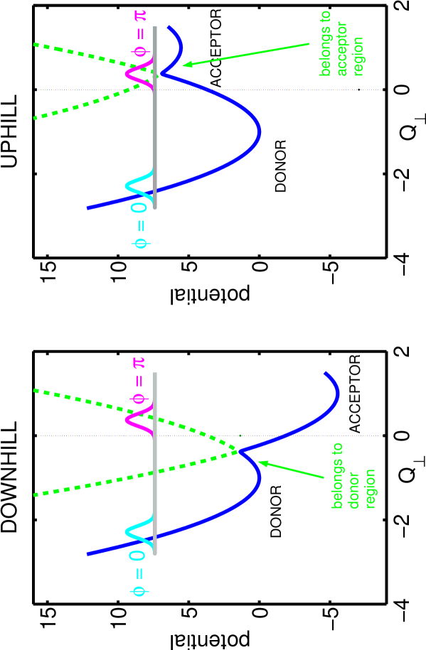
Figure 12: Schematic illustration of adiabatic potentialenergy surfaces Eq. 33 for $\epsilon_{1}-\epsilon_{1^{\prime}}<0$ (left panel) and for $\epsilon_{1}-\epsilon_{1^{\prime}}<0$ (right panel) solid line stands for lower potential $\nu_{-}$, dashed line stands for upper panel $\nu_{+}$; gaussian profile symbolizes the initial vibrational state in donor potential surface: having zero phase of $q_{\perp}$ excitation (left), or having $\pi$ phase of $q_{\perp}$ excitation (right).

The difference in the transfer rate becomes transparent while analyzing wavepackets’ motion in the adiabatic potentials, as shown in Fig. 12. The analysis is based on the fact that the actual wavepacket motion takes place in the upper and lower adiabatic surfaces

$$\nu_{\pm}(q_{a},q_{b}) = \frac{\nu_{1}+\nu_{1^{\prime}}}{2}\pm\sqrt{\left(\frac{\nu_{1}-\nu_{1^{\prime}}}{2}\right)^{2}+4J^{2}}.$$ (33)

Therefore, the time evolution of this system depends on how the initial wavepacket is repartitioned between upper $\nu_{+}$ and lower $\nu_{-}$ adiabatic potentials. For given mean position and mean energy of wavepacket the largest part belong to the surface that have the closer energy value at this position. For any energy difference the wavepacket $\phi_{\perp}=0$ belongs to the lower potential, while the wavepacket with shifted phase $\phi_{\perp}=\pi$ belongs to the upper potential and is confined there.

The only difference between ”uphill” and ”downhill” transfer is the position of the minimum of the upper adiabatic potential. As shown in Fig. 12 this minimum is shifted aside of donor or acceptor, for downhill and uphill cases, respectively.

For downhill transfer the $\phi_{\perp}=\pi$ wavepacket stays longer in donor region, therefore the transfer to acceptor is diminished. For uphill transfer the $\phi_{\perp}=\pi$ wavepacket stays longer in acceptor region and so provides the faster transfer with respect to the transfer corresponding to the $\phi_{\perp}=0$ coherent vibration.

In this section has been revealed that energy transfer depends on regime of launched wavepacket passing through the cotential-crossing region of energy landscape mostly associated with amplitude of motion along the line connecting the potential minima.

V Detection

V.1 General principles

There has been discussed nontrivial features of energy transfer channel of photoexcitation (evolution / decay) in dimers that would be interesting and relevant to reflect by means ultrafast spectroscopical measurements.

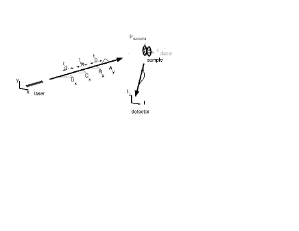
Figure 13: Schematic representation of interferometry experiment; ensamble of dimers with specific spatial orientation (of transition dipoles $\mu_{\rm donor}$ and $\mu_{\rm acceptor}$) is labelled as ”sample”; ”laser setup” generates four short pulses, resonant to dimer excitation frequency, pulses are labelled with capital letters, subscript ”x” or ”y” indicates pulse polarization; time delays between pulses are labelled as $t_{\rm p}$, $t_{\rm w}$, $t_{\rm d}$, where subscripts p, w, d abbreviate for ”preparation”, ”waiting”, and ”delay”, respectivly; excited sample’s polarized fluorescence is measured with ”detector”; only the fluorescence part with polarization attributed to ”acceptor” chromofore is analyzed in the text.

In this section, we discuss the novel measurement scenario, allowing to get wavefunction-amplitude-level information about exciton transfer and nuclear dynamics in molecular dimers. This scenarion requires four polarized-pulse excitations. In order to be concrete we choose the specific number of pulses and polarization arrangements: four pulses $A_{y}B_{x}C_{x}D_{x}$ separated by preparation $t_{\rm p}=t_{B}-t_{A}$, waiting $t_{\rm w}=t_{C}-t_{B}$, and delay $t_{\rm d}=t_{D}-t_{C}$ times, respectivly cina2002 ; jona03 . As displayed in Figure 13, our ”observable” is the $I_{||}$ component of the fluorescence from the oriented sample that has been excited by aforeshown pulse sequence. The $I_{||}$ fluorescence intensity is proportional to the population of the acceptor state $\left|1^{\prime}\right\rangle$ of the dimer. There are few elementary laser-molecule interaction processes that give rise to the population of the state. All but nonlinear (depending on all four pulses) processes can be cutted off out by applying mechanical choppers sche91 ; sche92 .

Among the rest of the nonlinear processes we consider only those quadrrilinear in the intensities of each pulse because they are of larger value

$$P_{1^{\prime}}(A_{y}B_{x}C_{x}D_{x})=2\Re\left\{\right.\left\langle 1^{\prime}\right| \left\langle A_{y}\right|\left|JD_{x}C_{x}B_{x}\right\rangle e^{-i\phi_{p}-i\phi_{d}}$$ (34)

$$\left\langle A_{y}\right|\left|D_{x}C_{x}JB_{x}\right\rangle e^{-i\phi_{p}+i\phi_{d}}$$

$$\left\langle D_{x}C_{x}A_{y}\right|\left|JB_{x}\right\rangle e^{-i\phi_{p}-i\phi_{d}}$$

$$\left\langle D_{x}B_{x}A_{y}\right|\left|JC_{x}\right\rangle$$

$$\left\langle C_{x}B_{x}A_{y}\right|\left|JD_{x}\right\rangle\left|1^{\prime}\right\rangle\left.\right\}.$$

Note that in this polarisation scheme all contributions to $P_{1^{\prime}}=\left\langle\psi_{1^{\prime}}\right|\left|\psi_{1^{\prime}}\right\rangle$ depend on exciton transfer. Linearly combining some quadrilinear fluorescence signals taken with different relative phase-locking angles $\phi_{p}$, $\phi_{d}$ between $A_{y}B_{x}$ and $C_{x}D_{x}$ pulses as described in cina2002

$$\left<\left(A_{y}\right)_{1^{\prime}}\right.\left|\left(D_{x}C_{x}JB_{x}\right)_{1^{\prime}}\right>^{(0)} =$$

$$\frac{1}{4}\left\{P_{1^{\prime}}\left({0,0}\right)-P_{1^{\prime}}\left({\frac{\pi}{2},-\frac{\pi}{2}}\right)+iP_{1^{\prime}}\left({\frac{\pi}{2},0}\right)-iP_{1^{\prime}}\left({0,\frac{\pi}{2}}\right)\right\}$$

one gets the value that can be taken in to account by the double side Feynman diagram weis89 ; muka95 shown in Fig. 14. Here the left side describes so-called ”target” wavefunction, where the population amplitude in state $\left|1^{\prime}\right\rangle$ is promoted from the ground state by three pulses $B_{x}$, $C_{x}$, $D_{x}$ and one primariy electronic energy transfer act between $B_{x}$ and $C_{x}$ pulses. Here the vertices of the fiagram are given by linear terms of pulse propagators 7.

The actual population of state $\left|1^{\prime}\right\rangle$ (and fluorescence from it) is proportional to the coincidence between ”target’ and so-called ”reference” wavepacket, schematically presented by the right part of the Feynmann diagram and promoted from the ground state to the $\left|1^{\prime}\right\rangle$ by a single $A_{y}$ pulse.

As long as electronic transitions in this model dimer are coupled to the nuclear modes, the probability amplitude wavepackets change their positions and may not coincide for the left and right part of the diagram. This argument gives reason to expect essential interference population of $\left|1^{\prime}\right\rangle$ for some specific values of time delays only.

V.2 Equal site energies versus downhill

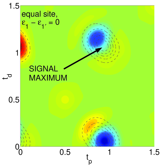
Figure 15: Real part of the interferometry signal provided by $\left\langle A_{y}D_{x}C_{x}\right|\left|JB_{x}\right\rangle$ - process for $\epsilon_{1}-\epsilon_{1^{\prime}}=0$ energy configuration as function of delay times $t_{p}$, $t_{d}$ between pulses; dark areas correspond to negative signal, bright areas correspond to positive signal, contour dashed lines display the absolute value of the signa; the signal has main maximum aleft far of the diagonal repeating periodically at integer multiples of $t_{p}$, $t_{d}$ with slow change of the sign yelding three fringes: oscillation frequency $-0.53\omega$ along $t_{p}$, $0.53\omega$ along $t_{d}$; there is also small satellite peak at $t_{p}=0.5\tau_{\rm vib}$, $t_{d}=0.5\tau_{\rm vib}$.

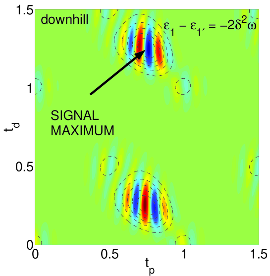
Figure 16: Real part ofthe interferometry signal provided by $\left\langle A_{y}D_{x}C_{x}\right|\left|JB_{x}\right\rangle$ - process for $\epsilon_{1}-\epsilon_{1^{\prime}}=2E_{\rm FC}$ enegry configuration as function of delay times $t_{p}$, $t_{d}$ between bulses A, B and C, D, respectivly; dark - negative signal, bright - positive signal, dashed contours - amplitude of signal; the signal maximum at $t_{p}=0.75\tau$, $t_{d}=1.25\tau$ repeats periodically with slow change of phase along $t_{d}$-axis: $-0.53\omega$, and relativly fast phase change along $t_{p}$-axis: $+7.53\omega$; There are also two satellite peaks at $t_{p}=0.5\tau$, $t_{d}=0.5\tau$ and $t_{p}=\tau$, $t_{d}=\tau$.

Figures 15, 16 show the results of the numerical simulation of nonlinear interferometry for two simple cases: equal site energies of donor and acceptor $\epsilon_{1}-\epsilon_{1^{\prime}}=0$ and downhill transfer $\epsilon_{1}-\epsilon_{1^{\prime}}=2E_{\rm FC}$. As long as many other processes have been excluded from this signal so it shows negative values. However, the actual fluorescence intensity is always positive so the negative signal shown in this figure means nothing but minimum of of actual fluorescence intensity. The interferograms differ in three features: (i) intensity, (ii) time of maximal intensity, (iii) interference fringe structure.

V.3 Matching conditions

The theoretical estimation of the ”preferred” delay times is based on the quasiclassical analysis. The mean position and momenta of target and reference wavepacket must coincide at time moment just after $D_{x}$ pulse. In order to find coincidence criteria we perform few assumptions: (1) nuclear wavepackets evolve under $H_{j}$, (2) For the sake of convinience $C_{x}$, $D_{x}$ pulses and free evolution between them are transferred to the ”reference” side of the convolution:

$$<A_{y}|D_{x}C_{x}B_{x}>\to<A_{y}D_{x}^{+}C_{x}^{+}|B_{x}>.$$ (35)

Mean while, between the pulse arrival the dimer state performs free unperturbed evolution (vertical solid arrows on Feynmann diagram 14) symbolized by square brackets and evolution time $[t]=\exp{(-iHt)}$ so the term of our interest contributing to interference population reads

$$P_{1}^{\rm int}=\exp{\left(i\Omega_{lock}(t_{p}-t_{d})\right)}\underbrace{\left\langle 0\right|A_{y}[t_{p}+t_{w}+t_{d}]D_{x}^{+}[-t_{d}]C_{x}^{+}|}_{\left\langle\alpha_{1^{\prime}}\right|}\underbrace{|[t_{w}]B_{x}\left|0\right\rangle}_{\left|\xi_{1^{\prime}}\right\rangle}$$ (36)

Here are exact definitions of target

$$\left|\alpha_{1^{\prime}}\right\rangle = e^{i\Omega_{p}t_{p}-i\Omega_{d}t_{d}}\left\langle 1^{\prime}\right|A_{y}[t_{p}+t_{w}+t_{d}]D_{x}^{+}[-t_{d}]C_{x}^{+}\left|0\right\rangle$$ (37)

and reference

$$\left|\xi_{1^{\prime}}\right\rangle = \left\langle 1^{\prime}\right|[t_{w}]B_{x}\left|0\right\rangle$$ (38)

wavepackets. Note that because of bra-$\left\langle 1^{\prime}\right|$ Eqs. 37-38 represent the nuclear wavefunctions in elecronic state $1^{\prime}$. While preparing reference side of interferometry population corresponding to process 36 the wavefunction always have the following form

$$\left\langle\psi\right|\sim\left\langle j\right|\left\langle\alpha\right|\left\langle\beta\right|$$ (39)

Here $\left\langle j\right|$ stands for electronic state $0,1,1^{\prime},2$, $\left\langle\alpha\right|$ and $\left\langle\beta\right|$ stand for coherent states Eq. 13 in modes $q_{a}$ and $q_{b}$ respectivly. The amplitudes

$$\alpha = \sqrt{\frac{m\omega}{2}}\left\{\bar{q}_{a}+i\frac{\bar{p}_{a}}{m\omega}\right\},$$

$$\beta = \sqrt{\frac{m\omega}{2}}\left\{\bar{q}_{b}+i\frac{\bar{p}_{b}}{m\omega}\right\},$$ (40)

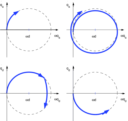
Figure 17: Scheme of quasiclassical matching, a-mode and b-mode phase-space wavepacket center trajectories for acceptor potential; Left panels illustrate reference wavepacket Eq. 38, a-mode: $\alpha=\delta\left(1+e^{-i\omega(t_{p}+t_{w})}\right)$ (upper panel), b-mode: $\beta=\delta\left(1+e^{i\omega t_{d}}\right)$ (lowe panel), dashed circles symbolize Franck-Condon Energy shell; Right panels illustrate target wavepacket Eq. 37 a-mode: $\alpha=\delta\left(e^{-i\omega\tau_{\cal A}}-1\right)e^{-i\omega t_{w}}$ (upper panel), b-mode: $\beta=\delta\left(1-e^{i\omega(\tau_{\cal A}-t_{w})}\right)$ (lowe panel); two arrows on lower panel symbolize the wavepacket center motion before (first arrow) and after (second arrow) the instant of transfer.

determine the mean position and momentum of the coherent state. Depending on the electronic state $\left\langle j\right|$ the mean values $\alpha(t)$, $\beta(t)$ circle around the minimum of the relevant harmonic potential surface: $(0,0)$ for $\left|0\right\rangle$, $(\delta,0)$ for $\left|1\right\rangle$, $(0,\delta)$ for $\left|1^{\prime}\right\rangle$, and $(\delta,\delta)$ for $\left|2\right\rangle$. Since $t_{p}$, $t_{w}$, $t_{d}$ are chosen one may follow the phase-space trajectories of $\alpha$, $\beta$ for target and reference states as shown in Fig. 17. In contrast to the reference wavefunction being always in either one of electronic states the target wavepacket reflects the dynamical entanglement formation between $|1>$, $|1^{\prime}>$, and nuclear modes. We specialize $t_{w}$ equal to half of vibrational period $\tau_{\rm vib}=2\pi/w$ to prevent multiple acts of the transfer. Target wavepacket evolves during the $t_{w}$ as discussed in section III.1. Initially it is nothing but coherent excitation in donor surface starting in position $(q_{a}=0,q_{b}=0)$ and oscillating about $(q_{a}=0,q_{b}=d)$.

Here we refer to the new variable ${\cal A}$ so that after ${\cal A}t_{w}$ time interval after $B_{x}$ pulse the first elementary act of transfer takes place. The variable ${\cal A}$ accounts for this moment of time only approximately and depend on energy arrangement of the potentials $E_{DA}=\epsilon_{1}-\epsilon_{1^{\prime}}$. The actual transfer is not instantaneous but continuos. After the act the transferred portion of the wavepacket amplitude does maintain its mean position and momentum, but starts to evolve about the minimum of the acceptor parabola (amplitudes in the basis of ground state potential). After it evolves in such a manner during the $(1-{\cal A})t_{w}$ time its position and momentum need to coincide with mean position and momentum of the reference wavepacket. The analytical condition of such coincidence reads

$$a-mode:(e^{i\omega{\cal A}t_{w}}-1)e^{-iwt_{w}}-1 = -e^{i\omega t_{d}},$$

$$b-mode:e^{-iw([1-{\cal A}]t_{w}+t_{d})} = e^{-iw(t_{p}+t_{w}+t_{d})}.$$ (41)

As far as $t_{w}$ is strictly fixed to be $\tau_{\rm vib}/2$ the conditions Eqs. 41 can be considered as system of two algebraic equations in respect to two variables $t_{p}$ and $t_{d}$. The solution of this equation gives the estimation when the target and reference wavepackets do overlap at best:

$$t_{p} = \left(m+1-{\cal A}/2\right)\tau_{\rm vib},$$

$$t_{d} = \left(n+{\cal A}/2\right)\tau_{\rm vib}.$$ (42)

It is integer multiples of vibrational period shifted far off resonance in the direction of smaller $t_{p}$ and larger $t_{d}$. ${\cal A}\simeq 0$ is expacted to be a bit larger than zero for equal site energies and ${\cal A}\simeq 1/4$ for the activationless downhill transfer. This analythis goes along with the results of the numerical simulations.

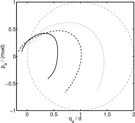
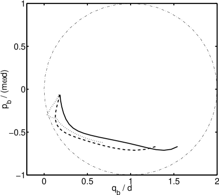
Figure 18: Calculated phase space trajectories for target wavepacket for $\epsilon_{1}-\epsilon_{1^{\prime}}=0$ (solid), $\epsilon_{1}-\epsilon_{1^{\prime}}=E_{\rm FC}$ (dashed), $\epsilon_{1}-\epsilon_{1^{\prime}}=2E_{\rm FC}$ (dotted); during the time interval $0<\omega t<\pi$, dot-dashed line points quasiclassical phase space trajectory in dispalced harmonic potential (Franck-Condon energy shell)

The calculated phase-space trajectories for target state are shown in Fig. 18. Starting and end points do not stay on the quasiclassical trajectory (on the FC energy shell). However, increase of site-energy difference shifts the trajectory end further (closer) from $(0,0)$ point in a-mode (b-mode).

V.4 Fringes

Figures 15, 16 also display fringes in target nuclear wavepackets. The maximal coincidence of target nuclear wavepacket with referrence wavepacket is one probable reason of the interferogram fringe structure. As long as interference structure is arranged to have no fringes along the line $t_{p}=t_{d}$ but change the sign along the line $t_{p}=-t_{d}$ the following speculations can be suitable: Change of the net signal phase of the phase-locking factor $\exp-i|\omega_{lock}(t_{p}-t_{d})$ takes place along the line $t_{p}-t_{d}$. This factor is zero for $t_{p}=t_{d}$ (and constant for $t_{p}=t_{d}+x$). In case there is an inhomogeneity between different dimers that form the sample, this factor will still have maximal value for $t_{p}=t_{d}$. This situation is analogeous to the stimulated photon echo scenario where the last pulse just plays the role of probe in order to detect the created net growth of the transition dipole moment mean value (homodyne detection).

Fringes in signals reflect (i) matching / mismatching of phase (ii) frequency of signal oscillations along $t_{p}$ and $t_{d}$ Information from fringe structure: Fringes Frequency corresponds to the mismatch of energy configuration and locking frequency. The difference of continuous and instantaneous transfer. An alternative interpretation rests on the velocity of the vavepacket.

TABLE 1. Position of signal amplitude maximum and rate of its phase change taken at the point of maximal signal amplitude.

configuration	$\frac{t_{\rm p}}{\tau_{\rm vib}}$	$\frac{t_{\rm d}}{\tau_{\rm vib}}$	$\frac{{\Gamma^{\prime}}_{t_{\rm p}}}{\omega}$	$\frac{{\Gamma^{\prime}}_{t_{\rm d}}}{\omega}$
equal $\epsilon_{1}-\epsilon_{1^{\prime}}=0$, quantum	$0.923$	$1.077$	$-0.53+i0.01$	$0.53-i0.01$
equal $\epsilon_{1}-\epsilon_{1^{\prime}}=0$, semiclassical	$1.000$	$1.000$	$0$	$0$
downhill $\epsilon_{1}-\epsilon_{1^{\prime}}=2E_{\rm FC}$, quantum	$0.750$	$1.250$	$-7.52+i0.01$	$0.13+i0.01$
downhill downhill $\epsilon_{1}-\epsilon_{1^{\prime}}=2E_{\rm FC}$, semiclassical	$0.750$	$1.250$	$-7.39$	$0$

VI Conclusions

We investigated the dynamical entanglement formation in a simple dimer with two nuclear modes energy transfer model system and its reflection by means of ultrafast nonlinear phase-locked wavepacket interferometry. We have revealed some intriguing features that may attract an attention of physical chemistry and quantum optics communities.

Following the ultrafast excitation of donor the population of acceptor state gets rised by small increments once per vibrational period. The long-time population oscillations between donor and acceptor states display collapses and revivals similar to those in Jaynes-Cummings model. The mean coordinate of the acceptor wavepacket loses its amplitude with time.

The intensity of the transfer is found to grow with depth of donor wavepacket penetration into the acceptor region. This depth depends on site-energy difference of donor and acceptor and amount of vibrational energy in donor potential in the transfer direction (perpendicular mode). The minor influence on the transfer intensity comes from initial phase of donor vibrational coherence and amount of vibrational energy in the parallel mode.

The consideration of the four-pulse phase-locked nonlinear wavepacket interferometry experiment on such model dimer shows that dimers with different site-energy difference provide different nonlinear optical response. The nonlinear wavepacket interferograms corresponding to equal-site energy dimer and activationless dimer have maxima at different delays between excitation pulses. This difference is predicted with satisfactory precision using quasiclassical analysis of the wavepacket mean trajectories.

The possible future development of this research should include the consideration of disoriented sample. Further work will account for vibrational relaxation and inhomogeneity of site energies and dipole-dipole coupling induced by various spatial orientations and distances between monomers, as well as application of these findings to the real molecular aggregate.

Acknowlegement

The research was supported by NSF, CAREER Award CHE-0094012. OVP is a Camille and Henry Dreyfus New Faculty and an Alfred P. Sloan Fellow. DSK thanks Howard Carmichael, Levente Horvath, and Jens Noeckel for useful comments and fruitful discussions.

Figure 14: Double-side Feynmann diagram, reprsenting processes contributing to interference population $P_{1\prime}=<0|A^{\dagger}_{\rm y}|\times|D_{\rm x}C_{\rm x}B_{\rm x}|0>$; left part symbolizes ket-vector $|D_{\rm x}C_{\rm x}B_{\rm x}|0>$; right part symbolizes bra-vector $<0|A^{\dagger}_{\rm y}|$; straight arrowed line stands for time evolution of a single chromophore (two-level-system); wiggly line stands for acquanted (tail down) or emitted (tail up) photon; doubly wiggly line stands for exciton transfer between chromophores.

References

- [1] T. S. Humble, J. A. Cina, Phys. Rev. Lett. 93 060402 (2004).
- [2] H. van Amerongen, L. Valkunas, and R. van Grondelle, Photosynthetic Excitons, (World Scientific, Singapore, 2000).
- [3] E. I. Zenkevich, A. Willert, S. M. Bachilo, U. Rempel, D. S. Kilin, A. M. Shulga, C. von Borczyskowski, Materials Sci. Eng. C, 18 99 (2001); E. I. Zenkevich, D. S. Kilin, A. Willert, S. M. Bachilo, A. M. Shulga, U. Remel, C. v. Borczyskowski, Mol. Cryst. Liq. Cryst. 361 83 (2001).
- [4] J-aggregates, ed. T. Kobayashi (World Scientific, Singapore, 1996)
- [5] Th. Förster, in: Modern Quantum Chemistry, ed. O. Sinanoglu, Ed., (Academic , NY, 1965)
- [6] G. Juzeliunas and J. Knoester J. Chem. Phys., 112 2325 (2000).
- [7] M. Yang and G. R. Fleming Chem. Phys., 275 335 (2002).
- [8] P. Reineker, in: G. Hohler (ed.), Exciton dynamics in molecular crystalls and aggregates, Springer Tracts Mod. Phys., 94 111 (1982).
- [9] E. O. Potma and D. A. Wiersma, J. Chem. Phys., 108 4894 (1998).
- [10] A. M. King, D. Bingemann, and F. F. Crim, J. Chem. Phys., 113 5018 (2000).
- [11] A. Matro and J. A. Cina J. Phys. Chem., 99 2568, (1995).
- [12] R. Jimenez, S N. Dikshit, S. E. Bradforth, and Graham R. Fleming. J. Phys. Chem., 100 6825, (1996).
- [13] K. Misawa and T. Kobayashi, J. Chem. Phys., 110 5894 (1999).
- [14] J. Moll, W. J. Harrison, D. V. Brumbaugh, and A. A. Muenter, J. Phys. Chem. A, 104 8847 (2000).
- [15] I. Yamazaki, S. Akimoto, T. Yamazaki, S. Sato, and Y. Sakata.J. Phys. Chem. A, 106 2122, (2002).
- [16] A. H. Zewail. J. Phys. Chem. A, 104 5660 (2000).
- [17] N. F. Scherer, R. Carlson, A. Matro, M. Du, A. J. Ruggiero, V. Romero-Rochin, J. A. Cina, G. R. Fleming, and S. A. Rice, J. Chem. Phys., 95 1487 (1991).
- [18] N. F. Scherer, R. Carlson, A. Matro, M. Du, L. D. Ziegler, J. A. Cina, and G. R. Fleming, J. Chem. Phys., 96 4180 (1992).
- [19] J. A. Cina, D. S. Kilin, T. S. Humble, J. Chem. Phys. 118 46 (2003).
- [20] J. A. Cina, G. R. Fleming, J. Phys. Chem. A 108 11196 (2004).
- [21] B. M. Garraway and N. V. Vitanov, Phys. Rev. A, 55 4418 (1997).
- [22] I. I. Rabi. Phys. Rev., 51 652 (1937).
- [23] F. Bloch, Phys. Rev., 70 460 (1946).
- [24] S. Mukamel, Principles of Nonlinear Optical Spectroscopy, (Oxford, 1999).
- [25] L. Allen and J. H. Eberly, Optical Resonance and Two-Level Atoms (Wiley-VCH, 1975).
- [26] E. T. Jaynes and F. W. Cummings, Proc. IEEE, 51 89 (1963).
- [27] M. Nakano and K. Yamaguchi, J. Chem. Phys. 116, 10069 (2002); ibid 117 9671 (2002).
- [28] J. A. Cina, J. Raman Spectroscopy, 31 1 (2000).
- [29] L. D. Landau, Phys. Z. Sowjetunion, 2 46, (1932).
- [30] N. Rosen and C. Zener. Phys. Rev., 40 502, (1932).
- [31] R. Marcus. J. Electroanal. Chem., 438 251, (1997); R. A. Marcus, J. Chem. Phys. 24, 966 (1956); Rev. Mod. Phys. 65, 599 (1993); R. A. Marcus and N. Sutin, Biochim. Biophys. Acta 811, 265 (1985).
- [32] M. Schreiber, D. Kilin, and U. Kleinekathöfer, J. Lumin. 83&84, 235 (1999).
- [33] V. May and O. Kühn, Charge and Energy Transfer Dynamics in Molecular Systems, (Wiley-VCH, 2000).
- [34] G. C. Schatz and M. A. Ratner, Quantum mechanics in chemistry, (Englewood Cliffs, NJ, Prentice Hall, 1993).
- [35] C. Fuchs and M. Schreiber. J. Chem. Phys., 105 1023, (1996).
- [36] T. Mancal, G. R. Fleming, J. Chem. Phys. 121 10556 (2004).
- [37] J. A. Cina, D. S. Kilin, T. S. Humble, J. Chem. Phys. 118 46 (2003).
- [38] D. Jonas, Ann. Rew. Phys. Chem. 54 425 (2003).
- [39] M. Weissbluth. Photon-Atom Interactions, Academic, (1989).