Measurement of geometric phase for mixed states using single photon interferometry
Abstract
Geometric phase may enable inherently fault-tolerant quantum computation. However, due to potential decoherence effects, it is important to understand how such phases arise for mixed input states. We report the first experiment to measure mixed-state geometric phases in optics, using a Mach-Zehnder interferometer, and polarization mixed states that are produced in two different ways: decohering pure states with birefringent elements; and producing a nonmaximally entangled state of two photons and tracing over one of them, a form of remote state preparation.
pacs:
03.65.Vf, 03.67.Lx, 42.65.LmWhen a pure quantum state undergoes a cyclic progression, besides the dynamical phase which depends on the evolution Hamiltonian, it retains memory of its motion in the form of a purely geometric phase factor Panchar56 ; Ber84 . This pure-state geometric phase has been experimentally demonstrated in various systems such as single photon interferometry Kwiat91 , two-photon interferometry twophotonphase , and NMR Suter88 . Recently, it has been proposed that fault-tolerant quantum computation may be performed using geometric phases geomet , since they are independent of the speed of the quantum gate and depend only on the area of the path the state takes in Hilbert space. The next step is to investigate the resilience of geometric phases to decoherence, and for this a well defined notion of a mixed state geometric phase is needed. Some properties of geometric phases for mixed states, proposed by Sjöqvist et al. sjoqvist , have been recently investigated in NMR Du03 . Here, we report the first experimental study of geometric phase for mixed quantum states with single photons. Due to the exquisite control achievable with optical qubits, we precisely map the behavior of the phase for various amounts of mixture, yielding experimental data in very good agreement with theoretical predictions. These results are particularly encouraging in light of recent work on scalable linear optics quantum computation klm .
In order to measure a geometric phase, the dynamical phase has to be eliminated. It can either be canceled, for example, using spin-echo technique for spins in magnetic fields Ekert00 , or one can parallel transport the state vector in order to ensure that the dynamical phase is zero at all times. The parallel transport condition for a particular state vector is , which implies that there is no change in phase when evolves to , for some infinitesimal change in time . However, even though the state does not acquire a phase locally, it can acquire a phase globally after completing a cyclic evolution. This global phase is equal to the geometric phase, and has its origin in the underlying curvature of the state space. It is therefore resilient to certain dynamical perturbations of the evolution, e.g., it is independent of the speed (or acceleration) of evolution.
Uhlmann uhlmann was the first to describe mixed-state geometric phases in a mathematical context where the parallel transport of a mixed state is defined in a larger state space which purifies the mixed state purify . In this approach the number of parallel transport conditions for a known density matrix is , but the time evolution operator of such a density matrix has only free variables. This approach can only be described in a larger Hilbert space with the system and an attached ancilla evolving together in a parallel manner EPSBO2002 .
Sjöqvist et al. defined a mixed-state geometric phase where no auxiliary subsystem is needed sjoqvist ; EPSBO2002 . This phase can be investigated using an interferometer in which a mixed state is parallel transported by a unitary operator in one arm; the output then interferes with the other arm, which has no geometric phase. The parallel transport of a mixed state is given by i.e., each eigenvector of the initial density matrix is parallel transported by the unitary operator. The resulting conditions uniquely determine the unitary operator and ensure the gauge invariance of the geometric phase. One consequence of invariance is that each eigenvector acquires a geometric phase , and an associated interference visibility . The total mixed-state geometric phase factor is then obtained as an average of the individual phase factors, weighted by :
| (1) |
The polarization mixed state of a single photon can be represented by its density operator, which can be written in terms of the Bloch vector and the Pauli matrices , as . It represents a mixture of its two eigenvectors with eigenvalues . The length of the Bloch vector gives the measure of the purity of the state, from completely mixed () to pure (). For photons of purity , Eq. (1) becomes
| (2) |
where is the solid angle enclosed by the trajectory of one of the eigenvectors on the Bloch sphere with corresponding geometric phase (the other eigenvector traverses the same trajectory, but in the opposite direction, leading to a geometric phase ). From Eq. (2) we obtain the visibility and geometric phase, respectively, sjoqvist
| (3) | |||||
| (4) |
Here is measured in an interferometer by plotting the output intensity versus an applied dynamical phase shift in one interferometer arm. For pure states, the geometric phase given by (4) reduces to half the solid angle ().
In our experiment, single-photon states are conditionally produced by detecting one member of a photon pair produced in spontaneous parametric downconversion (SPDC) hong (we also took data using coherent states from a diode laser). Specifically, pairs of photons at 670 nm and the conjugate wavelength 737 nm are produced via SPDC by pumping Type-I phase matched BBO with an Ar+ laser at nm. By conditioning on detection of a 737-nm “trigger” photon (with an avalanche photodiode after a 5-nm FWHM interference filter at 737 nm), the quantum state of the conjugate mode is prepared into an excellent approximation of a single-photon Fock state at 670 nm Kwiat91 ; hong , also with wavelength spread nm. As shown in Fig. 1, the 670-nm photons are coupled into a single-mode optical fiber to guarantee a single spatial mode input for the subsequent interferometer. A fiber polarization controller is used to cancel any polarization transformations in the fiber.
The mixedness of the -nm photons is set via two different methods KE . The first uses thick birefringent decoherers that couple the single photon’s polarization to its arrival time relative to the trigger berglund ; footnote:laser . Consider a horizontally polarized () and a vertically polarized () photon. Assuming the decoherers delay vertically polarized photons relative to horizontally polarized photons by more than the photon’s coherence length (given by ), upon detection of the trigger photon, will in principle be detected before . Tracing over the timing information during state detection erases coherence between these distinguishable states; this is equivalent to irreversible decoherence KE .
To guarantee a pure fiducial state for this method of generating mixed states, a horizontal polarizer is placed after the polarization controller, followed by a half-waveplate (HWP), and finally the decoherers (four pieces of quartz of 3 cm total thickness). By rotating the HWP, the state can be prepared in an arbitrary superposition . The light is then sent through the decoherers, effectively erasing the off-diagonal terms in the density matrix, resulting in purity . In our experiment, the eigenstates of the net geometric phase operator are circular polarizations; therefore, before entering the interferometer, the quantum state is rotated with a quarter-waveplate (QWP) into a mixture of left () and right () circular polarized light.
Our second method to produce mixed-polarization single-photon states, a version of remote state preparation bennett01 , is to trace over one of the photons of a pair initially in a nonmaximally entangled polarization state. This state is prepared using two thin BBO crystals oriented such that pumping with polarization produces a variable entanglement superposition state Kwiat99 . Here, the first position polarization label corresponds to the trigger photon (at 737 nm) while the second corresponds to its partner (at 670 nm). A polarization-insensitive measurement of the trigger photon prepares the partner in the polarization mixed state , with . is then transported over the single-mode fiber (still with the polarization controller so the fiber does not alter the state). As before, a QWP is used to rotate the photon’s polarization state to a mixture of and before entering the interferometer.
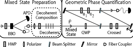
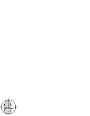
After any of the above mixed state preparations, the photon is sent into a Mach-Zehnder interferometer (Fig. 1). In the upper arm, the Bloch vector is evolved unitarily using two half-waveplates with optic axes at and , respectively. The evolution can be illustrated (Fig. 2) with one of the eigenvectors of the density matrix, e.g., , traveling along two geodesics going from to and back. The trajectory encloses a solid angle footnote:wps . The other eigenvector takes the same path but in the opposite direction, and therefore encloses the solid angle . For mixed states, the length of is reduced, but the same solid angle is subtended. The resulting evolution fulfills the parallel transport conditions for mixed states, and the induced geometric phase is obtained by substituting into equations (3) and (4). A motorized rotation stage is used to set (to within ) and thus, the geometric phase.
To measure and , we apply a dynamical phase shift in the lower interferometer arm and measure the resulting interference pattern both with a geometric phase (for several settings of footnote:wedge ) and without (). The dynamical phase shift is produced with a piezoelectric transducer (PZT) on the translation stage on which the lower path mirror is mounted. By adjusting the voltage across the PZT, the length difference () between the arms is varied, giving the probability for the photon to exit the interferometer to the detector as
| (5) |
Photons are detected using an avalanche photodiode. To conditionally prepare a single-photon Fock state with the desired bandwidth, we count only coincident detections (within a 4.5-ns timing window) with the trigger detector. We estimate the probability of two photons being present accidentally during a given coincidence window is for the decoherer method (using a 4-mm thick BBO crystal) and for the entanglement method (using two 0.6-mm crystals). Thus the “accidental” coincidence rate (e.g., between photons corresponding to different pairs, or from detector dark counts) is negligible, and has not been subtracted from the data.
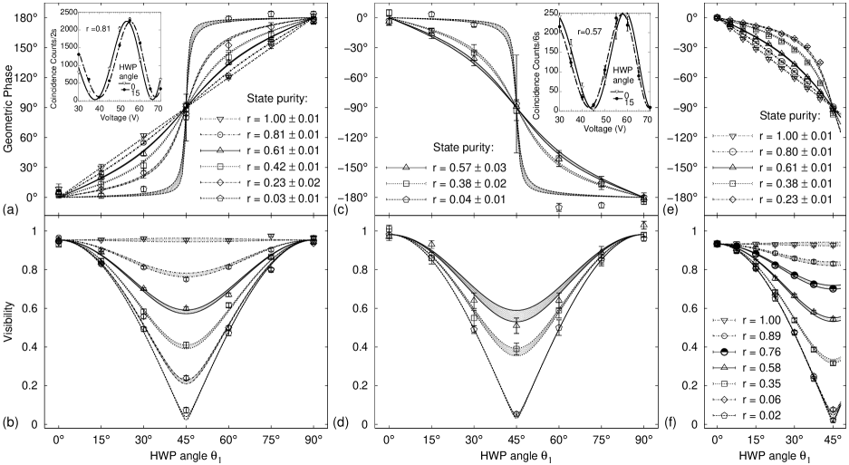
Data is taken by varying the PZT voltage from to volts, in volt steps, giving slightly more than one period of the interference pattern. At each voltage, data is accumulated for s (decoherer method) or 6 s (traced-over entangled state method). We plot the number of coincidences as a function of PZT voltage, and then fit a curve to extract the phase and visibility information for each HWP setting footnote:volt . To calculate the phase difference due to the geometric phase, we relate the data for each HWP setting to the reference data with (see inset in Figs. 3(a) and 3(c)) footnote:averages .
The experimental data are plotted in Figs. 3(a)-3(f), along with theoretical curves based on the measured purity of the photons. To determine the purity, we measure the and components of the mixed state before the last quarter-waveplate in front of the interferometer. Figs. 3(a)-(b) show the data for the geometric phase and the visibility, respectively, for the experiment where the single photons are decohered with thick birefringent quartz. Figs. 3(c)-3(d) show the corresponding data when the mixture is due to entanglement to the trigger photon. Figs. 3(e)-3(f) show results from the coherent state, indicating that the data clearly fits the theoretical prediction and demonstrates that the single-photon geometric phase survives the correspondence principle classical limit Kwiat91 . The two geometric phase plots, Fig. 3(a) and Fig. 3(c) are flipped along the axis: in the first setup the input states possessed larger right-circular polarization eigenvalues, while in the second setup, left-circular polarization was dominant footnote:flip .
Fig. 3’s error bars arise from the fitting program’s uncertainty estimate of the phase and visibility from the raw fringes. This error is consistent with the standard error obtained from repeating measurements four times to calculate the spread in the geometric phase and visibility. We quantify how well the data fits the theory using a weighted reduced -analysis. For the geometric phases (visibilities), we obtain average values of 0.98 (1.36) and 1.14 (0.94) for the decoherer and entangled state preparations, respectively, indicating an excellent fit. Also, the values of retrodicted from our fringe data agree with our direct measurements of within uncertainty.
We report the first measurement of geometric phases for single photons prepared in various polarization mixed states, created using two different methods. Specifically, we report a novel way of creating decohered one-qubit states from entangled two-qubit states, a simple version of remote state preparation. Both types of mixed states give geometric phase and visibility data in very good agreement with the theoretical predictions. Given the recent advances in linear optical quantum computation klm , and continued interest in geometric quantum computation geomet , our results indicate that we have a good measure of the geometric phase for mixed states, which in future work will enable the estimation of fault tolerance in geometric quantum computation with linear optical elements. We also anticipate further experiments on non-unitarily evolved mixed states EPSBO2002 and non-Abelian geometric phases wilczek84 , to ultimately realize a universal set of geometric gates for quantum computation pachos .
We thank J. B. Altepeter, E. R. Jeffrey, A. VanDevender, and T.-C. Wei for valuable discussions and technical assistance. M.E. acknowledges financial support from The Foundation BLANCEFLORBoncompagni-Ludovisi, ne Bildt. We recognize partial support from the National Science Foundation (Grant #EIA-0121568).
References
- (1) Present address: Dept. of Physics and Optical Eng., Rose-Hulman Inst. of Tech., Terre Haute, Indiana, 47803.
- (2) S. Pancharatnam, Proc. Ind. Acad. Sci. A 44, 247 (1956).
- (3) M. V. Berry, Proc. Roy. Soc. A 392, 45 (1984).
- (4) P. G. Kwiat and R. Y. Chiao, Phys. Rev. Lett. 66, 588 (1991).
- (5) J. Brendel, W. Dultz, and W. Martienssen, Phys. Rev. A 52, 2551 (1995); D. V. Strekalov and Y. H. Shih, Phys. Rev. A 56, 3129 (1997).
- (6) D. Suter, K. T. Mueller, and A. Pines, Phys. Rev. Lett. 60, 1218 (1988).
- (7) J. A. Jones et al.,Nature 403, 869 (2000); P. Zanardi and M. Rasetti, Phys. Lett. A 264, 94 (1999); L. M. Duan, J. I. Cirac, and P. Zoller, Science 292, 1695 (2001); S.-L. Zhu and Z. D. Wang, Phys. Rev. Lett. 91, 187902 (2003).
- (8) E. Sjöqvist et al., Phys. Rev. Lett. 85, 2845 (2000).
- (9) J. Du et al., Phys. Rev. Lett. 91, 100403 (2003).
- (10) E. Knill, R. Laflamme, and G. Milburn, Nature 409, 46 (2001); T. B. Pittman, B. C. Jacobs, and J. D. Franson, Phys. Rev. Lett. 88, 257902 (2002); T. B. Pittman et al., Phys. Rev. A 68, 032316 (2003); J. L. O’Brien et al., Nature 426, 264 (2003).
- (11) A. Ekert et al., J. Mod. Opt. 47, 2501 (2000).
- (12) A. Uhlmann, Rep. Math. Phys. 24, 229 (1986).
- (13) M. A. Nielsen and I. L. Chuang, Quantum Computation and Quantum Information (Cambridge University Press, Cambridge, 2000), pp. 109-111.
- (14) M. Ericsson et al., Phys. Rev. Lett. 91, 090405 (2003).
- (15) C. K. Hong and L. Mandel, Phys. Rev. Lett. 56, 58 (1986).
- (16) P. G. Kwiat and B.-G. Englert, in Science and Ultimate Reality: Quantum Theory, Cosmology and Complexity, J. D. Barrow, P. C. W. Davies, and C. L. Harper, Jr., Eds., Cambridge Univ. Press (2004).
- (17) A. J. Berglund, Dartmouth College B.A. Thesis, also quant-ph/0010001 (2000); N. Peters et al., Quant. Inf. Comp. 3, 503 (2003).
- (18) The classical light is similarly mixed, using an unbalanced polarizing interferometer to separate and by more than the 1 m diode laser coherence length.
- (19) C. H. Bennett et al., Phys. Rev. Lett. 87, 077902 (2001).
- (20) P. G. Kwiat et al., Phys. Rev. A 60, R773 (1999).
- (21) We can fix , since depends only on .
- (22) The adjustable waveplate must not be wedged, or the path overlap will be ruined when the waveplate is rotated.
- (23) Because the voltage applied to the PZT creates a nonlinear increase in the path length, we fit our data to a sinusoid with nonlinear dependence on the argument. The PZT nonlinear fit parameters were determined by measuring dynamical phase fringes in our interferometer.
- (24) To reduce the effect of dynamical phase drift, the reference data is taken both before and after each geometric phase-generating HWP setting. The data for each specific waveplate setting is used to calculate the geometric phase relative to both the initial and final reference data; the reported result is the average of the two calculations.
- (25) The initial state was prepared more right circular polarized than left, opposite of the initial states for the and trials. Therefore, for ease of comparison with these curves, the data curve is displayed flipped about the horizontal.
- (26) F. Wilczek and A. Zee, Phys. Rev. Lett. 52, 2111 (1984).
- (27) J. Pachos, P. Zanardi, and M. Rasetti, Phys. Rev. A 61, 010305(R) (1999).