Decoherence induced by zero point fluctuations in quantum Brownian motion

Abstract

We show a completely analytical approach to the decoherence induced by a zero temperature environment on a Brownian test particle. We consider an Omhic environment bilinearly coupled to an oscillator and compute the master equation. From diffusive coefficients, we evaluate the decoherence time for the usual quantum Brownian motion and also for an upside-down oscillator, as a toy model of a quantum phase transition.

I Introduction

The emergence of classical behavior from a quantum system is a problem of interest in many branches of physics giul . As it is well known, the quantum to classical transition involves two necessary and related conditions: correlations, i.e. the Wigner function of a quantum system should have a peak at the classical trajectories; and decoherence, that is, there should be no interference between classical trajectories. To study quantitatively the emergence of classicality, it is essential to consider the interaction of the system with its environment, since both, the loss of quantum coherence and the onset of classical correlations, depend strongly on this interaction unruhzu . Using this point of view, classicality is an emergent property of an open quantum system. The strength of the coupling between system and environment sets the decoherence time which, roughly speaking, indicates the timescale after which the system can be considered classical zurek .

The very notion of quantum open system implies the appearance of dissipation and decoherence as an ubiquitous phenomena and plays important roles in different branches of physics (from quantum field theory, many body and molecular physics to theory of quantum information), biology and chemistry. Oftentimes, a large system can be described adequately as a composite system, consisting of two or a few subsystems (degrees of freedom) interacting with their environment (thermal bath) comprising a large number of degrees of freedom. Examples include electron transfer in solution, large biological molecules, vibrational relaxation of molecules in solution, excitons in semiconductors coupled to acoustic or optical phonon modes. Quantum processes in condensed phases are usually studied by focusing on a small subset of degrees of freedom and treating the rest as a bath.

Decoherence is the main ingredient in order to find classicality. The interaction between the system and the environment induces a preferred basis which is stable against this interaction, and becomes a classical basis in the Hilbert space of the coupled system. Preferred pointer states are resilient to the entangling interaction with the bath. This “einselection” (environment induced superselection) of the preferred set of resilient pointer states is the essence of the environment. It is accepted that a rapid loss of coherence caused by the coupling with the environment is at the root of the non-observation of quantum superpositions of macroscopically different quantun states zurek . A relevant property of the pointer states is their insensitivity to being monitored by the interaction with environment (and, therefore, are resistant to the entanglement caused by the environment). The less the states entangle, the more stable they are. All other states evolve into joint system-environment states, preserving their purity.

Our concern in this Letter is to analyze the effect of the zero point fluctuations of the environment, as a source of decoherence. The coupling of a quantum system to an environment generally leads to energy fluctuations in the test particle even at zero temperature nagaevEPL . Since phases are time integrals of energy, zero point energy fluctuations make possible that decoherence occurs even at zero temperature. These fluctuations are a consequence of the finite coupling energy between the test particle (system) and the bath, and of the fact that the Halmiltonian of the isolated system does not commute with the interaction Hamiltonian.

Vacuum fluctuations have several observable effects. The Lamb shift is a widely known example. Another one is the Casimir effect. In these examples the effect of vacuum can be thought in terms of the renormalization of the original parameters characterizing the system. In contrast, the fluctuations we deal with in this Letter are not only absorbed into renormalized parameters of the test particle. Not only does the environment renormalize, but also it is a source of dissipation and noise for the system. Therefore, we are considering the effect of quantum fluctuations of the environment over a quantum system, as the only source of decoherence (meaning that there is no possible thermal fluctuations inducing classicality).

The question about the influence of zero temperature environment on the interference phenomena has been discussed in the last years ford ; imry ; sinha . There have been studies on the temperature dependent weak localization measurements 4ratchov , reporting residual decoherence in metals at zero temperature, in contradiction to theoretical predictions 5ratchov , and on the zero-point decoherence induced by Coulomb interactions in disordered electron systems; just to mention a few examples.

In previous works (see for example leshouches for an excellent review of the state of the art of decoherence) about decoherence in quantum Brownian motion, most of the conclusions are simply numerical or analytical only in the high temperature limit jpphabzurek . Low temperature case was discussed in leshouches ; jppdavila showing a numerical estimation of the decoherence rate. S. Sinha, in Ref. sinha , studied the zero temperature case analytically. Under some approximations the author found an expression for the time dependence of the off-diagonal terms of the density matrix. In this Letter, we complete that study showing an exact calculation of diffusive terms, and also providing the decoherence timescale for different situations of interest. In addition, we solve the master equation for an upside-down Brownian particle to emphasize the role of zero temperature fluctuations during a second order phase transition guthpi ; order .

II The master equation at T=0

Let us consider a quantum particle (characterized by its mass $M$ and its bare frequency $\Omega$) linearly coupled to an environment composed of an infinite set of harmonic oscillators (of mass $m_{n}$ and frequency $\omega_{n}$). We may write the total action corresponding to the system-environment model as (we set $\hbar=1$)

$$S[x,q_{n}] = S[x]+S[q_{n}]+S_{\rm int}[x,q_{n}]$$ (1)

$$= \int_{0}^{t}ds\left[\frac{1}{2}M({\dot{x}}^{2}-\Omega^{2}x^{2})+\sum_{n}\frac{1}{2}m_{n}({\dot{q}}_{n}^{2}-\omega_{n}^{2}q_{n}^{2})\right]-\sum_{n}C_{n}xq_{n},$$

where $x$ and $q_{n}$ are the coordinates of the particle and the oscillators, respectively. The particle is coupled linearly to each oscillator with strength $C_{n}$.

The relevant objects to analyze the quantum to classical transition in this model are the reduced density matrix (obtained from the full density matrix integrating out all the degrees of freedom of the environment noted as ${\bar{q}}$), and the associated Wigner function

$$\rho_{\rm r}(x,x^{\prime},t) = \int d{\bar{q}}\,\,\rho(x,{\bar{q}},x^{\prime},{\bar{q}},t)$$

$$W_{\rm r}(x,p,t) = \frac{1}{2\pi}\int_{-\infty}^{+\infty}dy~{}e^{ipy}~{}\rho_{\rm r}(x+\frac{y}{2},x-\frac{y}{2},t).$$ (2)

The reduced density matrix satisfies a master equation. Hu-Paz-Zhang hpz have evaluated the master equation for the quantum Brownian motion problem (alternatively, one can write an equation of the Fokker-Planck type for the reduced Wigner function jpphabzurek in order to study the dynamics in phase space)

$$\dot{\rho}_{\rm r}=-i\bigl{[}{H}_{\rm syst}+\frac{1}{2}M{\tilde{\Omega}}^{2}x^{2},\rho_{\rm r}\bigr{]}-i\gamma(t)\bigl{[}x,\bigl{\{}p,\rho_{\rm r}\bigr{\}}\bigr{]}-D(t)\bigl{[}x,\bigl{[}x,\rho_{\rm r}\bigr{]}\bigr{]}-f(t)\bigl{[}x,\bigl{[}p,\rho_{\rm r}\bigr{]}\bigr{]}.$$ (3)

The time dependent coefficients (in the case of weak coupling to the bath) are given by

$${\delta\Omega}^{2}(t) = -\frac{2}{M}\int_{0}^{t}ds\cos(\Omega s)\eta(s)$$

$$\gamma(t) = \frac{1}{M\Omega}\int_{0}^{t}ds\sin(\Omega s)\eta(s)$$

$$D(t) = \int_{0}^{t}ds\cos(\Omega s)\nu(s)$$ (4)

$$f(t) = -\frac{1}{M\Omega}\int_{0}^{t}ds\sin(\Omega s)\nu(s),$$

where ${\delta\Omega}^{2}(t)$ is the shift in frequency, which produces the renormalized frequency ${\tilde{\Omega}}^{2}$ that appears in the master equation. $\gamma(t)$ is the dissipation coefficient related to the friction kernel defined below, and $D(t)$ and $f(t)$ are the diffusion coefficients, which produce the decoherence effects. Diffusion coefficients come from the noise kernel, source of stochastic forces in the associated Langevin equation. $f(t)$ is named anomalous in the literature since it generates a second derivative term in the phase space representation of the evolution equation, just like the ordinary diffusion term unruhzu . $\eta(t)$ and $\nu(t)$ are the dissipation and noise kernels, respectively,

$$\eta(t) = \int_{0}^{\infty}d\omega I(\omega)\sin\omega t$$

$$\nu(t) = \int_{0}^{\infty}d\omega I(\omega)\coth\frac{\beta\omega}{2}\cos\omega t,$$

$I(\omega)$ is the spectral density of the environment, defined as $I(\omega)=(2/\pi)M\gamma_{0}\Lambda^{2}\omega/(\omega^{2}+\Lambda^{2})$ (where $\Lambda$ is the physical high-frequency cutoff, which represents the highest frequency present in the environmet). In the high temperature limit of an ohmic environment (where $I(\omega)\propto\omega$) the coefficients in Eq.(4) become constants. In particular, the diffusion coefficient can be approximated by $D\simeq 2\gamma_{0}k_{\rm B}TM$, where $\gamma_{0}$ is the dissipation coefficient hpz . In this limit, while $\gamma_{0}$ is a constant and $D\propto T$, the coefficient $f\propto T^{-1}$ can be neglected. Therefore, the term proportional to $D$ is the relevant one in the master equation at high temperatures in order to evaluate decoherence.

We will evaluate the time dependent coefficients of the master equation at zero temperature. For this, we set $\coth\beta\hbar\omega/2=1$. These coefficients have been evaluated previously in Refs.jppdavila ; vinales .

The shift in frequency ${\delta\Omega}^{2}(t)$ is,

$${\delta\Omega}^{2}(t)=-\frac{4\gamma_{0}}{\pi}\Lambda^{2}\int_{0}^{\infty}d\omega\int_{0}^{t}ds\frac{\omega}{\omega^{2}+\Lambda^{2}}\sin\omega s\cos\Omega s,$$ (5)

performing integrations, we obtain

$${\delta\Omega}^{2}(t)=-2\gamma_{0}\frac{\Lambda^{3}}{\Lambda^{2}+\Omega^{2}}\left[1-e^{-\Lambda t}\left(\cos\Omega t-\frac{\Omega}{\Lambda}\sin\Omega t\right)\right],$$ (6)

for times such that $\Lambda t>1$ the shift reads (see Fig. 1 (a))

$${\delta\Omega}^{2}=-2\gamma_{0}\frac{\Lambda^{3}}{\Lambda^{2}+\Omega^{2}}.$$ (7)

Dissipation coefficient (Fig. 1 (b)) comes from the integral

$$\gamma(t)=\frac{2\gamma_{0}}{\pi\Omega}\Lambda^{2}\int_{0}^{\infty}d\omega\int_{0}^{t}ds\frac{\omega}{\omega^{2}+\Lambda^{2}}\sin\omega s\sin\Omega s,$$ (8)

and it is given by

$$\gamma(t)=\gamma_{0}\frac{\Lambda^{2}}{\Lambda^{2}+\Omega^{2}}\left[1-e^{-\Lambda t}\left(\cos\Omega t+\frac{\Lambda}{\Omega}\sin\Omega t\right)\right],$$ (9)

which has the following asymptotic behavior

$$\gamma(t)=\gamma_{0}\frac{\Lambda^{2}}{\Lambda^{2}+\Omega^{2}}.$$ (10)

The normal diffusive coefficient (normally connected with decoherence effects) is coming from the integral

$$D(t)=\frac{2M\gamma_{0}}{\pi}\Lambda^{2}\int_{0}^{\infty}d\omega\int_{0}^{t}ds\frac{\omega}{\omega^{2}+\Lambda^{2}}\cos\omega s\cos\Omega s.$$ (11)

This integral can be exactly solved. The result is:

$$D(t) = \frac{2M\gamma_{0}}{\pi}\frac{\Lambda^{2}\Omega}{\Omega^{2}+\Lambda^{2}}\left[Shi(\Lambda t)\left(\frac{\Lambda}{\Omega}\cos\Omega t\cosh\Lambda t+\sin\Omega t\sinh\Lambda t\right)\right.$$ (12)

$$- \left.Chi(\Lambda t)\left(\frac{\Lambda}{\Omega}\cos\Omega t\sinh\Lambda t+\sin\Omega t\cosh\Lambda t\right)\right.$$

$$+ \left.Si(\Omega t)\right],$$

where, $Chi(x)$ and $Shi(x)$ are the hyperbolic CosIntegral and SinIntegral respectively; $Si(x)$ is the SinIntegral.

The expression can be very well approximated, when $\Lambda t>1$, by

$$D(t)=\frac{2M\gamma_{0}}{\pi}\frac{\Lambda^{2}\Omega}{\Omega^{2}+\Lambda^{2}}Si(\Omega t).$$ (13)

This coefficient is the normal diffusion at $T=0$. This is for any value of $\Omega$. We are interested in time scales longer than the memory time $1/\Lambda$. This coefficient is an oscillatory function of time. In fact, only in the limit $\Omega t\gg 1$, as $Si$ goes to $\pi/2$, we can have an asymptotic value $D_{\infty}\sim M\gamma_{0}\Lambda^{2}\Omega/(\Lambda^{2}+\Omega^{2})$, independent of time leshouches (Fig. 1 (e)). In any other case, the coefficient has an initial transient and approaches the asymptotic value $D_{\infty}$ as the $Si$ (see Fig. 1 (c)). It is important to note, that in the opposite case, when $\Omega t\ll 1$, normal diffusion is a linearly growing function of time, $D\sim 2M(\gamma_{0}/\pi)\Lambda^{2}\Omega^{2}t/(\Lambda^{2}+\Omega^{2})$, similar to the result obtained in Ref.sinha .

The anomalous diffusion coefficient is given by the integral

$$f(t)=\frac{2\gamma_{0}}{\pi\Omega}\Lambda^{2}\int_{0}^{\infty}d\omega\int_{0}^{t}ds\frac{\omega}{\omega^{2}+\Lambda^{2}}\cos\omega s\sin\Omega s.$$ (14)

It reads as

$$f(t) = 2\gamma_{0}\frac{\Lambda^{2}}{\Omega^{2}+\Lambda^{2}}\left[Shi(\Lambda t)\left(\frac{\Lambda}{\Omega}\sin\Omega t\cosh\Lambda t-\cos\Omega t\sinh\Lambda t\right)\right.$$ (15)

$$+ \left.Chi(\Lambda t)\left(-\frac{\Lambda}{\Omega}\sin\Omega t\sinh\Lambda t+\cos\Omega t\cosh\Lambda t\right)\right.$$

$$- \left.Ci(\Omega t)-\log\frac{\Lambda}{\Omega}\right].$$

Again, for $\Lambda t>1$, this coefficient can be written as (Fig. 1 (d))

$$f(t)=2\gamma_{0}\frac{\Lambda^{2}}{\Omega^{2}+\Lambda^{2}}\left(-Ci(\Omega t)-\log\frac{\Lambda}{\Omega}\right),$$ (16)

coefficient $f(t)$ also approaches an asymptotic value when $\Omega t\gg 1$, $f_{\infty}\sim-2\gamma_{0}(\Lambda^{2}/(\Lambda^{2}+\Omega^{2}))\log\Lambda/\Omega$ (Fig. 1 (f)); and it does to $f(t)\sim-2\gamma_{0}(\log\Lambda t+\Gamma)$, when $\Omega t\ll 1$ ($\Gamma$ is the EulerGamma number).

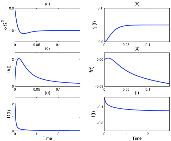
Figure 1: Time dependence of the coefficients of the master equation at $T=0$. On top we show frequency renormalization (a) and dissipation coefficients (b). Plots below show the normal $D$ (c) and anomalous $f$ (d) diffusion coefficients for short times in order to show the initial transient. Asymptotic values of diffusion are shown in (e) and (f). The parameters used in the plot are $\gamma_{0}=0.05$, $\Lambda=100$, $\Omega=1$.

In Fig. 1, we show the time behavior of these coefficients. It is easy to probe asymptotic behavior also from analytical expressions.

It has been noted that the master equation in the high temperature limit (or even in the $\gamma\sim$ constant approximation) has the pathology that the density matrix loses its positivity at short times (shorter than $1/k_{B}T$). This violation is essentially due to the action of the friction term. Master equation (3) does not have the pathological behaviour of the master equation at high temperature hpz . The dissipation coefficient is a time-dependent function that vanishes initially together with its first derivative. Therefore, the initial behaviour of the density matrix is diffusion dominated and positivity is preserved, even in the perturbative case, up to second order with respect to the coupling constant between system and environment.

With these coefficients at hand, we will evaluate the decoherence time following Refs.leshouches ; jpphabzurek .

III Decoherence time at T = 0

We will analyze the decoherence process in a simple case. We prepare an initial superposition of delocalized (in position or momentum) states. We consider two wave packets symmetrically located in phase space, of the form jpphabzurek : $\Psi(x,t=0)=\Psi_{1}(x)+\Psi_{2}(x)$, where

$$\Psi_{1,2}=N\exp\left(-\frac{(x\mp L_{0})^{2}}{2\delta^{2}}\right)\exp(\pm iP_{0}x),$$ (17)

$$N^{2}=\frac{{\tilde{N}}^{2}}{\pi\delta^{2}}=\frac{1}{2\pi\delta^{2}}\left[1+\exp\left(-\frac{L_{0}^{2}}{\delta^{2}}-\delta^{2}P_{0}^{2}\right)\right]^{-1},$$ (18)

where $N$ is normalization, and $\delta$ is the initial width of the wave packet. In terms of the Wigner function, the state at time $t$ is $W(x,p,t)=W_{1}(x,p,t)+W_{2}(x,p,t)+W_{\rm int}(x,p,t)$, where

$$W_{1,2}=\frac{{\tilde{N}}^{2}}{\pi}\frac{\delta_{1}}{\delta_{2}}\exp\left(-\frac{(x\mp x_{c})^{2}}{\delta_{1}^{2}}\right)\exp\left(-\delta_{2}^{2}(p\mp p_{c}-\beta(x\mp x_{c}))^{2}\right),$$ (19)

and

$$W_{\rm int}=\frac{2{\tilde{N}}^{2}}{\pi}\frac{\delta_{1}}{\delta_{2}}\delta_{2}^{2}(p-\beta x)^{2}\cos(2k_{p}p+2(k_{x}-\beta k_{p})x).$$ (20)

All the coefficients are functions of time, determined by the evolution propagator of the reduced density matrix and the initial state. The explicit form can be found in Ref. jpphabzurek . The initial state is such that $\delta_{1}^{2}=\delta_{2}^{2}=\delta^{2}$, $k_{x}=P_{0}=p_{c}$, $k_{p}=L_{0}=x_{c}$. $k_{p}$ and $k_{x}$ indicate the evolution of the fringes in the momentum and coordinates directions of the phase space.

As it was defined in the previous literature (see for example leshouches ), the effect of decoherence is produced by an exponential factor $\exp(-A_{\rm int})$, defined as

$$\exp(-A_{\rm int})=\frac{1}{2}\frac{W_{\rm int}(x,p)|_{\rm peak}}{\left[W_{1}(x,p)|_{\rm peak}W_{2}(x,p)|_{\rm peak}\right]^{\frac{1}{2}}}.$$ (21)

Initially, $A_{\rm int}=0$, and it is always bounded $A_{\rm int}\leq L_{0}^{2}/\delta^{2}+\delta^{2}P_{0}^{2}=A_{\rm int}|_{\rm max}$. The fringe visibility factor $A_{\rm int}$ evolves in time as ${\dot{A}}_{\rm int}=4D(t)k_{p}^{2}-4f(t)k_{p}(k_{x}-\beta k_{p})$. In the high temperature approximation, the anomalous coefficient is neglected and we obtain the very well known decoherence rate considering only the constant diffusion term, proportional to $T$. In our present case, at zero temperature, both coefficients $D$ and $f$ contribute to the fringe visibility factor. A conservative choice is to assume fringes always stay more or less frozen at the initial values, and we can set $k_{p}=L_{0}$ and $k_{x}=1/(2L_{0})$. Neglecting the initial transient (i.e. $\Lambda t>1$), we use Eqs.(13) and (16) to evaluate $A_{\rm int}$. In order to have the simplest analytical expression for the decoherence rate, we use a short time approximation to evaluate $\beta$, giving $\beta\sim 0$ (see jpphabzurek ). Thus, we get

$$\dot{A}_{\rm int}\approx 4L_{0}^{2}D(t)-2f(t).$$ (22)

In order to evaluate the decoherence time $t_{D}$, we have to solve $1\approx A_{\rm int}(t=t_{D})$. From Eq.(22) it is not possible to find a global decoherence time-scale at $T=0$. Nevertheless, we can find limits in which we are able to give different scales for decoherence.

For example, for large natural frequency $\Omega$, such as $\Omega\sim\Lambda$ ($\Omega t\gg 1$), it is easy to see that

$$A_{\rm int}\sim 2L_{0}^{2}M\gamma_{0}\Lambda t+4\gamma_{0}\left(t~{}Ci(\Lambda t)-\frac{\sin\Lambda t}{\Lambda}\right),$$ (23)

giving a very short decoherence time-scale,

$$t_{D}\sim\frac{1}{2ML_{0}^{2}\gamma_{0}\Lambda}.$$ (24)

This result will be valid as long as the product $ML_{0}^{2}\gamma_{0}\leq 1$, in order to be able to neglect the initial transient. It coincides with the decoherence time evaluated directly from $D_{\infty}$ as in Ref.leshouches . In this limit, the anomalous coefficient does not play any role (as we could check using $f_{\infty}$ in (24)).

In the opposite limit, when $\Omega t\ll 1$ (for times $\frac{1}{\Lambda}<t<\frac{1}{\Omega}$), we can approximate $A_{\rm int}$ using asymptotic limit of $Si$ and $Ci$ by

$$A_{\rm int}\approx\frac{8\Lambda^{2}}{\Lambda^{2}+\Omega^{2}}\gamma_{0}\left[\frac{ML_{0}^{2}}{2\pi}(\Omega t)^{2}+t~{}(\log\Lambda t+\Gamma-1)\right],$$ (25)

resulting in a decoherence time bound, $t_{D}\leq\frac{1}{8\gamma_{0}}$, which could be large for very underdamped systems. Here, the logarithmic correction is due to the $f(t)$ diffusion term (unlike Ref. sinha , where anomalous diffusion was neglected). This scale is longer than the decoherence time in the high temperature, even in the case of low temperature for high natural frequency of the Brownian particle. Our result is still smaller than the saturation time $t_{\rm sat}=\gamma_{0}^{-1}$, the time in which $A_{\rm int}$ reaches its maximum value.

In the case we can neglect the second term in (25) [for example considering “macroscopic” trajectories (large $ML_{0}$)], we can show

$$t_{D}\approx\frac{1}{2L_{0}\Omega}\sqrt{\frac{\pi}{M\gamma_{0}}}.$$ (26)

Summarizing, in this Section we have shown analytical expressions for the decoherence rate at zero temperature. We were able to extract the decoherence timescales in different cases, giving new results respect to previous works leshouches ; sinha and showing how to get known numerical results.

IV Decoherence for the upside-down harmonic oscillator

In this Section we are concerned with the analysis of the quantum to classical transition of the order parameter during a second order phase transition order . In a realistic model one should address this problem in the context of quantum field theoryray . This is a very difficult task since non Gaussian and non perturbative effects are relevant. For this reason, we will only concentrate here in a toy model in ordinary quantum mechanics.

Guth and Pi guthpi considered an upside down harmonic oscillator as a toy model to describe the quantum behavior of this unstable system. This toy model should be a good approximation for the early time evolution of the phase transition, as long as one can neglect the non-linearities of the potential order . In this Section, we will analyze the decoherence effects during a quantum phase transition in which the environment is at $T=0$.

Let us consider the unstable quantum particle (characterized by its mass $M$ and its bare frequency $\Omega$) linearly coupled to a zero temperature environment composed of an infinite set of harmonic oscillators (of mass $m_{n}$ and frequency $\omega_{n}$). As the coupling between system and environment is lineal, the result is exact, and can be easily obtained by replacing $\Omega$ by $i\Omega$ in the Hu-Paz-Zhang equation. If the initial wave function is Gaussian, it will remain Gaussian for all times (with time dependent parameters that set its amplitude and spread).

Let us solve Eqs.(3) using a Gaussian ansatz for the reduced density matrix

$$\rho_{r}(\Sigma,\Delta,t)=N(t)e^{-(2a-C)\Delta^{2}}e^{-(2a+C)\Sigma^{2}}e^{-4ib\Sigma\Delta},$$ (27)

while the reduced Wigner function is exactly evaluated as

$$W_{r}(x,p,t)=\frac{1}{\pi}\sqrt{\frac{2a+C}{2a-C}}e^{-(2a+C)x^{2}}e^{-\frac{(p-2xb)^{2}}{(2a-C)}},$$ (28)

where $C(t)$ is a real function; and where $\Sigma=1/2(x+x^{\prime})$ and $\Delta=1/2(x-x^{\prime})$.

The master equation, in the zero temperature limit, becomes

$$\dot{a} = 4ab-\gamma(t)(2a-C)+D(t)+2bf(t)$$

$$\dot{b} = -2(a^{2}-2b^{2}-\frac{C^{2}}{2})-\frac{1}{2}(\Omega^{2}+{\delta\Omega}^{2})-2b\gamma(t)-(2a-C)f(t)$$

$$\dot{C} = 4Cb+2(2a-C)\gamma(t)-2D(t)-4bf(t)$$

$$\dot{N} = 2Nb.$$ (29)

In this case, the temporal coefficients are given by (in the $\Lambda t>1$ limit)

$${\delta\Omega}^{2}=-\frac{2\gamma_{0}\Lambda^{3}}{\Lambda^{2}-\Omega^{2}} \gamma=\frac{\gamma_{0}\Lambda^{2}}{\Lambda^{2}-\Omega^{2}}$$ ;

$$D(t)=\frac{2M\gamma_{0}}{\pi}\frac{\Omega\Lambda^{2}}{\Lambda^{2}-\Omega^{2}}Shi(\Omega t) f(t)=-\frac{2\gamma_{0}\Lambda^{2}}{\Lambda^{2}-\Omega^{2}}\left(Chi(\Omega t)+\log\frac{\Lambda}{\Omega}\right).$$ ;

From Eqs.(27) and (28) we see that the relevant function to describe correlations and decoherence is now $2a-C$. For $2a-C=O(1)$ we have both correlations and decoherence. The set of Eqs.(29) can be solved numerically. In Fig. 3 we show the behavior of $2a-C$ as a function of time. We see that it tends asymptotically to a constant of order one (of course the asymptotic value depends on the properties of the environment).

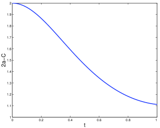
Figure 2: This coefficient measures the importance of the nondiagonal terms in the density matrix. Alternatively, it is the width of the Wigner function. Is shows the rapid decoherence of the unstable particle coupled to a zero temperature environment. Parameters are $\gamma_{0}=0.01$, $\Omega=1$, and $\Lambda=100$.

The main conclusion of this Section is the following. In order to study a sudden quench quantum phase transition, at early times we can use the upside down potential ray ; guthpi ; raynpb . When the system is isolated, due to the high squeezing of the initial wave packet, $x$ and $p$ become classically correlated order . The density matrix is not diagonal. The “correlation time” depends on the shape of the potential. However, when the particle is coupled to an environment, a true quantum to classical transition takes place. The Wigner function becomes peaked around a classical trajectory and the density matrix diagonalizes. The decoherence time at $T=0$ depends on the diffusion coefficients $D$ and $f$ and plays an important role in the early stages of a quantum phase transition, inducing classicality of the order parameter. Quantum aspect could be relevant if non-linearities are taken into account nuno . Decoherence allows a classical description even in the nonlinear regime.

V Acknowledgments

This work was supported by UBA, CONICET, Fundación Antorchas and ANPCyT, Argentina. We would like to thank D. Mazzitelli, D. Monteoliva and J.P. Paz for useful conversations.

References

- (1) See for example, Decoherence and the appearance of a classical world in quantum theory, D. Giulini et al, Springer Verlag (1996).
- (2) W.G. Unruh and W.H. Zurek, Phys. Rev. D40, 1071 (1989).
- (3) W.H. Zurek, “Prefered Sets of States, Predictability, Classicality, and Environment-Induced Decoherence”; in The Physical Origin of Time Asymmetry, ed. by J.J. Halliwell, J. Perez Mercader, and W.H. Zurek (Cambridge University Press, Cambridge, UK, 1994).
- (4) K.E. Nagaev and M. Buttiker, Europhys. Lett., 58(4), 475 (2002).
- (5) G.W. Ford and R.F. O’Connell, J. Optics B5, S349 (2003).
- (6) Y. Imry, arXiv: cond-mat/0202044.
- (7) S. Sinha, Phys. Lett. A228, 1 (1997).
- (8) P. Mohanty, E.M.Q. Jariwala, and R.A. Webb, Phys. Rev. Lett. 78, 3366 (1997).
- (9) B.L. Altshuler, A.G. Aronov, and D.E. Khmelnitsky, J. Phys. C: Solid State Phys., 15, 7367 (1982).
- (10) J.P. Paz and W.H. Zurek, Environmet-induced decoherence and the transition from quantum to classical, lectures at the 72nd Les Houches Summer School on ”Coherent Matter Waves”; (1999). arXiv: quant-ph/0010011.
- (11) J.P. Paz, S. Habib, and W.H. Zurek, Phys. Rev. D47, 488 (1993).
- (12) J.P. Paz and L. Dávila Romero, Phys. Rev. A55, 4070 (1997).
- (13) A. Guth and S.Y. Pi, Phys. Rev D32, 1899 (1985).
- (14) F.C. Lombardo, F.D. Mazzitelli, and D. Monteoliva, Phys. Rev. D62, 045016 (2000).
- (15) B.L. Hu, J.P. Paz, and Y. Zhang, Phys. Rev. D45, 2843 (1993).
- (16) A.D. Viñales, Tesis de Licenciatura en Física, (M.Sc. in Physics); University of Buenos Aires, unpublished (2002).
- (17) F.C. Lombardo, F.D. Mazzitelli, and R.J. Rivers, Phys. Lett. B523, 317 (2001).
- (18) F.C. Lombardo, F.D. Mazzitelli, and R.J. Rivers, Nucl. Phys. B672, 462 (2003).
- (19) N.D. Antunes, F.C. Lombardo, and D. Monteoliva, Phys. Rev. E64, 066118 (2001).