Coherence Control of Adiabatic Decoherence in a Three-level Atom with Lambda Configuration

Abstract

In this paper, we study the suppression of adiabatic decoherence in a three-level atom with $\Lambda$ configuration using bang-bang control technique. We have given the decoupling bang-bang operation group, and programmed a sequence of periodic radio frequency twinborn pulses to realize the control process. Moreover, we have studied the process with non-ideal situation and established the condition for efficient suppression of adiabatic decoherence.

I INTRODUCTION

In recent years, there have been increased interests in the study of three-level quantum systems, for example in quantum cryptography r1 , quantum communication r2 , logic qubit encodingr3 , entanglement measures r4 ; r5 ; r6 , quantum control r7 ; r8 ; r9 , quantum computation r10 . In these areas, people are always confronted with the obstacle of decoherence, by which the superposition of the quantum states is destructed during the system evolution. Preserving coherence is essential in quantum information processing, hence solutions must be sought to dynamically suppress the decoherence effects.

Up to date, several classes of schemes of decoherence control have been proposed, for example, error-correcting, error-avoiding codes and dynamic decoupling technique. The error-correcting codes r11 ; r12 ; r13 ; r14 ; r15 ; r16 ; r17 use conditional feedback control to compensate the loss of information due to decoherence or dissipation. Error-avoiding codes r18 ; r19 ; r20 decouples the interaction between the quantum system and the environment exploiting the symmetry properties of the system and the interaction.

Dynamical decoupling methods have been developed to control decoherencer21 ; r22 ; r23 ; r24 ; r25 ; r26 for decades. Haeberlen and Waugh pioneered the work of coherent averaging effectsr27 using tailored pulse sequence. It has been developed into a solid decoupling and refocusing technique in nuclear magnetic resonance (NMR) r23 ; r29 . Motivated by these ideas, a ”bang-bang” control theory r21 ; r22 has been proposed to dynamically suppress the decoherence by repetitively imposing a sequence of radio-frequency pulses on a single qubit. This active dynamical control in the bang-bang limit proves a nice tool for engineering the evolution of coupled quantum subsystems. In this paper, we will apply the bang-bang control technique to suppress the decoherence induced by pure dephasing in a three-level atom with $\Lambda$ configuration.

II Problem formulation

The system we consider is a three-level atom with $\Lambda$ configuration under two resonant laser fields fields with frequencies

$$\omega_{20}=\frac{E_{2}-E_{0}}{\hbar},\,\,\omega_{21}=\frac{E_{2}-E_{1}}{\hbar},$$

respectively, as shown in Fig.1. Let $|0\rangle$, $|1\rangle$ and $|2\rangle$ be the eigenstates of the unperturbed part of the hamiltonian ${\cal H}_{0}$ of atom, and the corresponding eigenvalues are $E_{0}$, $E_{1}$ and $E_{2}$ respectively and we assume $E_{0}<E_{1}<E_{2}$. The two lower levels $|0\rangle$ and $|1\rangle$ are coupled to a single upper level $|2\rangle$ in the $\Lambda$ type.

Figure 1: Three-level atom in the $\Lambda$ configuration shooting with two fields of frequencies $\omega_{20}$ and $\omega_{21}$

The total hamiltonian of the three-level atom can be expressed as ${\cal H}={\cal H}_{0}+{\cal H}_{R.F.}$, where

$${\cal H}_{0}=E_{0}|0\rangle\langle 0|+E_{1}|1\rangle\langle 1|+E_{2}|2\rangle\langle 2|$$ (1)

is the free hamiltonian and

$${\cal H}_{R.F.}=-(g_{20}|2\rangle\langle 0|+g_{02}^{*}|0\rangle\langle 2|){\cal E}_{1}\cos\omega_{20}t-(g_{21}|2\rangle\langle 1|+g_{12}^{*}|1\rangle\langle 2|){\cal E}_{2}\cos\omega_{21}t$$ (2)

represents the interaction of the atom with the radiation fields.

Here we assume that the electric fields are linearly polarized along the $x$-axis; $g_{ij}=g_{ji}^{*}=e\langle i|x|j\rangle$ $(i,j=0,1,2)$ is the matrix element of the electric moment; ${\cal E}_{i}$ represents the amplitude of the electric field.

Before carrying out the calculation, we define some notation

$$\sigma_{z}^{(2,1)}\equiv|2\rangle\langle 2|-|1\rangle\langle 1|,$$ (3)

$$\sigma_{x}^{(2,1)}\equiv|2\rangle\langle 1|+|1\rangle\langle 2|,$$ (4)

$$\sigma_{y}^{(2,1)}\equiv i(|2\rangle\langle 1|-|1\rangle\langle 2|),$$ (5)

$$\sigma_{+}^{(2,1)}\equiv|2\rangle\langle 1|,$$ (6)

$$\sigma_{-}^{(2,1)}\equiv|1\rangle\langle 2|.$$ (7)

The operators $\sigma_{x}^{(2,0)}$, $\sigma_{x}^{(1,0)}$, $\sigma_{y}^{(1,0)}$, $\sigma_{y}^{(2,0)}$, $\sigma_{z}^{(2,0)}$ and $\sigma_{z}^{(1,0)}$ can be defined similarly. With these notations, the hamiltonian can be rewritten as

$${\cal H}_{0}=\frac{\hbar\omega_{10}}{3}\sigma_{z}^{(1,0)}+\frac{\hbar\omega_{20}}{3}\sigma_{z}^{(2,0)}+\frac{\hbar\omega_{21}}{3}\sigma_{z}^{(2,1)}+\frac{E_{0}+E_{1}+E_{2}}{3}.$$ (8)

where

$$\omega_{10}=\frac{E_{1}-E_{0}}{\hbar},\omega_{20}=\frac{E_{2}-E_{0}}{\hbar},\omega_{21}=\frac{E_{2}-E_{1}}{\hbar}.$$

Usually, the constant energy $(E_{0}+E_{1}+E_{2})/3$ is ignored.

For simplicity, we assume $g_{12}(=g_{21}^{*})$ and $g_{10}(=g_{01}^{*})$ are real numbers. Then

$${\cal H}_{R.F.} =-g_{21}\cos\omega_{21}t\sigma_{x}^{(2,1)}-g_{20}\cos\omega_{20}t\sigma_{x}^{(2,0)}$$ (10)

$$\equiv{\it u}_{1}(t)\sigma_{x}^{(2,0)}+{\it u}_{2}(t)\sigma_{x}^{(2,1)}.$$

Including the decoherence of the system due to the coupling to a thermal reservoir, the total hamiltonian is

$${\cal H}={\cal H}_{0}\otimes{\cal I}_{E}+{\cal I}_{S}\otimes{\cal H}_{E}+{\cal H}_{\it SE}+{\cal H}_{R.F.},$$ (11)

where ${\cal H}_{0}$ and ${\cal H}_{R.F.}$ are the hamiltonians described in (8) and (10). ${\cal H}_{E}$ and ${\cal H}_{\it I}$ describe the internal hamiltonian of the environment and its coupling hamiltonian to the three-level system.

The heat bath is modelled as a large number of uncoupled bosonic modes, namely a reservoir of simple harmonic oscillators with ground state energy shifted to zeror23 ; r24 ; r25 ; r26 ; r27 ,

$${\cal H}_{E}=\sum\limits_{k}\hbar\omega_{k}a_{k}^{\dagger}a_{k}.$$ (12)

The interaction hamiltonian is expressed as

$${\cal H}_{\it SE}=\hbar\sum\limits_{k1}\sigma_{z}^{(2,0)}(g_{k1}a_{k1}^{\dagger}+g_{k1}^{*}a_{k1})+\hbar\sum\limits_{k2}\sigma_{z}^{(2,1)}(g_{k2}a_{k2}^{\dagger}+g_{k2}^{*}a_{k2}).$$ (13)

where $g_{k1}$ and $g_{k2}$ are the coupling constants corresponding to the virtual exchanges of excitations with the bath $|2\rangle\leftrightarrow|0\rangle$ and $|2\rangle\leftrightarrow|1\rangle$ transitions respectively.

Usually, we assume that the initial state of the total system is disentangled, i.e.

$$\rho_{total}(0)=\rho_{S}(0)\otimes\rho_{E}(0),$$

and the thermal reservoir $\rho_{E}(0)$ is in thermal equilibrium state that can be factorized into the tensor product of the density operators of each mode

$$\rho_{E}=\prod\limits_{k}\theta_{k}$$ (14)

where

$$Z_{k} = [1-\exp(-\frac{\hbar\omega_{k}}{k_{B}T})]$$

$$\theta_{k} = Z_{k}^{-1}\exp(-\frac{\hbar\omega_{k}a_{k}^{\dagger}a_{k}}{k_{B}T})$$

where $k_{B}$ is the Boltzmann constant and $T$ is the temperature of the bath.

III Dynamical Suppression of Decoherence in a three-level atom in the ideal limits

Firstly, we sketch the main ideas of the dynamical decoupling theoryr29 ; r30 ; r31 . A bang-bang operation is a unitary operation that can be performed instantaneously, namely corresponding hamiltonian can be turned on for negligible amounts of time $\tau$ with arbitrarily large strength. Let $G_{B.B.}$ be the group consists of the implementable bang-bang operations. The decoupling group ${\cal G}$ is defined as a finite group of bang-bang decoupling operations, ${\cal G}=\{g_{k}\}\subseteq G_{B.B.}$, where $k$ belongs to some finite index set $K$. Then a decoupling-controller on ${\cal H}$ is defined as the interactions of the system, including a sequence of bang-bang operations and free evolution.

Assume the cyclic time is $T_{c}$. Similar to the average hamiltonian theoryr26 ; r28 , we consider a given evolution between the interval $(t-t_{0})=NT_{c}\equiv N|{\cal G}|\Delta t$ in the presence of decoupling-controller characterized by a sequence of bang-bang operators $\{g_{k}\},(k=0,...,|{\cal G}|-1)$. In a single cycle time $T_{c}$, $U(T_{c})=\prod\limits_{k=0}^{|{\cal G}|-1}g_{k}^{+}U_{0}(\Delta t)g_{k}\equiv e^{-i{\cal H}_{eff}T_{c}}$. In the ideal limit of $T_{c}\rightarrow 0$ and $N\rightarrow\infty$, the effective hamiltonian ${\cal H}$ approaches

$${\cal H}_{eff}=\frac{1}{|{\cal G}|}\sum\limits_{k=0}^{|{\cal G}|-1}g_{k}^{+}{\cal H}g_{k}=\Pi_{{\cal G}}({\cal H}),$$

where $\Pi_{{\cal G}}({\cal H})$ can be looked upon as a projector for operator ${\cal H}$ with the following propertiesr30 :

1. projecting ${\cal H}$ into the centralizer $Z({\cal G})$: $Z({\cal G})=\{X\in End({\cal H}_{S}^{space})|[X,g_{k}]=0,\forall k\}$;

2. linearity:$\prod_{{\cal G}}({\cal H})=\Pi_{{\cal G}}({\cal H}_{S}\otimes I_{E})+\Pi_{{\cal G}}(I_{S}\otimes{\cal H}_{E})+\Pi_{{\cal G}}({\cal H}_{SE})$.

From the first property, the effective hamiltonian has a direct symmetry characterization $[{\cal H}_{eff},{\cal G}]=0$, and this implies the composite system with decoherence is symmetrized by the group ${\cal G}$, i.e. all the components of the dynamics generated by ${\cal H}$, which are not invariant under the group ${\cal G}$, can be filtered out from the system’s dynamics. When $\Pi_{{\cal G}}({\cal H}_{SE})=0$, one can find from the second property that the decoherence dynamics induced by the interaction between the system and its environment has been averaged out. Therefore, we can make use of this novel property to design bang-bang control schemes with the dynamical decoupling group ${\cal G}$ to suppress the decoherence.

Applying the above ideas to the three-level atom with $\Lambda$ configuration with a dephasing interactions characterized by Eq. (13), we have found by trials and errors one decoupling group ${\cal G}=\{I,h_{1},h_{2}\}$, where

$$I=\left(\begin{array}[]{ccc}1&0&0\\ 0&1&0\\ 0&0&1\end{array}\right),h_{1}=\left(\begin{array}[]{ccc}0&0&i\\ -1&0&0\\ 0&i&0\end{array}\right),h_{2}=\left(\begin{array}[]{ccc}0&-1&0\\ 0&0&-i\\ -i&0&0\end{array}\right),$$ (15)

and they satisfy the following symmetrization equations

$$\frac{1}{3}(\sigma_{z}^{(2,0)}+h_{1}^{\dagger}\sigma_{z}^{(2,0)}h_{1}+h_{2}^{\dagger}\sigma_{z}^{(2,0)}h_{2})=0,$$ (16)

and

$$\frac{1}{3}(\sigma_{z}^{(2,1)}+h_{1}^{\dagger}\sigma_{z}^{(2,1)}h_{1}+h_{2}^{\dagger}\sigma_{z}^{(2,1)}h_{2})=0.$$ (17)

It is very interesting to note that these bang-bang operations can be decomposed into

$$h_{1}=\left(\begin{array}[]{ccc}1&0&0\\ 0&0&i\\ 0&i&0\end{array}\right)\left(\begin{array}[]{ccc}0&0&i\\ 0&1&0\\ i&0&0\end{array}\right)=\exp(i\frac{\pi}{2}\sigma_{x}^{(2,1)})\exp(i\frac{\pi}{2}\sigma_{x}^{(2,0)}),$$ (18)

and

$$h_{2}=\left(\begin{array}[]{ccc}0&0&-i\\ 0&1&0\\ -i&0&0\end{array}\right)\left(\begin{array}[]{ccc}1&0&0\\ 0&0&-i\\ 0&-i&0\end{array}\right)=\exp(-i\frac{\pi}{2}\sigma_{x}^{(2,0)})\exp(-i\frac{\pi}{2}\sigma_{x}^{(2,1)}).$$ (19)

From these expressions, it is immediate to design a physical realization for these operations using two R.F. pulses as given in Eq. (10) with appropriate frequencies that interact with state transitions $|2\rangle\leftrightarrow|0\rangle$ and $|2\rangle\leftrightarrow|1\rangle$ respectively. For example, $h_{1}$ can be realized by two twinborn pulses, i.e. applying a $\pi$-pulse with frequency $\omega_{20}$ at first and followed by another $\pi$-pulse with frequency $\omega_{21}$. $h_{2}$ is realized similarly.

With the above results, we can design a procedure to effectively suppress the adiabatic decoherence with a sequence of periodic twinborn pulses. In an elementary cycle, the twinborn-pulse sequence is $\{h_{1},h_{1}^{\dagger},h_{2},h_{2}^{\dagger}\}$, as shown in Fig. 2.

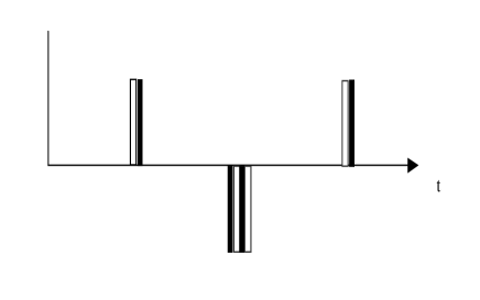
Figure 2: A sequence of twinborn pulse operating in a cycle on the three-level atom. The solid line represents the pulses with frequency of $\omega_{21}$, and the hollow line represents the pulses with frequency of $\omega_{20}$; $\pi$ pulses are on the upside and $-\pi$ pulses are on the downside

In the first half of a cycle, system evolves under ${\cal H}={\cal H}_{0}+{\cal H}_{E}+{\cal H}_{I}$ during $t_{0}\leq t\leq t_{P}^{(1)}\equiv t_{0}+\Delta t$; at time $t_{P}^{(1)}$ twinborn-pulse $h_{1}$ is applied; after $2\tau_{P}$ units of time, the pulse is switched off; then the system is governed by ${\cal H}$ during $t_{P}^{(1)}+2\tau_{P}\leq t\leq t_{P}^{(2)}\equiv t_{0}+2\Delta t$, where $\tau_{P}$ is the pulse width of each sub-pulse of the twinborn-pulse. In the second half of the cycle, the twinborn-pulses $h_{1}^{\dagger}$ and $h_{2}$ is applied and at time $t_{P}^{(2)}$ and $t_{P}^{(2)}+2\tau_{P}$ respectively; after another $2\tau_{P}$ units of time, the pulse is switched off and the system evolves freely under ${\cal H}$ during $t_{P}^{(2)}+4\tau_{P}\leq t\leq t_{P}^{(3)}\equiv t_{0}+3\Delta t$. At time $t_{P}^{(3)}$ the twinborn-pulses of $h_{2}^{\dagger}$ begin. These complete a cycle. By repeating such sequence of elementary cycles, one can suppress the adiabatic decoherence completely in the ideal limits of $T_{c}\rightarrow 0$ and $N\rightarrow\infty$.

IV Dynamical Suppression of Decoherence in a three-level atom with nonideal conditions

In last section, it is shown that the decoherence can be completely removed in the ideal limits of $T_{c}\rightarrow 0$ and $N\rightarrow\infty$. However, the ideal limits that $T_{c}\rightarrow 0$ and $N\rightarrow\infty$ cannot be exactly fulfilled in reality. In this section, we will give a quantitative analysis of effect of finite width and finite-amplitude pulses on the decoherence suppression.

The problem can be reformulated in the interaction picture. Let ${\cal H}^{0}={\cal H}_{0}+{\cal H}_{E}$, then under the standard state transformation $\exp(-i{\cal H}^{0}t)$, the interaction ${\cal{H}}_{SE}$ reads

$$\tilde{{\cal H}}_{\it SE}=\hbar\sum\limits_{k1}\sigma_{z}^{(2,0)}(g_{k1}a_{k1}^{\dagger}e^{i\omega_{k1}t}+g_{k1}^{*}a_{k1}e^{-i\omega_{k1}t})$$

$$+\hbar\sum\limits_{k2}\sigma_{z}^{(2,1)}(g_{k2}a_{k2}^{\dagger}e^{i\omega_{k2}t}+g_{k2}^{*}a_{k2}e^{-i\omega_{k2}t}),$$ (20)

and the free unitary evolution of the composite system is

$$\tilde{U}(t_{0},t)=\exp^{\frac{\sigma_{z}^{(2,0)}}{2}\sum\limits_{k1}[a_{k1}^{\dagger}e^{i\omega_{k1}t_{0}}\xi_{k1}(t-t_{0})-h.c.]}$$

$$\times\exp^{\frac{\sigma_{z}^{(2,1)}}{2}\sum\limits_{k2}[a_{k2}^{\dagger}e^{i\omega_{k2}t_{0}}\xi_{k2}(t-t_{0})-h.c.]}$$ (21)

where

$$\xi_{k1}(\Delta t) = \frac{2g_{k1}}{\omega{k1}}(1-e^{i\omega_{k1}\Delta t})$$

$$\xi_{k2}(\Delta t) = \frac{2g_{k2}}{\omega{k2}}(1-e^{i\omega_{k2}\Delta t}).$$

During an elementary cycle between time $t_{0}$ and $t_{1}=t_{0}+3\Delta t+2\tau_{p}$, the state propagator can be written as

$$\tilde{U}_{P}(t_{0},t_{1})=\tilde{U}_{P4}\tilde{U}(t_{P}^{(2)}+4\tau_{P},t_{P}^{(3)})\tilde{U}_{P3}\tilde{U}_{P2}\tilde{U}(t_{P}^{(1)}+2\tau_{P},t_{P}^{(2)})\tilde{U}_{P1}\tilde{U}(t_{0}^{(1)},t_{P}^{(1)}),$$ (22)

where

$$\tilde{U}_{P1} =e^{i{\cal H}^{0}(t_{P}^{(1)}+\tau_{P})}e^{i\frac{\pi}{2}\sigma_{x}^{(2,1)}}e^{-i{\cal H}^{0}(t_{P}^{(1)}+\tau_{P})}$$ (23)

$$\times e^{i{\cal H}^{0}(t_{P}^{(1)}}e^{i\frac{\pi}{2}\sigma_{x}^{(2,0)}}e^{-i{\cal H}^{0}(t_{P}^{(1)})}$$

$$\approx e^{i{\cal H}^{0}(t_{P}^{(1)})}h_{1}e^{-i{\cal H}^{0}(t_{P}^{(1)})}$$

and likewise,

$$\tilde{U}_{P2}\approx e^{i{\cal H}^{0}(t_{P}^{(2)})}h_{1}^{\dagger}e^{-i{\cal H}^{0}(t_{P}^{(2)})}$$

$$\tilde{U}_{P3}\approx e^{i{\cal H}^{0}(t_{P}^{(2)})}h_{2}e^{-i{\cal H}^{0}(t_{P}^{(2)})}$$

$$\tilde{U}_{P4}\approx e^{i{\cal H}^{0}(t_{P}^{(3)})}h_{2}^{\dagger}e^{-i{\cal H}^{0}(t_{P}^{(3)})}.$$ (24)

Substituting Eqs.(18,19) into Eq.(24), we obtain

$$\tilde{U}(t_{0},t) = e^{\frac{\sigma_{z}^{(2,0)}}{2}\sum\limits_{k1}[a_{k1}^{\dagger}e^{i\omega_{k1}t_{0}}\xi_{k1}(\Delta t)-h.c.]}$$ (25)

$$\times e^{h_{1}^{\dagger}\frac{\sigma_{z}^{(2,0)}}{2}h_{1}\sum\limits_{k1}[a_{k1}^{\dagger}e^{i\omega_{k1}t_{0}}e^{i\omega_{k1}\Delta t}\xi_{k1}(\Delta t)-h.c.]}$$

$$\times e^{h_{2}^{\dagger}\frac{\sigma_{z}^{(2,0)}}{2}h_{2}\sum\limits_{k1}[a_{k1}^{\dagger}e^{i\omega_{k1}t_{0}}e^{i\omega_{k1}2\Delta t}\xi_{k1}(\Delta t)-h.c.]}$$

$$\times e^{\frac{\sigma_{z}^{(2,1)}}{2}\sum\limits_{k2}[a_{k2}^{\dagger}e^{i\omega_{k2}t_{0}}\xi_{k2}(t-t_{0})-h.c.]}$$

$$\times e^{h_{1}^{\dagger}\frac{\sigma_{z}^{(2,1)}}{2}h_{1}\sum\limits_{k2}[a_{k2}^{\dagger}e^{i\omega_{k2}t_{0}}e^{i\omega_{k2}\Delta t}\xi_{k2}(\Delta t)-h.c.]}$$

$$\times e^{h_{2}^{\dagger}\frac{\sigma_{z}^{(2,1)}}{2}h_{2}\sum\limits_{k2}[a_{k2}^{\dagger}e^{i\omega_{k2}t_{0}}e^{i\omega_{k2}2\Delta t}\xi_{k1}(\Delta t)-h.c.]}$$

$$\times e^{i{\cal H}_{0}(t_{1}-t_{0})}.$$

Imposing the above pulse sequences repeatedly, we then get the general expression of the evolution under $N$ bang-bang control cycles

$$\tilde{U}_{P}^{(N)}(t_{0},..,t_{N})=\tilde{U}_{P}(t_{N-1},t_{N})...\tilde{U}_{P}(t_{1},t_{2})\tilde{U}_{P}(t_{0},t_{1}),$$

where $t_{n}=t_{0}+3n\Delta t(n=1,..,N)$ is the ending time of the $n$-th bang-bang control cycle.

With Eq.(25) and more careful calculations, we arrive at

$$\tilde{U}_{P}^{(N)} = e^{\frac{\sigma_{z}^{(2,0)}}{2}\sum\limits_{k1}[a_{k1}^{\dagger}e^{i\omega_{k1}t_{0}}f(n,N,\omega_{k1},\Delta t)\xi_{k1}(\Delta t)-h.c.]}$$ (26)

$$\times e^{-\frac{\sigma_{z}^{(2,1)}}{2}\sum\limits_{k1}[a_{k1}^{\dagger}e^{i\omega_{k1}t_{0}}f(n,N,\omega_{k1},\Delta t)\xi_{k1}(\Delta t)e^{i\omega_{k1}\Delta t}-h.c.]}$$

$$\times e^{-\frac{\sigma_{z}^{(1,0)}}{2}\sum\limits_{k1}[a_{k1}^{\dagger}e^{i\omega_{k1}t_{0}}f(n,N,\omega_{k1},\Delta t)\xi_{k1}(\Delta t)e^{i\omega_{k1}2\Delta t}-h.c.]}$$

$$\times e^{\frac{\sigma_{z}^{(2,1)}}{2}\sum\limits_{k2}[a_{k2}^{\dagger}e^{i\omega_{k2}t_{0}}f(n,N,\omega_{k2},\Delta t)\xi_{k2}(\Delta t)-h.c.]}$$

$$\times e^{\frac{\sigma_{z}^{(1,0)}}{2}\sum\limits_{k2}[a_{k2}^{\dagger}e^{i\omega_{k2}t_{0}}f(n,N,\omega_{k2},\Delta t)\xi_{k2}(\Delta t)e^{i\omega_{k2}\Delta t}-h.c.]}$$

$$\times e^{-\frac{\sigma_{z}^{(2,0)}}{2}\sum\limits_{k2}[a_{k2}^{\dagger}e^{i\omega_{k2}t_{0}}f(n,N,\omega_{k2},\Delta t)\xi_{k2}(\Delta t)e^{i\omega_{k2}2\Delta t}-h.c.]}$$

$$\times e^{iN{\cal H}_{0}3\Delta t},$$

where $f(n,N,\omega,\Delta t)=\sum\limits_{n=1}^{N}e^{3i(n-1)\omega\Delta t}.$

Now we can give a quantitative estimation of the decoherence rate according to the time dependence of non-diagonal matrix elements of the reduced density matrix of the three-level atom. For example, the coherence between the level $|0\rangle$ and $|2\rangle$ is represented by

$$\tilde{\rho}_{02}^{S}(t) = {\rm Tr}_{E}\{\langle 0|\tilde{U}_{P}^{(N)}\tilde{\rho}^{S}(0)\otimes\tilde{\rho}_{E}(0)\tilde{U}_{P}^{(N)\dagger}|2\rangle\}$$

$$= \tilde{\rho}_{02}^{S}(0)Tr_{E}\left[\tilde{\rho}_{E}(0)\exp\{\sum\limits_{k1}a_{k1}^{\dagger}e^{i\omega_{k1}t_{0}}\eta_{k1}(\Delta t)+\sum\limits_{k2}a_{k2}^{\dagger}e^{i\omega_{k2}t_{0}}\eta_{k2}(\Delta t)-h.c\}\right]\exp\{-i3N\omega_{20}\Delta t\}$$

$$= \tilde{\rho}_{02}^{S}(0)\exp\{-i3N\omega_{20}\Delta t-\Gamma(k1,\Delta t)-\Gamma(k2,\Delta t)\},$$

where

$$\Gamma(k1,\Delta t)\equiv\sum\limits_{k1}\frac{|\eta_{k1}(\Delta t)|^{2}}{2}\coth(\frac{\omega_{k1}}{2T}),$$

$$\Gamma(k2,\Delta t)\equiv\sum\limits_{k2}\frac{|\eta_{k2}(\Delta t)|^{2}}{2}\coth(\frac{\omega_{k2}}{2T}),$$

and

$$\eta_{k1}(\Delta t)=-\frac{1}{2}f(n,N,\omega_{k1},\Delta t)\xi_{k1}(\Delta t)(2-e^{i\omega_{k1}\Delta t}-e^{i\omega_{k1}2\Delta t}),$$

and

$$\eta_{k2}(\Delta t)=-\frac{1}{2}f(n,N,\omega_{k2},\Delta t)\xi_{k2}(\Delta t)(1+e^{i\omega_{k1}\Delta t}-2e^{i\omega_{k1}2\Delta t}).$$

On the other hand, the density matrix without the bang-bang control is

$$\tilde{\rho}_{02}^{SW}(t)=\tilde{\rho}_{02}^{S}(0)e^{e^{-i3N\omega_{20}\Delta t}-\Gamma^{{}^{\prime}}(k1,\Delta t)-\Gamma^{{}^{\prime}}(k2,\Delta t)},$$ (27)

where

$$\Gamma^{{}^{\prime}}(k1,\Delta t) \equiv \sum\limits_{k1}\frac{|\xi_{k1}(N,\Delta t)|^{2}}{2}\coth(\frac{\omega_{k1}}{2T})$$

$$\xi_{k1}(N,\Delta t) = f(n,N,\omega_{k1},\Delta t)\xi_{k1}(\Delta t),$$

and

$$\Gamma^{{}^{\prime}}(k2,\Delta t) \equiv \sum\limits_{k2}\frac{|\xi_{k2}(N,\Delta t)|^{2}}{2}\coth(\frac{\omega_{k2}}{2T})$$

$$\xi_{k2}(N,\Delta t) = f(n,N,\omega_{k2},\Delta t)\xi_{k2}(\Delta t).$$

Physically, there exists a finite cutoff frequency of the environment $\omega_{c}$r26 ; r31 . For a single mode of frequency $\omega_{k}$, the time needed to produce appreciable dephasing is $\tau_{k}=\omega_{k}^{-1}$, so $\tau_{c}\sim\omega_{c}^{-1}$ sets the shortest time scale (or memory time) of the environment. When $\omega_{k}\Delta t\in[0,\arccos(\frac{3}{4})]$, we get that $\Gamma(k,\Delta t)\leq\Gamma^{{}^{\prime}}(k,\Delta t)$, which means in the quiet regime $\Delta t\leq\tau_{c}\arccos(\frac{3}{4})$ the pulses will effectively suppress the decoherence.

In addition, $\Gamma(k,\Delta t)$ depends monotonously on the cycle time $\Delta t$. In the ideal limit of $\Delta t\rightarrow 0(N\rightarrow\infty)$, the decoherence is completely suppressed as a result of symmetrization. To show this, we numerically simulate one of the dephasing factors, $\Gamma(k2,\Delta t)$. In the continuum limit of the bath mode, we can see

$$\Gamma_{2}\equiv\Gamma(k2,\Delta t)=\int\limits_{0}^{+\infty}d\omega I(\omega)\times\frac{|\eta_{k2}(\Delta t)|^{2}}{2}\coth\frac{\omega}{2T},$$ (28)

where $I(\omega)=\frac{\alpha}{4}\omega^{n}e^{-\omega/\omega_{c}}$, and $\alpha$ measures the strength of the system-bath interaction and the index $n$ classifies different environmental behaviors. For instance, the Ohmic environment corresponds to $n=1$. From Fig. 3, we can see that the bigger the $N$(or smaller the $\Delta t$), the more effective the bang-bang operation in suppressing the dephasing decoherence.

Figure 3: Decoherence factor $\exp(-\Gamma_{2})$ in the presence of periodical pulses at low-temperature, $\frac{\omega_{c}}{T}=100$. Here $\alpha=0.25$. For a fixed time, each point corresponds to a number of cycles, $N=1,..,N_{max}$. The maximum number of bang-bang control cycles is $N_{max}=30$ for $\omega_{c}t=10$.

V Summary

In this paper, we have studied the suppression of adiabatic decoherence of the three-level atom with $\Lambda$ configuration using bang-bang control technique. The decoupling bang-bang operation group is found, and the sequence of periodic R.F. twinborn pulses is developed for the realization of the control strategy. Moreover, we give a quantitative estimation of the decoherence suppression in non-ideal limits. We also give the condition of effectively suppressing this decoherence.

This work is supported by the National Fundamental Research Program Grant No. 001CB309308, China National Natural Science Foundation Grant No. 10325521, 60433050, 60074015,the Hang-Tian Science Fund, and the SRFDP program of Education Ministry of China.

References

(1) T. Durt, N. J. Cerf, N. Gisin and M. Zukowski, Phys. Rev. A. 67,
012311 (2003).
(2) C. Brukner, M. Zukowski, A. Zeilinger, Phys. Rev. Lett. 89, 197901
(2002).
(3) A. Grudka and A. Wojcik, Phy. Lett.A 314, 350 (2003).
(5) J. L. Cereceda,
xxx.lanl.gov/quant-ph/0305043.
(6) H. Barnum, E. Knill, G. Ortiz, R. Somma and L. Viola, Phys. Rev. Lett. 92, 107902
(2004).
(7) U. Boscain, G. Charlot, J-P. Gauthier, Optimal control of the Schr odinger equation
with two or three levels, in Nonlinear and adaptive control
(Sheffield, 2001), 33 C43, Lecture Notes in Control and Inform.
Sci., 281, Springer, Berlin, 2003.
(8) D. D’Alessandro,
xxx.lanl.gov/quant-ph/0307129
(9) Shlomo E. Sklarz and David J.Tannor,
arXiv:quant-ph/0402143 v1 19 Feb 2004.
(11) A. R. Calderbank and P. W. Shor, Phys. Rev. A.
54, 1098 (1996); P. W. Shor, Phys. Rev. A. 52 R2493
(1995).
(12) R. Laflamme, C. Miquel, J. P. Paz and W. H. Zurek,
Phys. Rev. Lett. 77, 198
(1996).
(13) W. H. Zurek and R. Laflamme, Phys. Rev. Lett. 77, 4683
(1996).
(14) D. Gottesman, Phys. Rev. A. 54, 1862
(1996).
(15) J. I. Cirac et al., Science 273, 1207
(1996).
(16) L. M. Duan and G. C. Guo, Phys. Rev.
Lett. 79, 1953(1997).
(17) S. Lloyd and Slotine Jean-JacquesE, Phys. Rev. Lett. 80,
4088 (1998).
(18) P. Zanardi and M. Rasetti, Phy. Rev. Lett. 79,
3306 (1997).
(19) L. M. Duan and G. C. Guo Phys. Rev. A. 57, 2399
(1997).
(20) I. L. Chuang and Y. Yamamoto, Phys. Rev. A. 52,
3489 (1995).
(21) L. Viola and S. Lloyd, Phys. Rev. A. 58, 2733
(1998).
(22) C. D’ Helon, V. Protopopescu, and R. Perez,
J. Phys.A 36, 7129 (2003).
(23) D. Loss and D. P. DiVincenzo, arXiv: cond-mat/0304118 .
(24) R. P. Feynman and A. R. Hibbs, Quantum Mechanics 8 and Path
Integrals (McGraw-Hill, NY, 1965).
(25) A. O. Caldeira and A. J. Leggett, Phys. Rev. Lett.46,
211 (1981).
(26) A. J. Leggett, S. Chakravarty, A. T. Dorsey, M. P. A.
Fisher and W. Zwerger,Rev. Mod. Phys.59, 1 (1987)
(27) S. Swain, J. Phys.A 5, 1587 (1972.
(28) P. Zanardi, Phy. Lett.A 258, 77 (1999).
(29) L. Viola, Phy. Rev.A 66, 012307 (2002).
(30) L. Viola, S. Lloyd and E. Knill,Phy. Rev. Lett.83,
4888 (1999).
(31) L. Viola, E. Knill and S. Lloyd, Phy. Rev. Lett.82,
2417 (1999).
(32) U. Haeberlen and J.S. Waugh, Phys. Rev.175, 453, 1968.
(33) U. Haeberlen, High Resolution NMR in Solids: Selective
Averaging (Academic Press, New York), 1976; R. R. Ernst, G.
Bodenhausen, and A. Wokaun, Principles of Nuclear Magnetic
Resonance in One and Two Dimensions, Oxford University Press,
Oxford, 1994.