Kochen-Specker Algorithms for Qunits

Abstract

Algorithms for finding arbitrary sets of Kochen-Specker (KS) qunits ($n$-level systems) as well as all the remaining vectors in a space of an arbitrary dimension are presented. The algorithms are based on linear MMP diagrams which generate orthogonalities of KS qunits, on an algebraic definition of states on the diagrams, and on nonlinear equations corresponding to MMP diagrams whose solutions are either KS qunits or the remaining vectors of a chosen space depending on whether the diagrams allow 0-1 states or not. The complexity of the algorithms is polynomial. New results obtained with the help of the algorithms are presented.

1 Introduction

In quantum measurements, particular directions of quantisation axes of the measured observable obey the following KS conditions: (1) no two of mutually orthogonal directions can both be assigned 1; (2) they cannot all be assigned 0. Zimba and Penrose (1993) To these directions we ascribe vectors that we call KS vectors. To stress that the axes and therefore KS vectors themselves cannot be given a 0-1 valuation, i.e. represented by classical bits, we also call them KS qunits (quantum n-ary digits). We are not aiming at giving yet another proof of the KS theorem but at determining the class of all KS vectors from an arbitrary ${\cal H}^{n}$ as well as the class of all the remaining vectors from ${\cal H}^{n}$. In other words, our aim is to obtain all physically realisable vectors in ${\cal H}^{n}$ corresponding to orientations of projectors.

In order to achieve this aim, we first recognise that a description of a discrete observable measurement (e.g., spin) in ${\cal H}^{n}$ can be rendered as a 0-1 measurement of the corresponding projectors along orthogonal vectors in ${\mathbb{R}}^{n}$ to which the projectors project. Hence, we deal with orthogonal triples in ${\mathbb{R}}^{3}$, quadruples in ${\mathbb{R}}^{4}$, etc., which correspond to possible experimental designs. To find KS vectors means finding all such $n$-tuples in ${\mathbb{R}}^{n}$ that correspond to experiments which have no classical counterparts.

2 MMP diagrams and their generation

We represent the $n$-tuples in ${\mathbb{R}}^{n}$ by means of points of a diagram. The points are called vertices. Groups of orthogonal vectors are represented by connected vertices and are called edges. Vertices and edges form linear MMP diagrams McKay et al. (2000); Pavičić (2002) which are defined as follows:

1. Every vertex belongs to at least one edge;

2. Every edge contains at least 3 vertices;

3. Every edge which intersects with another edge at least twice contains at least 4 vertices.

The procedure for generation MMP diagrams follows from isomorphism-free generation of linear diagrams established in McKay et al. (2000); Pavičić (2002); McKay (1998). Here we present the main idea behind such a generation and will present the details elsewhere. Pavičić et al. (2005)

The algorithm for obtaining MMP diagrams is based on the parent-child generation tree as the one shown in Fig. 1 for the particular number of vertices and loops we allow (it will be shown below that for 3 vertices per edge no diagram containing loops of size less then 5 can generate a set of vectors). At every further level we add an edge until we reach a desired number of vertices and edges. In doing so the main problem is to avoid generation of diagrams isomorphic to an already generated diagram. This is resolved by using the procedure given below. The procedure guarantees that at each parent level generation of isomorphic children is suppressed. E.g., each of the two diagrams at the third level could give the third diagram at the fourth level. However, the generation procedure prevents the second generation.

procedure scan $(D$ : diagram; $\beta$ : integer$)$

if $D$ has exactly $\beta$ edges then

output $D$

else

for each equivalence class of extensions $D+e$ do

if $e\in m(D+e)$ then scan($D+e$,$\beta$)

end procedure

It is the function $m(\cdot)$ which we define in McKay et al. (2000) that enables us to define a unique isomorphism class as the parent class of the isomorphism class of $D$. This way of generation of diagrams enables a very efficient parallelisation of computing on clusters. The complexity of generation grows exponentially and if we had not integrated its algorithm with the related algorithms for solving the corresponding non-linear equations we would not have been able to realistically implement the generation of MMP diagrams. Because, e.g., there are 6 3-vertices-per-edge and smallest loops of size 5 diagrams with 19 vertices and 13 edges and already 7447274324 diagrams with 29 vertices and 20 edges, etc.

We denote vertices of MMP diagrams by 1,2,..,A,B,..a,b,.. By the above algorithm we generate MMP diagrams with chosen numbers of vertices and edges and a chosen minimal loop size.

3 0-1 states on MMP diagrams

To find diagrams that do not allow 0-1 states we use an algorithm which carries exhaustive search on MMP diagrams with backtracking. The idea of the algorithm follows from our elaboration on states in the Hilbert space. Megill and Pavičić (2000) Essentially, the algorithm ascribes non-dispersive (0-1) states so as to assign 1 to exactly one vertex within an edge while the other vertices within the edge are assigned 0. The algorithm scans the vertices in some order, trying 0 then 1, skipping vertices constrained by an earlier assignment. When no assignment becomes possible, the algorithm backtracks until all possible assignments are exhausted or a valid assignment is found. Again, the algorithm by itself would be exponential, but the constraints build up quickly so that the exponential behaviour of the algorithm is reduced to a polynomial one.

In Fig. 2 (a) the smallest diagram with 4 vertices per edge and with the smallest loop of size 2 (two edges share two vertices) which does not admit 0-1 states is shown. It has 6 vertices and 3 edges, so it is denoted as 6-3. We can write it down as follows: 1234,2356,1456. Fig. 2 (b) shows one of the two smallest diagrams with 3 vertices per edge and smallest loops of size 5 that do not admit 0-1 states: 19-13: 123,345,567,789,9AB,BCD,DE1,2GA,4HC,6IG,6JD,8FE,FGH.

4 Kochen-Specker Qunits

To obtain KS qunits we merge the algorithms for generation of linear MMP diagrams corresponding to edges of orthogonal vectors in ${\mathbb{R}}^{n}$ (Sec. 2), algorithms for filtering out those vectors on which 0-1 states cannot be defined (Sec. 3), and algorithms for solving nonlinear equations describing the orthogonalities of the vectors by means of interval analysis so as to eventually generate KS vectors in a polynomially complex way.

Following the idea put forward in Pavičić (2002) we proceed so as to require that the vertices correspond to vectors from ${\mathbb{R}}^{n}$, that the number of vertices within edges corresponds to the dimension of ${\mathbb{R}}^{n}$, and that edges correspond to $n(n-1)/2$ equations resulting from inner products of vectors being equal to zero which means orthogonality. An example for the edge BCD in ${\mathbb{R}}^{3}$ is shown by Eq. (1).

Combinations of edges for a chosen number of vertices and chosen number of orthogonalities between them correspond to a system of such nonlinear equations.

$${\mathbf{a}}_{B}\cdot{\mathbf{a}}_{C}=a_{B1}a_{C1}+a_{B2}a_{C2}+a_{B3}a_{C3}=0,$$

$${\mathbf{a}}_{B}\cdot{\mathbf{a}}_{D}=a_{B1}a_{D1}+a_{B2}a_{D2}+a_{B3}a_{D3}=0,$$

$${\mathbf{a}}_{C}\cdot{\mathbf{a}}_{D}=a_{C1}a_{D1}+a_{C2}a_{D2}+a_{C3}a_{D3}=0.$$ (1)

However, we cannot first generate all possible MMP diagrams and only afterwards try to filter them by solving equations because their number grows exponentially and the required time for such a generation on the fastest CPU would exceed the age of the universe for any application of interest. Instead, we restrict generation of MMP diagrams so that as soon as a preliminary pass determines that an initial set of $m$ $n$-tuples has no solution, no further systems containing this set will be generated and the whole sub-tree in the generation tree is discarded. E.g., for 18 vertices and 12 quadruple edges without such a restriction one should generate $>2.9\cdot 10^{16}$ systems—what would require more than 30 million years on a 2 GHz CPU—while the filter reduces the generation to 100220 systems (obtainable within $<30$ mins on a 2 GHz CPU). Thereafter we get 26800 systems without 0-1 states in $<5$ secs. We also developed a checking program that finds solutions from assumed sets, say $\{-1,0,1\}$, even much faster ($<$ 1 sec on a 2 GHz CPU).

For the remaining systems two solvers have been developed. One is based on a specific implementation of Ritt characteristic set calculation and the other on the interval analysis, in particular the library ALIAS. We will elaborate on these solvers and present further details of the algorithms elsewhere. Pavičić et al. (2005)

5 Some Results

Using our general algorithms presented above, we wrote programs Pavičić et al. (2005) which provided us with a number of special results that show the power of the algorithms.

(i) A general feature we found to hold for all MMP diagrams without 0-1 states we tested is that the number of vertices $a$ and the number of edges $b$ satisfy the following inequality: $nb\geq 2a$, where $n$ is the number of vertices per edge. In ${\mathbb{R}}^{n}$ this means that we cannot arrive at systems with more unknown (components of vectors) then equations (orthogonality conditions). The biggest systems we tested contain 30 vertices. There is only one system known to us—containing 192 vertices—for which the inequality is violated. Pavičić et al. (2005)

(ii) Several self-explaining results are presented in Fig. 3. As we can see, two of them have miraculously been previously found by some ingenious humans (think of billions of positions the vectors can take).

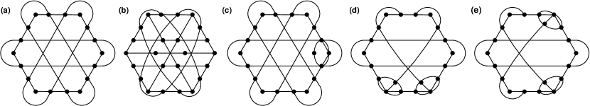
Fig. 3: Smallest 4-dim KS vectors with:  (1)  loops of size 3: (a) 18-9 (isomorphic to Cabello et al. Cabello et al. (1996)); (b) 24(22)-13 not containing (a), with values $\not\in\{-1,0,1\}$;  (2)  loops of size 2: (2.1) containing (a): (c) 19(18)-10; (2.2) not containing (a): (d) 20-11-a; (e) 20-11-b (isomorphic to Kernaghan Kernaghan (1994)). Solutions are given in Pavičić et al. (2005).

(iii) Between 4-dim systems, with smallest loops of size 3, (a) and (b) of Fig. 3, there are 62 systems with loops of size 3, all containing the system (a), but 37 of whom do not have solutions from $\{-1,0,1\}$. System (b) is the first system not containing (a); it does not have a solution from $\{-1,0,1\}$. The solution is given in  Pavičić et al. (2005).

(iv) All 4-dim systems with up to 22 vectors and 12 edges with the smallest loops of size 2 which do have solutions from $\{-1,0,1\}$ contain at least one of the systems (d) and (e) and in many cases also (a) of Fig. 3. The two smallest 4-dim systems with the smallest loops of size 2 that contain neither of the latter three systems are 22-13 systems (a) and (b) of Fig. 4: 1234,4567,789A,ABCD,DEFG,GHI1,2ILA,345J,4JEC,678K,7KMG,9ABL,FGHM and 1234,4567,789A,ABCD,DEFG,GHI1,12IJ,345K,678L,GML7,1J9B,4KEC,FGHM.

(v)    (c) and (d) of Fig. 4 are two presentations of the same 24-24 KS system: 1234,4567,789A,ABCD,DEFG, GHI1, 12IJ, 345K, 678L, 7LOG, 68FH, 1J9B, AMI2, 4KCE, DN35, CDEN, IJK5, 38KL, 6BML, 9EMN,CHNO,2JOF,9ABM,OFGH that make it easier to recognise that the system contains all the previous systems: (a), (c), (d), and (e) of Fig. 3 and (a) and (b) of Fig. 4. The vectors determined by the solution of the system are nothing but Peres’ vectors Peres (1991), although he has most probably never tried to identify all 24 tetrads for his 24 vectors (our programs verify all these options in a fraction of a second). We also developed a program for drawing MMP diagrams. Megill and Pavičić (2000)

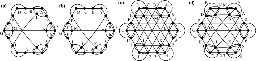
Fig. 4: (a) and (b): Smallest KS systems systems (22-13) containing neither (a) nor (c) nor (d) nor (e) of Fig. 3. Solutions are given in Pavičić et al. (2005); (c) and (d) (isomorphic to each other) are a 24-24 KS system containing (a), (c), (d), and (e) of Fig. 3 and all Peres’ vectors Peres (1991).

(v) 4-dim systems with more than 41 vectors cannot have solutions from $\{-1,0,1\}$ and there are no such solutions to systems with minimal loops of size 5 up to 41 vectors, what brings the Hasse (Greechie) diagram approach to the KS problem into question. Up to 41 vertices with loops of size 5 there are only two diagrams that have no 0-1 states.

(vi) It can easily be shown that a 3-dim system of equations representing diagrams containing loops of size 3 and 4 cannot have a real solution. Pavičić et al. (2005)

(vii) We scanned all systems with up to 30 vectors and 20 orthogonal triads and there are no KS vectors among them. This does not mean that Conway-Kochen’s system is the smallest KS system, though. Pavičić et al. (2005) It turns out that we cannot drop vectors that belong to only one edge from orthogonal triads because there are cases where a solution to a full system allows 0-1 valuation while one to a system with dropped vectors does not or where the full system cannot have a solution. So, Conway-Kochen’s system is actually not a 31 but a 51 vector system. Pavičić et al. (2005) See also Larsson (2002).

(viii) The class of all remaining (non-KS) vectors from ${\cal H}^{n}$ we get so as to first filter out all the MMP diagrams that do have 0-1 states. Then the real solutions to the equations corresponding to these diagrams yield the desired vectors.

(ix) Presented algorithms can easily be generalised beyond the KS theorem. One can use MMP diagrams to generate Hilbert lattices, partial Boolean algebras, and general quantum algebras which could eventually serve as an algebra for quantum computers. Megill and Pavičić (2000) One can also treat any condition imposed upon inner products in ${\mathbb{R}}^{n}$ to find solutions not by directly solving all nonlinear equations but by first filtering the corresponding diagrams and solving only those equations that pass the filters.

References

- Zimba and Penrose (1993) Zimba, J., and Penrose, R., Stud. Hist. Phil. Sci., 24, 697–720 (1993).
- McKay et al. (2000) McKay, B. D., Megill, N. D., and Pavičić, M., Int. J. Theor. Phys., 39, 2381–2406 (2000), arXiv.org/quant-ph/0009039.
- Pavičić (2002) Pavičić, M., “Quantum Computers, Discrete Space, and Entanglement,” in SCI 2002/ISAS 2002 Proceedings, The 6th World Multiconference on Systemics, Cybernetics, and Informatics, edited by N. Callaos, Y. He, and J. A. Perez-Peraza, SCI, Orlando, Florida, 2002, vol. XVII, SCI in Physics, Astronomy and Chemistry, pp. 65–70, arXiv.org/quant-ph/0207003.
- McKay (1998) McKay, B. D., J. Algorithms, 26, 306–324 (1998).
- Pavičić et al. (2005) Pavičić, M., Merlet, J.-P., McKay, B. D., and Megill, N. D., J. Phys. A, 38 (2005), arXiv.org/quant-ph/9907072.
- Megill and Pavičić (2000) Megill, N. D., and Pavičić, M., Int. J. Theor. Phys., 39, 2337–2379 (2000), arXiv.org/quant-ph/0009038.
- Cabello et al. (1996) Cabello, A., Estebaranz, J. M., and García-Alcaine, G., Phys. Lett. A, 212, 183–187 (1996), arXiv.org/quant-ph/9706009.
- Kernaghan (1994) Kernaghan, M., J. Phys. A, 27, L829–L830 (1994).
- Peres (1991) Peres, A., J. Phys. A, 24, L175–L178 (1991).
- Larsson (2002) Larsson, J.-Å., Europhys. Lett., 58, 799–805 (2002), arXiv.org/quant-ph/0006134.