Multi-particle entanglement manipulation under positive partial transpose preserving operations

Abstract

We consider the transformation of multi-partite states in the single copy setting under positive-partial-transpose-preserving operations (PPT-operations) and obtain both qualitative and quantitative results. Firstly, for some pure state transformations that are impossible under local operations and classical communication (LOCC), we demonstrate that they become possible with a surprisingly large success probability under PPT-operations. Furthermore, we clarify the convertibility of arbitrary multipartite pure states under PPT-operations, and show that a drastic simplification in the classification of pure state entanglement occurs when the set of operations is switched from LOCC to PPT-operations. Indeed, the infinitely many types of LOCC-incomparable entanglement are reduced to only one type under the action of PPT-operations. This is a clear manifestation of the increased power afforded by the use of PPT-bound entanglement. In addition, we further enlarge the set of operations to clarify the effect of another type of bound entanglement, multipartite unlockable bound entanglement, and show that a further simplification occurs. As compared to pure states a more complicated situation emerges in the mixed state settings. While single copy distillation becomes possible under PPT-operations for some mixed states it remains impossible for other mixed states.

I Introduction

Constraints and resources are intimately related in physics. If we impose a constraint on a physical setting then certain tasks become impossible. A resource must be made available to overcome the restrictions imposed by the constraints. By definition such a resource cannot be created employing only the constrained set of operations but it may be manipulated and transformed under these operations. That the amount of resource does not increase under any operation satisfying the constraint emerges then as a fundamental law, for example in entanglement theory Plenio98a ; Eisert03a .

One example of particular importance is the restriction to local quantum operations and classical communication (LOCC). The resource that is implied by this constraint are non-separable states and in particular pure entangled states such as singlet states, neither of which can be created by LOCC alone. This setting gives rise to a theory of entanglement as a resource under LOCC operations.

Any such theory of entanglement as a resource will generally aim to provide mathematical structures to allow answers to three questions, namely (1) the characterization of entanglement, (2) the manipulation of entanglement and (3) the quantification of the entanglement resource Plenio98a ; Eisert03a under the given constraint. Of particular interest is the question of how many inequivalent types of entanglement exist within such a theory. In the limit of infinitely many identically prepared copies of bipartite pure states, entanglement can be inter-converted reversibly Bennett96b and it is reasonable to say that there is only one type of pure bipartite entanglement. Even for pure states, the situation changes dramatically when we consider the single copy setting. It has been shown that the Schmidt rank of bipartite pure states cannot be increased by LOCC Lo97a ; Nielsen99a ; Vidal99a ; Jonathan99a ; Jonathan99b . At the single copy level, the convertibility of bipartite entanglement is then characterized by the Schmidt-rank Dur00b . For finite dimensional systems a state can be converted to another one with finite probability exactly if the Schmidt-number of the target state is not larger than that of the initial state. In a tripartite setting the situation is more complicated. Here it is well-known for example that a GHZ state cannot be transformed to a $W$ state and vice versa Dur00b . These states are then said to be incomparable. It can be shown that there are two incomparable types of tripartite entanglement in three qubits systems. The situation is even more complicated in multipartite settings composed by many parties Verstraete02a ; Miyake03a ; Verstraete03a ; Briand03a ; Miyake04a or infinite dimensional bipartite systems Owari04a ; Eisert SP02 , where there are many (possibly infinitely many) incomparable types of entanglement.

A different setting is presented by the concept of partial time reversal or partial transposition Peres96a . For two qubits, states that remain positive under partial transposition (denoted as PPT-states) are exactly the separable states Horodecki96a but for higher dimensions this is generally not the case as there are PPT-states that are inseparable Horodecki98a . This motivates the definition of the set of positive-partial-transpose-preserving operations (PPT-operations), defined as operations that map any PPT-state into another PPT-state Rains01a . In this case, the resource are states that are not PPT (denoted as NPT-states). In the single copy setting for pure states, it has been shown that both under PPT-operations Audenaert03a and with LOCC supported by PPT-bound entanglement Ishizaka04b the Schmidt-number can be increased so that state transformations become possible that are strictly impossible under LOCC. Furthermore, there are mixed state transformations that are reversible in the asymptotic setting Audenaert03a . This suggests that a theory of entanglement under PPT-operations might have a much simpler structure than that under the LOCC constraint.

In this paper, we focus attention on the entanglement manipulation under PPT operations in the non-asymptotic, single copy setting to explore what simplification occur. We consider PPT state transformation in multipartite settings and obtain both qualitative and quantitative results. In Sec. II, the general settings and notations of PPT preserving operations are introduced. In Secs. III and IV, we first demonstrate that the transformations of pure states that are impossible under LOCC become possible with a surprisingly large success probability when employing trace preserving PPT-operations. In Secs. V, a rather tractable scheme of trace non-preserving PPT-operations is introduced and discussed. We will then completely clarify the convertibility of all multipartite pure states under PPT-operations in Sec. VI. In Sec. VII we enlarge the set of operations beyond that of PPT-operations to consider the effect of multipartite unlockable bound entangled states. In Sec. VIII, we will consider the transformation of a single copy of mixed states into pure entangled states, i.e. the single copy distillation under PPT-operations. A summary and conclusion is given in Sec. IX.

II Basic notation

To begin with, let us denote ${\cal H}(V)$ (${\cal H}(V^{\prime})$) the space of Hermitian operators on the Hilbert space $V$ ($V^{\prime}$). A superoperator $\Psi$ from $V$ to $V^{\prime}$ is a linear transformation from ${\cal H}(V)$ to ${\cal H}(V^{\prime})$. There is a natural isomorphism Rains01a which associates with superoperators $\Psi:{\cal H}(V)\rightarrow{\cal H}(V^{\prime})$ a Hermitian operator $\Omega(\Psi)\in{\cal H}(V)\otimes{\cal H}(V^{\prime})$ such that for all $A\in{\cal H}(V)$ and $B\in{\cal H}(V^{\prime})$ we have

$$\hbox{tr}\{\Psi(A)B\}=\hbox{tr}\{\Omega(\Psi)A\otimes B\}.$$ (1)

Maps that are trace non-increasing then satisfy

$$\hbox{tr}_{V^{\prime}}\{\Omega({\Psi})\}\leq\openone_{V}$$ (2)

with equality if $\Psi$ is trace preserving. A superoperator $\Psi$ is called positive if for any $A\geq 0$ we have $\Psi(A)\geq 0$ and it is called completely positive if $\openone_{W}\otimes\Psi\geq 0$ for any space $W$. Following Rains01a complete positivity (CP) of $\Psi$ can be verified by checking

$$\Omega(\Psi)^{\Gamma_{V}}\geq 0$$ (3)

where $\Gamma_{V}$ denotes the partial transposition with respect to $V$.

An additional concept comes into play when we consider multipartite systems. A CP-map on bipartite systems $\Psi:{\cal H}(V_{A})\otimes{\cal H}(V_{B})\rightarrow{\cal H}(V^{\prime}_{A})\otimes{\cal H}(V^{\prime}_{B})$ is called positive partial transpose preserving (PPT) Rains01a , if we have $\Gamma_{A}\circ\Psi\circ\Gamma_{A}\!\geq\!0$ ($\Gamma_{B}\circ\Psi\circ\Gamma_{B}\!\geq\!0$) for the partial transposition map $\Gamma_{A}$ ($\Gamma_{B}$) with respect to party $A$ ($B$). On the level of the state $\Omega(\Psi)$, this condition reads

$$(\Omega(\Psi)^{\Gamma_{V}})^{\Gamma_{V_{A}}\otimes\Gamma_{V^{\prime}_{A}}}\geq 0\hbox{~{}~{}or~{}~{}}(\Omega(\Psi)^{\Gamma_{V}})^{\Gamma_{V_{B}}\otimes\Gamma_{V^{\prime}_{B}}}\geq 0$$

where $\Gamma_{V_{A}}$ ($\Gamma_{V^{\prime}_{A}}$) denotes partial transposition applied to space $V_{A}$ $(V^{\prime}_{A})$. In the bipartite case, there are two equivalent choices for the partial transposition. In the tripartite setting however, there are three different possible partial transpositions that are generally not equivalent. A CP map $\Psi:{\cal H}(V_{A})\otimes{\cal H}(V_{B})\otimes{\cal H}(V_{C})\rightarrow{\cal H}(V^{\prime}_{A})\otimes{\cal H}(V^{\prime}_{B})\otimes{\cal H}(V^{\prime}_{C})$ will be called PPT in the following if

$$(\Omega(\Psi)^{\Gamma_{V}})^{\Gamma_{V_{i}}\otimes\Gamma_{V^{\prime}_{i}}}\geq 0$$ (4)

for all $i\!=\!A$, $B$ and $C$.

Let us now consider the transformation of a state $\rho\in{\cal H}(V)$ into a state $\sigma\in{\cal H}(V^{\prime})$ with the probability of $p(\rho\!\rightarrow\!\sigma)$. For this probabilistic transformation, we construct the trace preserving CP-PPT map with two outcomes, one that gives $\sigma$ and one that gives some other state. The two parts are given by CP-PPT maps $\Psi$ and $\psi$, respectively. The associated Hermitian operators are denoted by $\Omega$ and $\omega$. The map $\Psi$ then satisfies $\Psi(\rho)\!=\!p(\rho\!\rightarrow\!\sigma)\sigma$ or

$$\hbox{tr}\{\Psi(\rho)(\openone-\sigma)\}=\hbox{tr}\{\Omega(\Psi)\rho\otimes(\openone-\sigma)\}=0$$ (5)

when $\sigma$ is a pure state. The success probability is then given by

$$p(\rho\rightarrow\sigma)=\hbox{tr}\{\Psi(\rho)\} = \hbox{tr}\{\Omega(\Psi)\rho\otimes\openone\}$$

$$= \hbox{tr}\{\Omega(\Psi)\rho\otimes\sigma\}.$$

The PPT-map $\psi$, on the other hand, does not suffer any constraint other than the condition of trace-preservation for $\Psi+\psi$. On the level of states, the trace-preserving condition is

$$\hbox{tr}_{V^{\prime}}\{\Omega+\omega\}=\openone_{V},$$ (6)

where, as we will do in the remainder of this paper, we have dropped the $\Psi$ ($\psi$) in $\Omega(\Psi)$ ($\omega(\psi)$) for brevity. It should be noted that a rather simple structure can be assumed for $\omega$ without loss of generality. Let us consider a map $\chi$ which maps arbitrary states in ${\cal H}(V)$ into a maximally mixed state of $\openone_{V^{\prime}}/\hbox{dim}\{{\cal H}(V^{\prime})\}\!\in\!{\cal H}(V^{\prime})$. This map is a trace-preserving CP-PPT map since the corresponding state is $\openone_{V}\otimes\openone_{V^{\prime}}/\hbox{dim}\{{\cal H}(V)\otimes{\cal H}(V^{\prime})\}$. Therefore, a composed map of $\chi\circ\psi$ is a CP-PPT map if $\psi$ is a CP-PPT map. Furthermore, if $\Psi\!+\!\psi$ is trace preserving, $\Psi\!+\!\chi\circ\psi$ is also trace preserving, and hence the replacement of $\psi$ by $\chi\circ\psi$ does not alter $p(\rho\!\rightarrow\!\sigma)$. One may then assume $\psi\!=\chi\circ\psi$ since the output of $\psi$ is arbitrary. On the level of the state, this assumption is

$$\omega=\omega_{V}\otimes\frac{\openone_{V^{\prime}}}{\hbox{dim}\{{\cal H}(V^{\prime})\}}.$$ (7)

In the subsequent Secs. III and IV, we maximize $p(\rho\!\rightarrow\!\sigma)$ for some important classes of pure states in both bipartite and tripartite settings. In particular, we demonstrate that transformations of pure states that are impossible under LOCC can be achieved under PPT operations with a surprisingly large success probability.

III Conversion of maximally entangled states

For two d-dimensional systems we denote the maximally entangled state by $P^{+}_{d}\!\equiv\!|\phi^{+}_{d}\rangle\langle\phi^{+}_{d}|$ where

$$|\phi^{+}_{d}\rangle=\frac{1}{\sqrt{d}}\sum_{i=0}^{d-1}|ii\rangle.$$

In the single copy setting, it is known that LOCC cannot increase the Schmidt rank of a pure state Lo97a ; Nielsen99a ; Vidal99a ; Jonathan99a ; Jonathan99b . Therefore, $p(P^{+}_{d}\!\rightarrow\!P^{+}_{d^{\prime}})=0$ for LOCC transformation whenever $d^{\prime}\!>\!d$.

In the following we proceed with the construction of the CP-PPT maps $\Psi$ and $\psi$ that maximize the success probability for this transformation. For $d^{\prime}\!>\!d$ this amounts to the maximization of

$$p(P^{+}_{d}\rightarrow P^{+}_{d^{\prime}})=\hbox{tr}\{\Omega P^{+}_{d}\otimes P^{+}_{d^{\prime}}\}$$ (8)

under the constraints

$$\hbox{tr}\{\Omega P^{+}_{d}\otimes(\openone-P^{+}_{d^{\prime}})\} = 0,\;\;\hbox{tr}_{V^{\prime}}\{\Omega+\omega\}=\openone,$$

$$(\Omega^{\Gamma_{V_{A}}\otimes\Gamma^{\prime}_{V_{A}}})^{\Gamma_{V}} \geq 0,\hskip 41.25641pt\Omega^{\Gamma_{V}}\geq 0,$$ (9)

$$(\omega^{\Gamma_{V_{A}}\otimes\Gamma^{\prime}_{V_{A}}})^{\Gamma_{V}} \geq 0,\hskip 41.25641pt\omega^{\Gamma_{V}}\geq 0,$$

where $P^{+}_{d}\!\in\!{\cal H}(V)$ and $P^{+}_{d^{\prime}}\!\in\!{\cal H}(V^{\prime})$. Since both $P^{+}_{d}\!\otimes\!P^{+}_{d^{\prime}}$ and $P^{+}_{d}\!\otimes\!(\openone\!-\!P^{+}_{d^{\prime}})$ are invariant under the local unitary transformation of $U_{1}\otimes U^{*}_{1}\otimes U_{2}\otimes U^{*}_{2}$ with $U_{1}$ and $U_{2}$ being arbitrary unitary operators, it suffices to consider $\Omega$ and $\omega$ that are invariant under these local operations, i.e.

$$\Omega = a_{1}P^{+}_{d}\otimes P^{+}_{d^{\prime}}+a_{2}(\openone-P^{+}_{d})\otimes P^{+}_{d^{\prime}}$$

$$+ a_{3}P^{+}_{d}\otimes\frac{\openone-P^{+}_{d^{\prime}}}{{d^{\prime}}^{2}-1}+a_{4}(\openone-P^{+}_{d})\otimes\frac{\openone-P^{+}_{d^{\prime}}}{{d^{\prime}}^{2}-1},$$

$$\omega_{V} = b_{1}P^{+}_{d}+b_{2}(\openone-P^{+}_{d}).$$

The first two constraints in Eq. (9) yield $a_{3}\!=\!0$, $b_{1}\!=\!1-a_{1}$, and $b_{2}\!=\!1-a_{2}-a_{4}$. These equalities can be used to eliminate $b_{1}$ and $b_{2}$ in the remaining constraints. The remaining constraints then result in

$$1\geq a_{1}\geq 0,\;\;a_{2}\geq 0,\;\;a_{4}\geq 0,\;\;1\geq a_{2}+a_{4},$$

$$(d^{\prime}+1)a_{1}+(d^{\prime}+1)(d-1)a_{2}+(d-1)a_{4} \geq 0,$$

$$-(d^{\prime}+1)a_{1}+(d^{\prime}+1)(d+1)a_{2}+(d+1)a_{4} \geq 0,$$

$$-(d^{\prime}-1)a_{1}-(d^{\prime}-1)(d-1)a_{2}+(d-1)a_{4} \geq 0,$$

$$(d^{\prime}-1)a_{1}-(d^{\prime}-1)(d+1)a_{2}+(d+1)a_{4} \geq 0,$$

$$-a_{1}-(d-1)a_{2}-(d-1)a_{4}+d \geq 0,$$

$$a_{1}-(d+1)a_{2}-(d+1)a_{4}+d \geq 0.$$

The constraints in the first row arise from $\omega^{\Gamma_{V}}\!\geq\!0$ and $\Omega^{\Gamma_{V}}\!\geq\!0$. The last two rows are due to $(\omega^{\Gamma_{V_{A}}\otimes\Gamma^{\prime}_{V_{A}}})^{\Gamma_{V}}\!\geq\!0$ and the remaining for inequalities arise from $(\Omega^{\Gamma_{V_{A}}\otimes\Gamma^{\prime}_{V_{A}}})^{\Gamma_{V}}\!\geq\!0$. The maximization of $p(P^{+}_{d}\!\rightarrow\!P^{+}_{d^{\prime}})\!=\!a_{1}$ under these constraints is a linear program and we can identify the optimal solution as $a_{1}\!=\!d(d\!-\!1)/(dd^{\prime}\!+\!d^{\prime}\!-\!2d)$, $a_{2}\!=\!0$, and $a_{4}\!=\!d(d^{\prime}\!-\!1)/(dd^{\prime}\!+\!d^{\prime}\!-\!2d)$. Consequently, for $d^{\prime}>d$ the optimal probability for the transformation of $P^{+}_{d}$ into $P^{+}_{d^{\prime}}$, thereby increasing the Schmidt rank, under PPT-operations is given by

$$p(P^{+}_{d}\rightarrow P^{+}_{d^{\prime}})=\frac{d(d-1)}{dd^{\prime}+d^{\prime}-2d}.$$ (10)

We emphasize that this success probability is nonzero even when $d^{\prime}\!>\!d\!\geq\!2$, while it is strictly zero for the LOCC transformation.

IV Conversion from GHZ to $W$ state

In the tripartite setting, it is well-known that the success probability $p(GHZ\!\rightarrow\!W)=0$ for the LOCC transformation from a single copy of

$$|GHZ\rangle=\frac{|000\rangle+|111\rangle}{\sqrt{2}}$$

to

$$|W\rangle=\frac{|001\rangle+|010\rangle+|100\rangle}{\sqrt{3}}$$

Dur00b . In the following we will demonstrate that this is not the case when we consider PPT-operations. To this end, we maximize

$$p(\rho_{GHZ}\rightarrow\rho_{W})=\hbox{tr}\{\Omega\rho_{GHZ}\otimes\rho_{W}\}$$ (11)

under the constraints for $i=A,B,C$,

$$\hbox{tr}\{\Omega\rho_{GHZ}\otimes(\openone-\rho_{W})\} = 0,\;\;\hbox{tr}_{V^{\prime}}\{\Omega+\omega\}=\openone,$$

$$(\Omega^{\Gamma_{V_{i}}\otimes\Gamma^{\prime}_{V_{i}}})^{\Gamma_{V}} \geq 0,\hskip 41.25641pt\Omega^{\Gamma_{V}}\geq 0,\;\;$$

$$(\omega^{\Gamma_{V_{i}}\otimes\Gamma^{\prime}_{V_{i}}})^{\Gamma_{V}} \geq 0,\hskip 41.25641pt\omega^{\Gamma_{V}}\geq 0,\;\;$$

where $\rho_{GHZ}\!=\!|GHZ\rangle\langle GHZ|\!\in\!{\cal H}(V)$ and $\rho_{W}\!=\!|W\rangle\langle W|\!\in\!{\cal H}(V^{\prime})$.

The solution of the problem is greatly aided by the use of a number of symmetries. Indeed, both the states $\rho_{GHZ}\!\otimes\!(\openone\!-\!\rho_{W})$ and $\rho_{GHZ}\!\otimes\!\rho_{W}$ are invariant under the local operations

$$(a) X\otimes X\otimes X\otimes\,\openone\,\otimes\,\openone\,\otimes\,\openone\,,$$

$$(b) Z\,\otimes Z\,\otimes\,\openone\,\otimes\,\openone\,\otimes\,\openone\,\otimes\,\openone\,,$$

$$(c) \,\openone\,\otimes Z\,\otimes Z\,\otimes\,\openone\,\otimes\,\openone\,\otimes\,\openone\,,$$

$$(d) \,\openone\,\otimes\,\openone\,\otimes\,\openone\,\otimes Z\,\otimes Z\,\otimes Z\,,$$

$$(e) P_{1}\otimes P_{1}\otimes P_{1}\otimes\openone\otimes\openone\,\otimes\openone\,,$$

$$(f) \,\openone\,\otimes\,\openone\,\otimes\,\openone\,\otimes P_{2}\otimes P_{2}\otimes P_{2},$$

where $P_{1}\!=\!|0\rangle\langle 0|\!+\!|1\rangle\langle 1|e^{2\pi i/3}$ and $P_{2}\!=\!e^{\pi i/2}|0\rangle\langle 0|\!+\!|1\rangle\langle 1|e^{\pi i}$. These local symmetries are supplemented by the non-local joint permutation symmetry

$$(g)\;\;{\cal P}(123)\times{\cal P}(456)\hskip 42.67912pt$$

where ${\cal P}$ represents an arbitrary index permutation. The symmetries (a) - (g) allow for a considerable simplification of $\Omega$ and $\omega$. Indeed, the symmetries (b), (c) and (e) ensure that the matrix elements $\Omega_{i_{1}j_{1}k_{1}l_{1}m_{1}n_{1},i_{2}j_{2}k_{2}l_{2}m_{2}n_{2}}$ can only be non-zero if the indices satisfy simultaneously $i_{1}\!=\!i_{2}$, $j_{1}\!=\!j_{2}$ and $k_{1}\!=\!k_{2}$ or $i_{1}\!=\!1\!-\!i_{2}$, $j_{1}\!=\!1\!-\!j_{2}$ and $k_{1}\!=\!1\!-\!k_{2}$. The symmetry (g) yields

$$\Omega_{abcdef,ghijkl}=\Omega_{{\cal P}(abc){\cal P}(def),{\cal P}(ghi){\cal P}(jkl)}$$ (12)

for any index permutation ${\cal P}$. Symmetry (a) yields

$$\Omega_{000l_{1}m_{1}n_{1},000l_{2}m_{2}n_{2}} = \Omega_{111l_{1}m_{1}n_{1},111l_{2}m_{2}n_{2}},$$ (13)

$$\Omega_{001l_{1}m_{1}n_{1},001l_{2}m_{2}n_{2}} = \Omega_{110l_{1}m_{1}n_{1},110l_{2}m_{2}n_{2}},$$ (14)

$$\Omega_{000l_{1}m_{1}n_{1},111l_{2}m_{2}n_{2}} = \Omega_{111l_{1}m_{1}n_{1},000l_{2}m_{2}n_{2}}.$$ (15)

Presenting all nonzero matrix elements of $\Omega_{abcdef,ghijkl}$ for $(abc,ghi)\!=\!(000,000)$, $(abc,ghi)\!=\!(001,001)$ and $(abc,ghi)\!=\!(000,111)$ fixes all other matrix elements by virtue of the symmetries Eqs. (12-15) and the Hermiticity of $\Omega$. To obtain a trial solution we chose

$$\Omega_{000000,000000} \!=\! \Omega_{001000,001000}=-\Omega_{000000,111000}=b_{1},$$

$$\Omega_{000001,000001} \!=\! \Omega_{000001,000010}=\Omega_{000001,000100}=b_{2},$$

$$\Omega_{000011,000011} \!=\! \Omega_{000011,000101}=\Omega_{000011,000110}=b_{4},$$

$$\Omega_{001001,001001} \!=\! -\Omega_{001001,001010}=-\Omega_{001001,001100}=b_{2},$$

$$\Omega_{001010,001010} \!=\! \Omega_{001010,001100}=\Omega_{001100,001100}=b_{2},$$

$$\Omega_{001011,001011} \!=\! \Omega_{001011,001101}=-\Omega_{001011,001110}=-b_{4},$$

$$\Omega_{001101,001101} \!=\! -\Omega_{001101,001110}=\Omega_{001110,001110}=b_{4},$$

$$\Omega_{001111,001111} \!=\! 3\Omega_{000111,000111}=-3\Omega_{000111,111111}=3b_{6},$$

$$\Omega_{000001,111001} \!=\! \Omega_{000001,111010}=\Omega_{000001,111100}=b_{2},$$

$$\Omega_{000010,111010} \!=\! \Omega_{000010,111100}=\Omega_{000100,111100}=b_{2},$$

$$\Omega_{000011,111011} \!=\! \Omega_{000011,111101}=\Omega_{000011,111110}=-b_{4},$$

$$\Omega_{000101,111101} \!=\! \Omega_{000101,111110}=\Omega_{000110,111110}=-b_{4}.$$

Likewise, the non-zero matrix elements of $\omega_{V}$ can be constructed from

$$(\omega_{V})_{000,000} = 1-b_{6}-3b_{4}-3b_{2}-b_{1},$$

$$(\omega_{V})_{001,001} = (\omega_{V})_{000,111},$$

$$(\omega_{V})_{000,111} = b_{6}+3b_{4}-3b_{2}+b_{1},$$

where we chose

$$b_{1} = \frac{1+\sqrt{1-4x^{2}}}{6},\;\;b_{2}=\frac{x}{3},\;\;\;b_{4}=\frac{b_{2}^{2}}{b_{1}},\;\;\;b_{6}=\frac{9b_{4}^{2}}{3x},$$

$$x = \frac{1}{8}(-2+(18-6\sqrt{3})^{1/3}+(18+6\sqrt{3})^{1/3}).$$

A lengthy but elementary calculation (preferably executed employing a program capable of symbolic manipulations) then confirms that this trial solution satisfies all the constraints and yields the success probability

$$\hbox{tr}\{\Omega\rho_{GHZ}\otimes\rho_{W}\}=6b_{2}.$$ (16)

We then consider the dual problem of the primal problem Eq. (11) Boyd04a . Every feasible point of the dual problem provides an upper bound on the solution of the primal problem Eq. (11). The above result of Eq. (16) is then proven to be optimal as shown in Appendix A.

As a consequence, the optimal probability for the transformation of a GHZ to a $W$ state under PPT-operations is given by

$$p(GHZ\rightarrow W)=6b_{2}\approx 0.75436...,$$ (17)

that is more than 75%. This very high success probability is somewhat surprising, since the success probability for the LOCC transformation is strictly zero. Note that this result also implies that a GHZ state can be transformed into a W state employing LOCC supplemented by PPT-bound entanglement.

V Trace non-preserving CP-PPT maps

In the previous two sections we have demonstrated explicitly that the success probability for the transformation between pure states can in some cases be improved significantly by employing PPT-operations instead of LOCC operations. Obtaining the optimal success probabilities is a hard task, however, especially in the multipartite setting. In the following we will consider the slightly more tractable setting of trace non-preserving PPT maps. In this setting we also optimize a CP-PPT map $\Psi$ or equivalently the associated state $\Omega$, but the trace preserving condition of Eq. (6) is replaced by the trace non-increasing condition of

$$\hbox{tr}_{V^{\prime}}\{\Omega\}\leq\openone_{V}.$$ (18)

As a result, the completion $\psi$ of the map $\Psi$ is a CP map but it is not necessarily a PPT map. This will generally allow to find success probabilities for state transformations that are larger than those obtained under trace-preserving PPT operations. It is important to note, however, that any transformation that possesses a non-vanishing success probability under trace non-preserving CP-PPT maps will also have a non-vanishing success probability under trace preserving CP-PPT maps. To see this, let $\Omega(\Psi)$ be the state corresponding to a trace non-preserving CP-PPT map $\Psi$. Since the completion $\psi$ is not necessarily a PPT map, $\omega(\psi)^{\Gamma_{V}}$ is sometimes a NPT-state. However, if we consider the states of $\Omega^{\prime}(\Psi^{\prime})\!=\!\epsilon\Omega(\Psi)$ and $\omega^{\prime}(\psi^{\prime})\!=\!\epsilon\omega(\psi)+(1\!-\!\epsilon)\openone\otimes\openone/{\dim\{{\cal H}(V^{\prime})\}}$, the state $(\omega^{\prime})^{\Gamma_{V}}$ becomes a PPT-state for a nonzero value of $1\!\geq\!\epsilon\!>\!0$. Both $(\Omega^{\prime})^{\Gamma_{V}}$ and $(\omega^{\prime})^{\Gamma_{V}}$ are PPT states satisfying the trace preserving condition of Eq. (6), and $\Psi^{\prime}$ accomplishes the same transformation as $\Psi$ albeit with a smaller success probability. In this way, one can always construct a trace preserving CP-PPT map from the trace non-preserving CP-PPT map giving the same transformation.

The optimal probability in the trace non-preserving scheme for the transformation of maximally entangled states ($d^{\prime}\!>\!d$) can be obtained in the same fashion as section III. Employing the notation of section III we obtain the constraints

$$1\geq a_{1}\geq 0,\;\;\;\;a_{2}\geq 0,\;\;\;\;a_{4}\geq 0,\;\;\;\;1\geq a_{2}+a_{4},$$

$$(d^{\prime}+1)a_{1}+(d^{\prime}+1)(d-1)a_{2}+(d-1)a_{4} \geq 0,$$

$$-(d^{\prime}+1)a_{1}+(d^{\prime}+1)(d+1)a_{2}+(d+1)a_{4} \geq 0,$$

$$-(d^{\prime}-1)a_{1}-(d^{\prime}-1)(d-1)a_{2}+(d-1)a_{4} \geq 0,$$

$$(d^{\prime}-1)a_{1}-(d^{\prime}-1)(d+1)a_{2}+(d+1)a_{4} \geq 0$$

under which the success probability, given by $a_{1}$, has to be maximized. The result is

$$p(P^{+}_{d}\rightarrow P^{+}_{d^{\prime}})=\frac{d-1}{d^{\prime}-1},$$ (19)

whose PPT map $\Psi$ is, on the level of the state $\Omega$,

$$\Omega=\frac{d-1}{d^{\prime}-1}P^{+}_{d}\otimes P^{+}_{d^{\prime}}+\frac{1}{d^{\prime 2}-1}(\openone-P^{+}_{d})\otimes(\openone-P^{+}_{d^{\prime}}).$$ (20)

It is noteworthy that the probability of Eq. (19) can be written as a ratio of the negativity of the initial and target state, i.e.

$$p(P^{+}_{d}\!\rightarrow\!P^{+}_{d^{\prime}})=\frac{N(P^{+}_{d})}{N(P^{+}_{d^{\prime}})}$$

where $N(\sigma)\!=\!(\hbox{tr}|\sigma^{\Gamma}|-1)/2$ Audenaert03a ; Negativity . This somewhat fascinating expression resembles the case of the LOCC transformation of pure states, where the optimal probability agrees with a ratio of a LOCC-monotone such that the partial summation of squared Schmidt coefficients Vidal99a . Although the monotonicity of the negativity in trace non-preserving PPT-operations has not been proved yet (in trace preserving PPT operations with a single outcome the negativity is a monotone Audenaert03a ), the tractable expression of Eq. (19) is likely to be explained as a ratio of some monotone function.

In the tripartite setting, the optimization of the success probability is still a hard task even in this trace non-preserving scheme. The result of the optimization for the transformation of $\hbox{GHZ}\!\rightarrow\!W$ is

$$p(GHZ\rightarrow W)=\frac{4}{5},$$ (21)

and for the transformation of $W\!\rightarrow\!\hbox{GHZ}$ we have

$$p(W\rightarrow GHZ)=\frac{1}{3}.$$ (22)

The proof for these two results are described in appendices B and C. This result implies that the transformation of $W\!\rightarrow\!\hbox{GHZ}$ is also possible by trace preserving PPT-operations, although the optimal probability may be smaller than 1/3. Therefore, PPT-operations can inter-convert even the LOCC-incomparable pure states. In the next section, we will completely clarify the convertibility by PPT-operations for all multipartite pure states in the single copy setting.

VI Convertibility of pure states

In this section we will consider the transformation between single copies of $N$-partite pure states under PPT-operations. By definition, PPT-operations map PPT-states to PPT-states. As a consequence, transformations such as $|\phi^{+}_{AB}\rangle\!\otimes\!|0_{C}\rangle\!\rightarrow\!|GHZ\rangle$ or $|\phi^{+}_{AB}\rangle\!\otimes\!|0_{C}\rangle\!\rightarrow\!|0_{A}\rangle\!\otimes\!|\phi^{+}_{BC}\rangle$ are impossible, since they are not PPT-preserving with respect to party $C$. Therefore, let us first assume for the transformation of $|\psi\rangle\!\rightarrow\!|\phi\rangle$ that both $|\psi\rangle$ and $|\psi\rangle$ are “genuinely” entangled over all $N$ parties. This assumption means that

$$(|\psi\rangle\langle\psi|)^{\Gamma_{i}}\not\geq 0\hbox{~{}~{}~{}and~{}~{}~{}}(|\phi\rangle\langle\phi|)^{\Gamma_{i}}\not\geq 0,$$ (23)

for all possible bipartite partitioning of $i$. For example, $i\!=\!A$, $B$, $C$ in a tripartite setting, and $i\!=\!A$, $B$, $C$, $D$, $AB$, $AC$, $AD$ in a four-partite setting. As discussed in the previous section, it suffices to consider trace non-preserving CP-PPT maps $\Psi$ in order to check the convertibility under trace preserving PPT-operations. Therefore, we will construct an $\Omega$ satisfying the constraints

$$\hbox{tr}\{\Omega|\psi\rangle\langle\psi|\otimes(\openone-|\phi\rangle\langle\phi|)\}=0,$$

$$\;\;\Omega^{\Gamma_{V}}\geq 0,\;\;\;(\Omega^{\Gamma_{V_{i}}\otimes\Gamma^{\prime}_{V_{i}}})^{\Gamma_{V}}\geq 0,$$ (24)

where $|\psi\rangle\!\in\!{\cal H}(V)$, $|\phi\rangle\!\in\!{\cal H}(V^{\prime})$, and $i$ stands for any possible bipartite partitioning as explained below Eq. (23). We have omitted the trace non-increasing condition, because we are not interested in the explicit value of the success probability but only whether it is zero or not. In view of Eq. (20), a suitable trial form is

$$\Omega=x|\psi\rangle\langle\psi|\otimes|\phi\rangle\langle\phi|+(\openone-|\psi\rangle\langle\psi|)\otimes(\openone-|\phi\rangle\langle\phi|),$$ (25)

for which the first two constraints in Eq. (24) are satisfied when $x\!\geq\!0$. Furthermore, due to the assumption of Eq. (23), the last constraint $(\Omega^{\Gamma_{i}\otimes\Gamma^{\prime}_{i}})^{\Gamma_{V}}\!\geq\!0$ is also satisfied for an appropriate value of $x\!=\!x_{0}\!>\!0$ as shown in Ishizaka04b . As a result, for $x\!=\!x_{0}$ we have

$$\hbox{tr}\{\Omega(|\psi\rangle\langle\psi|\otimes|\phi\rangle\langle\phi|)\}=x_{0}>0,$$ (26)

so that for arbitrary pairs of genuine $N$-partite entangled states of $|\psi\rangle$ and $|\phi\rangle$ we can always find an $\Omega$ such that $p(|\psi\rangle\!\rightarrow\!|\phi\rangle)\!>\!0$. As a consequence, all genuine $N$-partite pure entangled states are inter-convertible by PPT-operations. In this way, the classification of $N$-partite entanglement is drastically simplified when we consider PPT-operations.

Let us next investigate the convertibility between a $N$-partite state $|\psi^{(N)}\rangle$ and a $(N\!-\!1)$-partite state $|\phi^{(N-1)}\rangle$. It is obvious that $|\phi^{(N-1)}\rangle\!\rightarrow\!|\psi^{(N)}\rangle$ is impossible because such a transformation is not PPT-preserving. Likewise the transformation of $|\psi^{(N)}\rangle\!\rightarrow\!|\phi^{(N-1)}\rangle$ is impossible if the set of entangled parties in $|\phi^{(N-1)}\rangle$ is not a subset of the set of entangled parties in $|\psi^{(N)}\rangle$ (e.g. $|\psi^{(3)}_{ABC}\rangle\!\rightarrow\!|\phi^{(2)}_{AD}\rangle$ is impossible). Otherwise, the transformation is possible because a $N$-partite GHZ state can be transformed to a $(N\!-\!1)$-partite GHZ state by LOCC, and hence the sequential transformation of $|\psi^{(N)}\rangle\!\rightarrow\!|GHZ^{(N)}\rangle\!\rightarrow\!\!|GHZ^{(N-1)}\rangle\!\rightarrow\!|\phi^{(N-1)}\rangle$ is possible. The classification and convertibility of arbitrary multipartite pure entangled states under PPT-operations are summarized in Fig. 1.

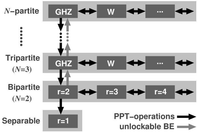
Figure 1: The classification and convertibility of multipartite pure entangled states under PPT-operations. $r$ denotes the Schmidt rank of bipartite entanglement, and the set of entangled parties in $(N\!-\!1)$-partite entanglement is assumed to be a subset of the set of entangled parties in $N$-partite entanglement. There is only one type of $N$-partite entanglement under PPT-operations. Furthermore, the convertibility with the support of unlockable bound entanglement (BE) is also shown (see also Dur99a ).

It is important to note here that the power of PPT-operations, by which $N$-partite pure entangled states becomes inter-convertible as discussed above immediately implies that the same holds for LOCC supported by PPT bound entanglement. This is due to the fact that any PPT-transformation can be accomplished (with smaller but nonzero probability) by LOCC supported by the additional resource of PPT-states Cirac01a (see the note of Note_for_PPT_operations ). Indeed,

$$\Psi(\rho)=\hbox{tr}_{V}\{\Omega(\Psi)^{\Gamma_{V}}(\rho^{\Gamma_{V}}\otimes\openone)\},$$ (27)

and the state of $\Omega(\Psi)^{\Gamma_{V}}\!\geq\!0$, which is a PPT-state if $\Psi$ is a CP-PPT map due to $(\Omega(\Psi)^{\Gamma_{i}\otimes\Gamma^{\prime}_{i}})^{\Gamma_{V}}\!\geq\!0$, is utilized and consumed in the LOCC-implementation of $\Psi(\rho)$ Cirac01a . If a CP-PPT map $\Psi$ can accomplish a transformation that is impossible under LOCC alone, then $\Omega(\Psi)^{\Gamma_{V}}$ must be entangled (otherwise the transformation can also be accomplished by LOCC because LOCC can generate any separable state), and therefore the PPT-state $\Omega(\Psi)^{\Gamma_{V}}$ is a PPT bound entangled state Horodecki98a . Consequently, one can conclude that the transformation such as $\hbox{GHZ}\!\leftrightarrow\!W$ can be accomplished by LOCC with the consumption of PPT bound entangled states. Much attention has been paid to bound entanglement to clarify its properties, and several applications of bound entanglement have been reported Horodecki99c ; Dur99a ; Smolin01a ; Shor03a ; Murao01a ; Dur01a ; Kaszlikowski02a ; Sen02a ; Dur01b ; Horodecki03a ; Dur04a ; Augusiak04a . As shown above, PPT bound entanglement enables the LOCC implementation of large classes of entanglement transformations that are impossible by LOCC alone.

VII Unlockable states and conversion of pure states

As mentioned in the previous section, the transformation

$$|\phi^{+}_{AB}\rangle\otimes|0_{C}\rangle\rightarrow|GHZ_{ABC}\rangle$$ (28)

cannot be achieved even when PPT-operations are employed, and therefore cannot be achieved by LOCC supported by PPT-bound entanglement. However, it has been shown that a GHZ state can be distilled from a tripartite NPT-bound entangled state, if $A$ and $B$ perform a global operation on the state Dur99a . Such NPT-bound entangled states are called unlockable states because bound entanglement is unlocked by the global operation Smolin01a ; Wei04a ; Augusiak04b . The global operation of $A$ and $B$ can be accomplished by LOCC consuming $|\phi^{+}_{AB}\rangle$, and consequently the transformation of Eq. (28) is possible when LOCC is supported by the unlockable bound entanglement Dur99a . Likewise, unlockable states which can be utilized for the LOCC-transformation from a $(N\!-\!1)$-partite GHZ state to a $N$-partite GHZ state have been shown in Dur99a . In this section we consider this type of transformation using a certain general scheme.

To this end, we generalize PPT-operations by relaxing the PPT-preserving condition with respect to $C$, $(\Omega^{\Gamma_{V_{C}}\otimes\Gamma^{\prime}_{V_{C}}})^{\Gamma_{V}}\!\geq\!0$, which is responsible for the impossibility of the transformation of Eq. (28). We will therefore construct a map $\Psi$ whose associated Hermitian operator $\Omega$ satisfies

$$\hbox{tr}\{\Omega P^{+}_{AB}\otimes(\openone-\rho_{GHZ})\}=0,\;\;\Omega^{\Gamma_{V}}\geq 0,$$

$$(\Omega^{\Gamma_{V_{A}}\otimes\Gamma^{\prime}_{V_{A}}})^{\Gamma_{V}}\geq 0,\;\;(\Omega^{\Gamma_{V_{B}}\otimes\Gamma^{\prime}_{V_{B}}})^{\Gamma_{V}}\geq 0,$$ (29)

where $P^{+}_{AB}\!=\!|\phi^{+}_{AB}\rangle\langle\phi^{+}_{AB}|\!\in\!{\cal H}(V)$ and $\rho_{GHZ}\!\in\!{\cal H}(V^{\prime})$. As a trial form for $\Omega$, we adopt again Eq. (25), i.e.

$$\Omega=xP^{+}_{AB}\otimes\rho_{GHZ}+(\openone-P^{+}_{AB})\otimes(\openone-\rho_{GHZ}).$$ (30)

As mentioned in the previous section,

$$(P^{+}_{AB})^{\Gamma_{A}}\not\geq 0\hbox{~{}~{}~{}and~{}~{}~{}}\rho_{GHZ}^{\Gamma_{A}}\not\geq 0$$

ensure the existence of $x_{0}\!>\!0$ such that $(\Omega^{\Gamma_{V_{A}}\otimes\Gamma^{\prime}_{V_{A}}})^{\Gamma_{V}}\!\geq\!0$ for $0\!<\!x\!\leq\!x_{0}$ (indeed, we have $x_{0}\!=\!3$), and likewise with respect to $B$. We can now check easily that all constraints in Eq. (29) are satisfied for $x\!=\!3$, yielding a nonzero success probability $p(|\phi^{+}_{AB}\rangle\!\rightarrow\!|GHZ\rangle)\!>\!0$ since $\hbox{tr}\{\Omega(P^{+}_{AB}\otimes\rho_{GHZ})\}\!>\!0$. Consequently, the transformation of $|\phi^{+}_{AB}\rangle\!\rightarrow\!|GHZ\rangle$ is possible under the set of operations that maps NPT-BE states with respect to party $C$ into itself, as expected. Employing symmetries of $P^{+}_{AB}\otimes\rho_{GHZ}$, the optimized success probability in the trace non-preserving scheme is then obtained as

$$p(|\phi^{+}_{AB}\rangle\!\rightarrow\!|GHZ\rangle)=\frac{3}{5},$$ (31)

and, on the level of states, the map $\Psi$ realizing this success probability is given by

$$\Omega = \frac{3}{5}P^{+}_{AB}\otimes\rho_{GHZ}$$ (32)

$$+ \frac{1}{5}(\openone-P^{+}_{AB})\otimes(\openone-\rho_{GHZ}\!-\!\rho_{001}-\rho_{110}),$$

where $\rho_{001}\!=\!|001\rangle\langle 001|$ and $\rho_{110}\!=\!|110\rangle\langle 110|$. It can be confirmed that the state $\Omega^{\Gamma_{V}}$ is an unlockable state as follows. Due to the constraints of $(\Omega^{\Gamma_{V_{A}}\otimes\Gamma^{\prime}_{V_{A}}})^{\Gamma_{V}}\!\geq\!0$ and $(\Omega^{\Gamma_{V_{B}}\otimes\Gamma^{\prime}_{V_{B}}})^{\Gamma_{V}}\!\geq\!0$, the mixed state of $\Omega^{\Gamma_{V}}$ is undistillable by LOCC, because LOCC is PPT-preserving and no tripartite and bipartite pure entangled state exists that is PPT with respect to both $A$ and $B$. However, a GHZ state can be distilled from $\Omega^{\Gamma_{V}}$ of Eq. (30) or Eq. (32), if $A$ and $B$ perform global operations that distinguish $P^{+}_{AB}$ and $\openone\!-\!P^{+}_{AB}$.

Similarly, the map $\Psi$, whose associated state is

$$\Omega=3\rho_{GHZ}^{(N)}\otimes\rho_{GHZ}^{(N^{\prime})}+(\openone\!-\!\rho_{GHZ}^{(N)})\otimes(\openone\!-\!\rho_{GHZ}^{(N^{\prime})}),$$ (33)

can transform a $N$-partite GHZ state ($\rho_{GHZ}^{(N)}$) to a $N^{\prime}$-partite GHZ state, and furthermore the state $\Omega^{\Gamma_{V}}$ is an unlockable state if $N^{\prime}\!>\!N\!\geq\!2$ Note_for_unlockable_state . As shown in the previous section, all genuine $N$-partite entangled states are inter-converted by PPT maps. The composition of the PPT maps and the map given in Eq. (33) is again a map whose associated state is an unlockable state. This implies that all pure entangled states can be inter-converted independently of the number of parties ($N$) when a single copy of an appropriate unlockable bound entangled state is available as a resource. In this way, the consumption of unlockable bound entanglement allows to overcome the LOCC-constraint between pure states with different sets of entangled parties, while the consumption of PPT bound entanglement overcomes the LOCC-constraint between pure states with the same set of entangled parties (Fig. 1).

VIII Single copy distillation

So far, we have concentrated our attention on the discussion of transformations between pure states. In this section, we will now consider the transformation of a single copy of a mixed state $\rho$ into a maximally entangled state $P^{+}_{d^{\prime}}$, i.e. the single copy distillation from a mixed state employing PPT-operations.

Let us consider the antisymmetric Werner state which is defined as

$$\sigma^{a}_{d}=\frac{2}{d^{2}-d}P^{a}_{d}=\frac{2}{d^{2}-d}\sum_{j>i}|\psi^{-}_{ij}\rangle\langle\psi^{-}_{ij}|,$$ (34)

where $P^{a}_{d}$ is the projector onto the antisymmetric subspace of ${\mathbb{C}}^{d}\otimes{\mathbb{C}}^{d}$, and $|\psi^{-}_{ij}\rangle\!=\!(|ij\rangle\!-\!|ji\rangle)/\sqrt{2}$. For the transformation of $\sigma^{s}_{d}\!\rightarrow\!P^{+}_{d^{\prime}}$, we can construct CP-PPT maps of $\Psi$ and its CP-PPT completion $\psi$ employing the twirling symmetries of the two states. The result of the optimization is, on the level of the state $\Omega$ (the state $\omega$ is given by $\omega_{V}\!=\!\openone\!-\!\hbox{tr}_{V^{\prime}}\Omega$),

$$\Omega=\frac{2}{dd^{\prime}+d^{\prime}-2d}\Big{[}P^{a}_{d}\otimes P^{+}_{d^{\prime}}+(d^{\prime}-1)P^{s}_{d}\otimes\frac{\openone-P^{+}_{d^{\prime}}}{{d^{\prime}}^{2}-1}\Big{]}$$

for $d^{\prime}\!\geq\!d\!\geq\!2$, and

$$\Omega = \frac{2}{d(d^{\prime}-1)}\Big{[}P^{a}_{d}+\frac{(d-d^{\prime})}{(d+1)d^{\prime}}P^{s}_{d}\Big{]}\otimes P^{+}_{d^{\prime}}$$

$$+ \frac{2(d^{\prime}+1)}{(d+1)d^{\prime}}P^{s}_{d}\otimes\frac{\openone-P^{+}_{d^{\prime}}}{{d^{\prime}}^{2}-1}$$

for $2\!\leq\!d^{\prime}\!\leq\!d$ where $P^{s}_{d}$ is the projector onto the symmetric subspace of ${\mathbb{C}}^{d}\otimes{\mathbb{C}}^{d}$. The optimal success probability under trace preserving CP-PPT-operations is then given by

$$p(\sigma^{a}_{d}\rightarrow P^{+}_{d^{\prime}})=\left\{\begin{array}[]{lc}\displaystyle\frac{2}{dd^{\prime}+d^{\prime}-2d}&\hbox{~{}for $d^{\prime}\!>\!d\!\geq\!2$,}\\[8.5359pt] \displaystyle\frac{2}{d(d^{\prime}-1)}&\hbox{~{}for $2\!\leq\!d^{\prime}\!\leq\!d$.}\end{array}\right.$$ (35)

Therefore, the success probability is nonzero for $d^{\prime}\!\geq\!2$.

On the other hand, the success probability for the same transformation under LOCC operations alone is strictly zero whenever $d^{\prime}\!>\!2$. This can be proven as follows: The $|\psi^{-}_{ij}\rangle$ in Eq. (34) are maximally entangled states on ${\mathbb{C}}^{2}\otimes{\mathbb{C}}^{2}$. Therefore, each $|\psi^{-}_{ij}\rangle$ can be prepared from $P^{+}_{2}$ by local unitary transformations only. As $\sigma^{a}_{d}$ is an equal mixture of all possible $|\psi^{-}_{ij}\rangle$, $\sigma^{a}_{d}$ can be prepared from a single copy of $P^{+}_{2}$ by LOCC, and hence the transformation of $P^{+}_{2}\!\rightarrow\!\sigma^{a}_{d}$ has a finite success probability. If we furthermore assume that for $d^{\prime}\!>\!2$ the transformation $\sigma^{a}_{d}\!\rightarrow\!P^{+}_{d^{\prime}}$ has a finite success probability under LOCC, then this implies that $P^{+}_{2}\!\rightarrow\!\sigma^{a}_{d}\!\rightarrow\!P^{+}_{d^{\prime}}$ also has a finite success probability under LOCC. This contradicts that the Schmidt rank cannot be increased by LOCC. Therefore, the result of Eq. (35) implies that the success probability of the single copy distillation is also significantly improved when PPT-operations are considered.

It should be noted that the transformation of $\sigma^{a}_{d}\!\rightarrow\!P^{+}_{2}$ is possible under LOCC. Indeed, the local projection $P\!\otimes\!P$ to $\sigma^{a}_{d}$, where $P\!=\!|0\rangle\langle 0|\!+\!|1\rangle\langle 1|$, can accomplish this. Furthermore, $P^{+}_{2}\!\rightarrow\!P^{+}_{d^{\prime}}$ is possible under PPT-operations, which enables the sequential transformation of $\sigma^{a}_{d}\!\rightarrow\!P^{+}_{2}\!\rightarrow\!P^{+}_{d^{\prime}}$. Therefore, the feasibility of $p(\sigma^{a}_{d}\!\rightarrow\!P^{+}_{d^{\prime}})$ can be regarded as being a consequence of the feasibility of $p(P^{+}_{2}\!\rightarrow\!P^{+}_{d^{\prime}})$ under PPT-operations. Note however, that Eqs. (10) and (35) for $d^{\prime}\!>\!2$ imply that we have

$$p(\sigma^{a}_{d}\!\rightarrow\!P^{+}_{d^{\prime}})>p(\sigma^{a}_{d}\!\rightarrow\!P^{+}_{2})p(P^{+}_{2}\!\rightarrow\!P^{+}_{d^{\prime}}).$$ (36)

Hence the direct transformation is accomplished with a higher success probability than that for the corresponding sequential transformation.

The discussion above demonstrates that PPT-operations can improve the success probability of the single copy distillation for some mixed states. One may perhaps expect that single copy distillation becomes possible for all NPT mixed states when we consider PPT-operations. This, however, is not the case. As shown in Kent98a (see also Horodecki99a ), LOCC cannot distill any pure entangled state from a single copy of mixed states $\rho$ on ${\mathbb{C}}^{d}\otimes{\mathbb{C}}^{d}$ if $\hbox{rank}(\rho)\!\geq\!d^{2}\!-\!2$. For such high rank mixed states, PPT-operations cannot distill any pure entangled state either. The proof of this statement is given in Appendix D.

This highlights the fact that LOCC state manipulation suffers certain restrictions that PPT-operations cannot relax. Indeed, the convertibility of some mixed states (into pure entangled states) at the single copy level, and therefore the convertibility of mixed states under PPT-operations remains much more involved than the convertibility of pure states.

IX Summary

In this paper we have considered the transformation of single copies of multi-particle entanglement under sets of operations that are larger than the class of local operations and classical communication (LOCC). In particular, we considered probabilistic state transformations under positive partial transpose preserving maps (PPT-maps). We demonstrated that transformations that are strictly impossible under LOCC can have a finite success probability under trace preserving PPT-maps. For specific examples the optimal success probabilities are determined. Surprisingly large values are obtained for example for the transformation from the GHZ to $W$ state which under trace preserving PPT-maps has a success probability of more than 75% while it is strictly forbidden under LOCC. Furthermore, we completely clarified the convertibility of arbitrary multipartite pure states under PPT-operations. As a remarkable result, we showed that all $N$-partite pure entangled states are inter-convertible under PPT-operations at the single copy level, and therefore infinitely many different types of entanglement under LOCC are merged into only one type. In this way, a drastic simplification in the classification of pure state entanglement occurs when the constrained set of operations is changed from LOCC to PPT-operations. It should be emphasized that despite such drastic simplification in the single copy settings, the theory of entanglement under PPT-operations possesses the desirable properties that PPT-operations alone cannot create pure state entanglement and that the amount of bipartite pure state entanglement is uniquely determined in asymptotic settings Note_for_entanglement_measure .

The above results can be regarded as an application of PPT-bound entanglement. In multipartite settings however another type of bound entanglement called unlockable bound entanglement exists. Motivated by this, we enlarged the class of PPT-operations to consider the effects of unlockable bound entanglement. As a result we showed that all pure entangled states become inter-convertible independent of the number of parties, and therefore a further drastic simplification in the classification of pure states occurs when LOCC is supported by unlockable bound entanglement.

Finally, we considered one aspect of mixed state entanglement transformations, namely the single copy distillation by PPT-operations. We demonstrated that PPT-operations can distill a pure entangled state from a single copy of some mixed states with finite success probability, while the success probability under LOCC is strictly zero. However, we also proved that PPT-operations cannot distill pure entangled state from mixed states with very high rank. Therefore, certain restrictions of entanglement manipulation of mixed states under LOCC persist under PPT-maps, and the classification of mixed states under PPT-operations in the single copy settings is not as simple as that in the pure state case.

It is important to further clarify how the structure of theory of entanglement is simplified under PPT-operations especially in the mixed state settings and in asymptotic settings, as this might enable a unified and systematic understanding of characteristics of quantum entanglement as a resource.

Appendix A Optimality of the conversion from GHZ to $W$ state

In this appendix, we prove the optimality of Eq. (16), the probability for the transformation from GHZ to $W$ state. To this end, we consider the dual problem of the primal problem Eq. (11) Boyd04a . The Lagrange function for the minimization problem in Eq. (11) is given by

$$L = -\hbox{tr}\{\Omega\rho_{GHZ}\otimes\openone\}-\sum_{i=A,B,C}(\hbox{tr}\{\lambda_{i}^{\Gamma_{i}}\Omega\}+\hbox{tr}\{\mu_{i}^{\Gamma_{i}}\omega\})$$

$$+\hbox{tr}\{\lambda_{e}(\hbox{tr}_{V^{\prime}}(\Omega+\omega)-\openone)\}+\nu\hbox{tr}\{\Omega\rho_{GHZ}\otimes(\openone-\rho_{W})\}$$

$$+\hbox{tr}\{\lambda_{p}(\hbox{tr}_{V^{\prime}}\Omega-\openone)\}+\hbox{tr}\{\lambda_{ep}(\hbox{tr}_{V^{\prime}}\omega-\openone)\},$$

where $\lambda_{p},\lambda_{ep},\lambda_{A},\lambda_{B},\lambda_{C},\mu_{A},\mu_{B},\mu_{C}\geq 0$. This Lagrange function has to be minimized over all $\Omega,\omega\geq 0$. This is feasible only if

$$\!\!\!\!\!\!0\geq\!\!\!\!\!\sum_{i=A,B,C}\!\!\!\!\!\lambda_{i}^{\Gamma_{i}}\!+\!(\rho_{GHZ}\!-\!\lambda_{p}\!-\!\lambda_{e})\otimes\openone\!-\!\nu\rho_{GHZ}\otimes(\openone\!-\!\rho_{W}),$$

$$\!\!\!\!\!\!0\geq\!-(\lambda_{e}+\lambda_{ep})\otimes\openone+\mu_{A}^{\Gamma_{A}}+\mu_{B}^{\Gamma_{B}}+\mu_{C}^{\Gamma_{C}},$$

in which case we obtain the dual function

$$g(\lambda_{p},\lambda_{ep},\lambda_{e},\nu)=-\hbox{tr}\{\lambda_{ep}+\lambda_{e}+\lambda_{p}\}.$$ (37)

Every feasible point of the dual problem provides an upper bound on the solution of the primal problem Eq. (11). With the symmetries shown in Sec. IV, the Lagrange dual problem of primal problem Eq. (11) is

$$\min\,\hbox{tr}\{\lambda_{ep}+\lambda_{e}+\lambda_{p}\}$$ (38)

under the constraints

$$(\rho_{GHZ}\!-\!\lambda_{p}\!-\!\lambda_{e})\!\otimes\!\openone\!-\!\nu\rho_{GHZ}\!\otimes\!(\openone\!-\!\rho_{W})\!+\!\!\!\!\sum_{i=A,B,C}\!\!\!\!\lambda_{i}^{\Gamma_{V_{i}}}\!\leq\!0,$$

$$\lambda_{A},\lambda_{B},\lambda_{C},\mu_{A},\mu_{B},\mu_{C},\lambda_{p},\lambda_{ep}\geq 0,$$

$$-(\lambda_{e}+\lambda_{ep})\otimes\openone+\mu_{A}^{\Gamma_{V_{A}}}+\mu_{B}^{\Gamma_{V_{B}}}+\mu_{C}^{\Gamma_{V_{C}}}\leq 0.$$

To prove the optimality of Eq. (16), it suffices to provide a trial solution for the dual problem that matches the value Eq. (16). To this end, we chose $\nu\!=\!\frac{8}{3}$, $\lambda_{pe}\!=\!\lambda_{p}\!=\!0$, and $(\lambda_{e})_{i,j}\!=\!0$ except for

$$(\lambda_{e})_{i,i}=b_{2},\;\;\;(\lambda_{e})_{1,8}=(\lambda_{e})_{8,1}=-3b_{2}.$$

Furthermore,

$$(\mu_{A})_{i,i} = (\mu_{A})_{i+40,i+40}=-(\mu_{A})_{i,i+40}=$$

$$-(\mu_{A})_{i+40,i} = (\mu_{B})_{i+8,i+8}=(\mu_{B})_{i+32,i+32}=$$

$$-(\mu_{B})_{i+8,i+32} = -(\mu_{B})_{i+32,i+8}=(\mu_{C})_{i+16,i+16}=$$

$$(\mu_{C})_{i+24,i+24} = -(\mu_{C})_{i+16,i+24}=-(\mu_{C})_{i+24,i+16}=b_{2}$$

for $i=9,\ldots,16$. Finally, one chooses the matrices $\lambda_{A}^{\Gamma_{V_{A}}}$, $\lambda_{B}^{\Gamma_{V_{B}}}$ and $\lambda_{C}^{\Gamma_{V_{C}}}$. As $\lambda_{B}^{\Gamma_{V_{B}}}$ and $\lambda_{C}^{\Gamma_{V_{C}}}$ can be obtained from $\lambda_{A}^{\Gamma_{V_{A}}}$ by cyclic permutations, we only need to specify $\lambda_{A}^{\Gamma_{V_{A}}}$. For $i,j\!=\!1,\ldots,8$ we have

$$(\lambda_{A}^{\Gamma_{V_{A}}})_{i,j}=(\lambda_{A}^{\Gamma_{V_{A}}})_{56+i,56+j}=X_{i,j},$$

$$(\lambda_{A}^{\Gamma_{V_{A}}})_{i,56+j}=(\lambda_{A}^{\Gamma_{V_{A}}})_{56+i,j}=Y_{i,j},$$

$$(\lambda_{A}^{\Gamma_{V_{A}}})_{i+8,j+8}=(\lambda_{A}^{\Gamma_{V_{A}}})_{48+i,48+j}=\delta_{i,j},$$

where the nonzero elements of $X$ and $Y$ are given by

$$X_{1,1} = 1,\;\;X_{4,4}=X_{6,6}=X_{6,4}=X_{4,6}=25/16,$$

$$X_{2,3} = X_{2,5}=X_{3,2}=X_{5,2}=-5/4,$$

$$Y_{1,1} = Y_{4,4}=Y_{6,6}=-1/3,$$

$$Y_{2,2} = -Y_{7,7}=-1,$$

$$Y_{2,3} = Y_{2,5}=Y_{3,2}=Y_{3,3}=Y_{3,5}=-Y_{4,6}=-2/3,$$

$$Y_{5,2} = Y_{5,3}=-Y_{5,5}=-Y_{6,4}=-Y_{8,8}=-2/3,$$

$$Y_{6,7} = Y_{7,6}=7/80,$$

$$Y_{7,4} = Y_{4,7}=(-42+\sqrt{159559})/1200.$$

A direct calculation, ideally employing a software capable of symbolic manipulations, now shows that these values determine a feasible point of the dual problem. The dual function for the above choice yields the value $6b_{2}$, i.e. the same as for the primal problem which establishes the optimality of the solution for the primal problem.

Appendix B From GHZ to $W$ employing non-trace preserving PPT maps

In this appendix we determine the optimal success probability for the transformation of a GHZ state to a W state under non-trace preserving CP-PPT maps. This problem is equivalent to the maximization of

$$\hbox{tr}\{\Psi(\rho_{GHZ})\} = \hbox{tr}\{\Omega\rho_{GHZ}\otimes\openone\}$$ (39)

under the constraints

$$\hbox{tr}\{\Omega\rho_{GHZ}\otimes(\openone-\rho_{W})\} \!=\! 0,$$

$$\Omega^{\Gamma_{V}}\geq 0,\;\hbox{tr}_{V^{\prime}}\{\Omega(\Psi)\} \!\leq\! \openone,$$ (40)

$$(\Omega^{\Gamma_{A}\otimes\Gamma^{\prime}_{A}})^{\Gamma_{V}}\geq 0,\;(\Omega^{\Gamma_{B}\otimes\Gamma^{\prime}_{B}})^{\Gamma_{V}} \!\geq\! 0,\;(\Omega^{\Gamma_{C}\otimes\Gamma^{\prime}_{C}})^{\Gamma_{V}}\geq 0.$$

This problem possesses the same symmetries (a) - (g) presented in section IV. Following the same arguments as in section IV most matrix elements of $\Omega$ vanish. In the following we will present those non-vanishing matrix elements that are sufficient to reconstruct all the remaining non-zero elements of the trial solution from the symmetries of the problem. With $b_{1}=0.8/3=2b_{2}=4b_{3}$ we find

$$\Omega_{001000,001000} \!=\! 2\Omega_{001111,001111}=b_{1},$$

$$\Omega_{001001,001001} \!=\! \Omega_{001010,001010}=\Omega_{001100,001100}=b_{2},$$

$$\Omega_{001001,001010} \!=\! \Omega_{001001,001100}=-\Omega_{001010,001100}=-b_{2},$$

$$\Omega_{001011,001011} \!=\! \Omega_{001101,001101}=\Omega_{001110,001110}=b_{3},$$

$$\Omega_{001011,001101} \!=\! -\Omega_{001011,001110}=-\Omega_{001101,001110}=b_{3},$$

$$\Omega_{000000,000000} \!=\! 8\Omega_{000111,000111}=b_{1},$$

$$\Omega_{000001,000001} \!=\! \Omega_{000010,000010}=\Omega_{000100,000100}=b_{2},$$

$$\Omega_{000001,000010} \!=\! \Omega_{000001,000100}=\Omega_{000010,000100}=b_{2},$$

$$\Omega_{000011,000011} \!=\! \Omega_{000101,000101}=\Omega_{000110,000110}=b_{3},$$

$$\Omega_{000011,000101} \!=\! \Omega_{000011,000110}=\Omega_{000101,000110}=b_{3},$$

$$\Omega_{000000,111000} \!=\! 8\Omega_{000111,111111}=-b_{1},$$

$$\Omega_{000001,111001} \!=\! \Omega_{000010,111010}=\Omega_{000100,111100}=b_{2},$$

$$\Omega_{000001,111010} \!=\! \Omega_{000001,111100}=\Omega_{000010,111100}=b_{2},$$

$$\Omega_{000011,111011} \!=\! \Omega_{000101,111101}=\Omega_{000110,111110}=-b_{3},$$

$$\Omega_{000011,111101} \!=\! \Omega_{000011,111110}=\Omega_{000101,111110}=-b_{3}.$$

Now an elementary but lengthy calculation shows that the chosen parameters define a feasible point of the problem and yield a success probability of $\hbox{tr}\{\Omega\rho_{GHZ}\otimes\openone\}=0.8$.

To prove the optimality of this result we now consider the dual problem. The Lagrange function for the minimization problem in Eq. (39) is given by

$$L(\Omega,\lambda_{A},\lambda_{B},\lambda_{C},\lambda_{p},\nu) = \hbox{tr}\{\nu\rho_{GHZ}\otimes(\openone-\rho_{W}))\}$$

$$+\hbox{tr}\{\lambda_{p}\}-\hbox{tr}\{\Omega((\rho_{GHZ}-\lambda_{p})\otimes\openone+\lambda_{A}^{\Gamma_{A}}+\lambda_{B}^{\Gamma_{B}}+\lambda_{C}^{\Gamma_{C}}\},$$

where $\lambda_{p},\lambda_{A}^{\Gamma_{A}},\lambda_{B}^{\Gamma_{B}},\lambda_{C}^{\Gamma_{C}}\geq 0$. The Lagrange function has to be minimized over all $\Omega\geq 0$. This is feasible only if

$$\rho_{GHZ}\otimes\openone+\lambda_{A}^{\Gamma_{A}}+\lambda_{B}^{\Gamma_{B}}+\lambda_{C}^{\Gamma_{C}}-\lambda_{p}\otimes\openone-\nu\rho_{GHZ}\otimes(\openone-\rho_{W})\leq 0$$ (41)

in which case we obtain the dual function

$$g(\lambda_{A},\lambda_{B},\lambda_{C},\lambda_{p},\nu)=-\hbox{tr}\{\lambda_{p}\}.$$ (42)

Maximizing this function under the constraints $\lambda_{A},\lambda_{B},\lambda_{C},\lambda_{p}\geq 0$ and Eq. (41) yields upper bounds on the success probabilities of the primal problem. The following trial solution yields $-tr\{\lambda_{p}\}=-0.8$ satisfying all the constraints and matching the value of the primal optimum thereby proving its optimality. For simplicity we only give the non-zero matrix elements

$$\lambda_{p\,1,1} = \lambda_{p\,8,8}=-\lambda_{p\,1,8}=-\lambda_{p\,8,1}=0.4,$$

$$\lambda_{A\,1,1} = -\lambda_{A\,1,4}=-\lambda_{A\,1,6}=\lambda_{A\,4,4}=\lambda_{A\,6,6}=\lambda_{A\,8,8}$$

$$= \lambda_{A\,4,6}=4\lambda_{A\,5,5}=-2\lambda_{A\,5,8}=0.8/3,$$

$$\lambda_{A\,57,57} = -\lambda_{A\,57,60}=-\lambda_{A\,57,62}=\lambda_{A\,60,60}=\lambda_{A\,62,62}$$

$$= \lambda_{A\,64,64}=\lambda_{A\,60,62}=4\lambda_{A\,61,61}=-2\lambda_{A\,61,64}$$

$$= 0.8/3,$$

$$\nu = 1.8.$$

The elements of $\lambda_{B}$ and $\lambda_{C}$ are obtained from $\lambda_{A}$ by cyclic permutation of the parties $A,B$ and $C$ so that for example $\lambda_{A\,5,5}=\lambda_{B\,2,2}$. Direct calculation no shows that this trial solution is feasible for the dual problem and yields the value $g=-0.8$ which is identical to that obtained from the trial solution for the primal problem. This completes the proof of optimality.

Appendix C From $W$ to GHZ employing non-trace preserving PPT maps

The optimization of the success probability for the transformation from $W$ to GHZ proceed along very similar lines as those given in the previous appendix. Mathematically the problem is formulated as

$$\hbox{tr}\{\Psi(\rho_{W})\} = \hbox{tr}\{\Omega\rho_{W}\otimes\openone\}$$ (43)

under the constraints

$$\hbox{tr}\{\Omega\rho_{W}\otimes(\openone-\rho_{GHZ})\} \!=\! 0,$$

$$\hbox{tr}_{V^{\prime}}\{\Omega\}\leq\openone,\hskip 26.17648pt\Omega^{\Gamma_{V}} \!\geq\! 0,$$

$$(\Omega^{\Gamma_{A}\otimes\Gamma^{\prime}_{A}})^{\Gamma_{V}}\geq 0,\;(\Omega^{\Gamma_{B}\otimes\Gamma^{\prime}_{B}})^{\Gamma_{V}} \!\geq\! 0,\;(\Omega^{\Gamma_{C}\otimes\Gamma^{\prime}_{C}})^{\Gamma_{V}}\geq 0.$$

Symmetries analogous to those presented in the previous sections hold. Following the arguments analogous to those in section IV most matrix elements of $\Omega$ vanish. In the following we will present those non-vanishing matrix elements that are sufficient to reconstruct all the remaining non-zero elements of the trial solution from the symmetries of the problem. With $b_{1}=3b_{2}/4=3b_{3}=1/6$

$$\Omega_{000001,000001} \!=\! \Omega_{111001,111001}=11/90,$$

$$\Omega_{001001,001001} \!=\! 4\Omega_{010001,010001}=4\Omega_{100001,100001}=b_{2},$$

$$\Omega_{001001,010001} \!=\! \Omega_{001001,100001}=-2\Omega_{010001,100001}=-b_{2}/2,$$

$$\Omega_{011001,011001} \!=\! \Omega_{101001,101001}=2\Omega_{110001,110001}=b_{1},$$

$$\Omega_{011001,101001} \!=\! -2\Omega_{011001,110001}=-2\Omega_{101001,110001}=b_{3},$$

$$\Omega_{000000,000000} \!=\! \Omega_{111000,111000}=b_{2}/2,$$

$$\Omega_{001000,001000} \!=\! \Omega_{010000,010000}=\Omega_{100000,100000}=b_{3},$$

$$\Omega_{001000,010000} \!=\! \Omega_{001000,100000}=\Omega_{010000,100000}=b_{3},$$

$$\Omega_{011000,011000} \!=\! \Omega_{101000,101000}=\Omega_{110000,110000}=b_{3}/2,$$

$$\Omega_{011000,101000} \!=\! \Omega_{011000,110000}=\Omega_{101000,110000}=b_{3}/2,$$

$$\Omega_{000000,000111} \!=\! -7\Omega_{111000,111111}/10=-7/90,$$

$$\Omega_{001000,001111} \!=\! \Omega_{010000,010111}=\Omega_{100000,100111}=b_{3},$$

$$\Omega_{001000,010111} \!=\! \Omega_{001000,100111}=\Omega_{010000,100111}=b_{3},$$

$$\Omega_{011000,011111} \!=\! \Omega_{101000,101111}=\Omega_{110000,110111}=b_{3}/2,$$

$$\Omega_{011000,101111} \!=\! \Omega_{011000,110111}=\Omega_{101000,110111}=b_{3}/2.$$

With this trial solution we find $\hbox{tr}\{\Omega\rho_{W}\otimes\rho_{GHZ}\}=\frac{1}{3}$.

To prove the optimality of this result we now consider the dual problem. The Lagrange function for the minimization problem in Eq. (43) is given by

$$L(\Omega,\lambda_{A},\lambda_{B},\lambda_{C},\lambda_{p},\nu)=-\hbox{tr}\lambda_{p}-\hbox{tr}\!\!\!\sum_{i=A,B,C}\lambda_{i}^{\Gamma_{i}\otimes\Gamma^{\prime}_{i}}$$

$$-\hbox{tr}\{\Omega((\rho_{W}-\lambda_{p})\otimes\openone-\nu\rho_{W}\otimes(\openone-\rho_{GHZ})\},$$ (44)

where $\lambda_{p},\lambda_{A},\lambda_{B},\lambda_{C}\geq 0$. This Lagrange function has to be minimized over all $\Omega\geq 0$ which is feasible only if

$$(\rho_{W}-\lambda_{p})\otimes\openone-\nu\rho_{W}\otimes(\openone-\rho_{GHZ})+\!\!\!\sum_{i=A,B,C}\lambda_{i}^{\Gamma_{i}\otimes\Gamma^{\prime}_{i}}\leq 0,$$ (45)

in which case we obtain the dual function

$$g(\lambda_{A},\lambda_{B},\lambda_{C},\lambda_{p},\nu)=-\hbox{tr}\{\lambda_{p}\}.$$ (46)

Now we need to maximize this function under the constraints $\lambda_{A},\lambda_{B},\lambda_{C},\lambda_{p}\geq 0$ and Eq. (45). Each trial solution gives an upper bound on the success probability of the primal problem. It turns out that we can approach the $-\hbox{tr}\{\lambda_{p}\}=-\frac{1}{3}$ arbitrarily closely.

We begin by determining all non-zero matrix elements of $\lambda_{p}$ in terms of $\lambda_{p\,2,2}$ so that

$$\lambda_{p\,3,3} = \lambda_{p\,5,5}=\lambda_{p\,2,2},$$

$$\lambda_{p\,2,3} = \lambda_{p\,2,5}=\lambda_{p\,3,5}=-\lambda_{p\,2,2}/2.$$

Furthermore, we completely determine the matrices $\lambda_{A},\lambda_{B}$ and $\lambda_{C}$. To this end we give all the nonzero values of $\lambda_{A}$ as the other matrices are uniquely determined through cyclic permutations from $\lambda_{A}$.

$$\lambda_{A\,18,23} = -\frac{1}{5}=\lambda_{A\,34,39},$$

$$\lambda_{A\,18,39} = -\frac{3}{10}=\lambda_{A\,34,23}$$

and

$$\lambda_{A\,17,17} = \lambda_{A\,33,33}=-\lambda_{A\,17,33}=-\lambda_{A\,33,17}=0.1/9,$$

$$\lambda_{A\,18,18} = \lambda_{A\,34,34}=0.3;\;\;\lambda_{A\,18,34}=\lambda_{A\,34,18}=0.2,$$

$$4\lambda_{A\,19,19} = \lambda_{A\,35,35}=2\lambda_{A\,19,35}=2\lambda_{A\,35,19}=0.4/9,$$

$$\lambda_{A\,20,20} = 4\lambda_{A\,36,36}=2\lambda_{A\,20,36}=2\lambda_{A\,36,20}=0.4/9,$$

$$\lambda_{A\,21,21} = 4\lambda_{A\,37,37}=2\lambda_{A\,21,37}=2\lambda_{A\,37,21}=0.4/9,$$

$$4\lambda_{A\,32,32} = \lambda_{A\,38,38}=2\lambda_{A\,32,38}=2\lambda_{A\,38,32}=0.4/9,$$

$$\lambda_{A\,23,23} = \lambda_{A\,39,39}=0.3;\;\;\lambda_{A\,23,39}=\lambda_{A\,39,23}=0.2,$$

$$\lambda_{A\,24,24} = \lambda_{A\,40,40}=-\lambda_{A\,24,40}=-\lambda_{A\,40,24}=0.1/9.$$

The elements of $\lambda_{B}$ and $\lambda_{C}$ are obtained from $\lambda_{A}$ by cyclic permutation of the parties $A,B$ and $C$ so that for example $\lambda_{A\,5,5}=\lambda_{B\,2,2}$. A direct calculation shows that the constraints $\lambda_{A},\lambda_{B},\lambda_{C},\lambda_{p}\geq 0$ are satisfied with these choices. Now we need to verify whether the constraint

$$(\rho_{W}-\lambda_{p})\otimes\openone-\nu\rho_{W}\otimes(\openone-\rho_{GHZ})+\!\!\!\sum_{i=A,B,C}\lambda_{i}^{\Gamma_{i}\otimes\Gamma^{\prime}_{i}}\leq 0$$ (47)

can be verified as well. Note that we still have the free parameters $\lambda_{p\,2,2}$ and $\nu$. A lengthy computation (preferably employing Mathematica) shows that the left hand side of the constraint has $6$ distinct nonzero eigenvalues, namely

$$\mu_{1}=2-\nu,\hskip 71.13188pt\mu_{2}=\frac{1}{90}(13-135\lambda_{p\,2,2}),$$

$$\mu_{3}=\frac{1}{30}(-2-45\lambda_{p\,2,2}),\;\;\;\;\;\;\mu_{4}=\frac{1}{30}(4-45\lambda_{p\,2,2}),$$

$$\mu_{\pm}=\frac{1}{60}[47-30\nu-45\lambda_{p\,2,2}\pm$$

$$\sqrt{1569-2220\nu+3330\lambda_{p\,2,2}+(45\lambda_{p\,2,2}-30\nu)^{2}}\;].$$

Clearly, for $\nu\geq 2$ and $\lambda_{p\,2,2}\geq\frac{13}{135}$ the first 4 eigenvalues are non-positive. Now we can verify by direct inspection that for any choice of $\lambda_{p\,2,2}>1/9$ there is a choice of $\nu>2$ such that the two eigenvalues $\mu_{\pm}$ are negative so that also the constraint Eq. (47) is satisfied. Therefore, for any value of $-\hbox{tr}\{\lambda_{p}\}<-\frac{1}{3}$ we can satisfy the constraints. This shows that the primal problem which achieves a success probability $p=1/3$ is optimal.

Appendix D Single copy distillation from high rank mixed states

In this appendix, we prove that PPT-operations cannot distill any pure entangled states from a single copy of $\rho$ on $\mathbb{C}^{d}\!\otimes\!\mathbb{C}^{d}$ when $\hbox{rank}(\rho)\!\geq\!d^{2}\!-\!2$. To this end, it suffices to show that the success probability $p(\rho\!\rightarrow\!P^{+}_{d^{\prime}})$ under PPT-operations ($\Psi$) in the trace non-preserving scheme is strictly zero, where $\rho\!\in\!{\cal H}(V)$ and $P^{+}_{d^{\prime}}\!\in\!{\cal H}(V^{\prime})$. Since both $\rho\otimes P^{+}_{d^{\prime}}$ and $\rho\otimes(\openone\!-\!P^{+}_{d^{\prime}})$ is invariant under the local unitary transformation of $\openone\otimes\openone\otimes U\otimes U^{*}$, it suffices to consider $\Omega$ invariant under these local operations, i.e.

$$\Omega=A\otimes P^{+}_{d^{\prime}}+B\otimes\frac{\openone-P^{+}_{d^{\prime}}}{{d^{\prime}}^{2}-1},$$ (48)

with $A$ and $B$ being matrices on ${\cal H}(V)$. The success probability is then

$$p(\rho\rightarrow P^{+}_{d^{\prime}})=\hbox{tr}\{\Omega\rho\otimes P^{+}_{d^{\prime}}\}=\hbox{tr}\{A\rho\},$$ (49)

and constraints for $\Omega$ are

$$\hbox{tr}\{\Omega\rho\otimes(\openone-P^{+}_{d^{\prime}})\}=\hbox{tr}\{B\rho\}=0,$$

$$\quad A\geq 0,\;\;\;B\geq 0,\;\;\;\openone\geq A+B,$$

$$\frac{1}{d^{\prime}-1}B^{\Gamma_{A}}\!\geq\!A^{\Gamma_{A}}\!\geq\!-\frac{1}{d^{\prime}+1}B^{\Gamma_{A}}.$$

Since $B\!\geq\!0$ and $\hbox{tr}B\rho\!=\!0$, the support space of $B$ must be contained in the kernel space of $\rho$, and hence $\hbox{rank}(B)\!\leq\!2$ when $\hbox{rank}(\rho)\!\geq\!d^{2}\!-\!2$. On the other hand, $B^{\Gamma_{A}}\!\geq\!0$ must hold from $\frac{1}{d^{\prime}-1}B^{\Gamma_{A}}\!\geq\!-\frac{1}{d^{\prime}+1}B^{\Gamma_{A}}$, and $B$ must be a separable state (leaving out normalization) since $\hbox{rank}(B)\!\leq\!d$ Horodecki00b . Therefore, by using appropriate local basis, $B$ can be written as

$$B=y|11\rangle\langle 11|+z|ef\rangle\langle ef|,$$ (50)

where $y$ and $z$ are non-negative values and

$$|ef\rangle=(\cos u|1\rangle+\sin u|2\rangle)\otimes(\cos v|1\rangle+\sin v|2\rangle)$$ (51)

is a product vector. In this choice of local basis, $B^{\Gamma_{A}}\!=\!B$. Let $P$ be the projector on the support space of $B^{\Gamma_{A}}$ and $Q\!\equiv\!I\!-\!P$. The condition of $\frac{1}{d^{\prime}-1}B^{\Gamma_{A}}\!\geq\!A^{\Gamma_{A}}\!\geq\!-\frac{1}{d^{\prime}+1}B^{\Gamma_{A}}$ implies that $\pm QA^{\Gamma_{A}}Q\!\geq\!0$, and hence $QA^{\Gamma_{A}}Q\!=\!0$ must hold. Furthermore, $A^{\Gamma_{A}}\!+\!\frac{1}{d^{\prime}+1}B^{\Gamma_{A}}$ must be a positive operator, for which $Q(A^{\Gamma_{A}}\!+\!\frac{1}{d^{\prime}+1}B^{\Gamma_{A}})Q\!=\!0$ also holds. Therefore, support space of $A^{\Gamma_{A}}\!+\!\frac{1}{d^{\prime}+1}B^{\Gamma_{A}}$ must be $P$, and hence the support space of $A^{\Gamma_{A}}$ must be contained in the support space of $B^{\Gamma_{A}}$. As a result, $\hbox{rank}(A^{\Gamma_{A}})\!\leq\!\hbox{rank}(B^{\Gamma_{A}})\!\leq\!2$. Furthermore, $A^{\Gamma_{A}}$ must be written in the form of

$$A^{\Gamma_{A}}=r|11\rangle\langle 11|+s|11\rangle\langle ef|+s^{*}|ef\rangle\langle 11|+t|ef\rangle\langle ef|,$$

and $A$ is then given by

$$A=r|11\rangle\langle 11|+s|e1\rangle\langle 1f|+s^{*}|1f\rangle\langle e1|+t|ef\rangle\langle ef|.$$

Therefore, $A$ must be essentially two-qubit state (leaving out normalization) since $A\!\geq\!0$ must hold. If the two-qubit state $A$ is entangled, $\hbox{rank}(A^{\Gamma_{A}})$ must be 4 Verstraete01d ; Ishizaka04a , which contradicts that $\hbox{rank}(A^{\Gamma_{A}})\!\leq\!2$. Therefore, $A$ and $A^{\Gamma_{A}}$ must be written in a separable form.

In the case where $\sin u\sin v\!\neq\!0$, the support space of $A^{\Gamma_{A}}$, which is spanned by $|11\rangle$ and $|ef\rangle$, contains only two product vectors ($|11\rangle$ and $|ef\rangle$ itself) Sanpera98a , and hence $A^{\Gamma_{A}}$ must be written as

$$A^{\Gamma_{A}}=r|11\rangle\langle 11|+t|ef\rangle\langle ef|,$$ (52)

and $A\!=\!A^{\Gamma_{A}}$. As a result, the support space of $A$ is contained in the support space of $B$, and hence $p(\rho\!\rightarrow\!P^{+}_{d^{\prime}})\!=\!\hbox{tr}A\rho\!=0$ as $\!\hbox{tr}B\rho\!=\!0$. In the case where $\sin u\sin v\!=\!0$, $|e\rangle\!=\!|1\rangle$ or $|f\rangle\!=\!|1\rangle$ holds. As a result, $A$ is spanned by $\{|11\rangle,|1f\rangle\}$ (or $\{|11\rangle,|e1\rangle\}$) which is a kernel of $\rho$, and hence $p(\rho\!\rightarrow\!P^{+}_{d^{\prime}})\!=\!\hbox{tr}A\rho\!=\!0$.

References

• (1) M.Β B. Plenio and V. Vedral, Contemp. Phys. 39, 431 (1998).
• (2) J. Eisert and M.Β B. Plenio, Int. J. Quant. Inf. 1, 479 (2003).
• (3) C.Β H. Bennett, H.Β J. Bernstein, S. Popescu, and B. Schumacher, Phys. Rev. A 53, 2046 (1996).
• (4) H.Β K. Lo and S. Popescu, Phys. Rev. A 63, 022301 (2001).
• (5) M.Β A. Nielsen, Phys. Rev. Lett. 83, 436 (1999).
• (6) G. Vidal, Phys. Rev. Lett. 83, 1046 (1999).
• (7) D. Jonathan and M.Β B. Plenio, Phys. Rev. Lett. 83, 1455 (1999).
• (8) D. Jonathan and M.Β B. Plenio, Phys. Rev. Lett. 83, 3566 (1999).
• (9) W. DΓΌr, G. Vidal, and J.Β I. Cirac, Phys. Rev. A 62, 062314 (2000).
• (10) F. Verstraete, J. Dehaene, B.Β D. Moor, and H. Verschelde, Phys. Rev. A 65, 052112 (2002).
• (11) A. Miyake, Phys. Rev. A 67, 012108 (2003).
• (12) F. Verstraete, J. Dehaene, and B.Β D. Moor, Phys. Rev. A 68, 012103 (2003).
• (13) E. Briand, J.Β G. Luque, J.Β Y. Thibon, and F. Verstraete, quant-ph/0306122.
• (14) A. Miyake and F. Verstraete, Phys. Rev. A 69, 012101 (2004).
• (15) M. Owari, K. Matsumoto, and M. Murao, Phys. Rev. A 70, 050301 (2004).
• (16) J. Eisert, C. Simon, and M.B. Plenio, J. Phys. A 35, 3911 (2002)
• (17) A. Peres, Phys. Rev. Lett. 77, 1413 (1996).
• (18) M. Horodecki, P. Horodecki, and R. Horodecki, Phys. Lett. A 223, 1 (1996).
• (19) M. Horodecki, P. Horodecki, and R. Horodecki, Phys. Rev. Lett. 80, 5239 (1998).
• (20) E.Β M. Rains, IEEE Trans. Inf. Theory 47, 2921 (2001).
• (21) K. Audenaert, M.Β B. Plenio, and J. Eisert, Phys. Rev. Lett. 90, 027901 (2003).
• (22) S. Ishizaka, Phys. Rev. Lett. 93, 190501 (2004).
• (23) S. Boyd and L. Vandenberghe, Convex Optimization (Cambridge University Press, 2004).
• (24) J. Eisert and M. B. Plenio, J. Mod. Opt. 46, 145 (1999); J. Eisert (PhD thesis, Potsdam, February 2001); G. Vidal and R.Β F. Werner, Phys. Rev. A 65, 32314 (2002).
• (25) J.Β I. Cirac, W. DΓΌr, B. Kraus, and M. Lewenstein, Phys. Rev. Lett. 86, 544 (2001).
• (26) This is analogous to the fact that every separable operations can be implemented with smaller but nonzero probability by LOCC (LOCC is supported by separable states in its own). However, while the class of separable operations is strictly wider than the class of LOCC Bennett99 , it is an intriguing open problem whether the class of PPT operations is strictly wider than the class of LOCC supported by PPT bound entanglement, or not.
• (27) C.Β H. Bennett, D.Β P. DiVincenzo, C.Β A. Fuchs, T. Mor, E. Rains, P.Β W. Shor, J.Β A. Smolin, and W.Β K. Wootters, Phys. Rev. A 59, 1070 (1999).
• (28) P. Horodecki, M. Horodecki, and R. Horodecki, Phys. Rev. Lett. 82, 1056 (1999).
• (29) W. DΓΌr, J.Β I. Cirac, and R. Tarrach, Phys. Rev. Lett. 83, 3562 (1999); W. DΓΌr, J.Β I. Cirac, Phys. Rev. A 62, 022302 (2000).
• (30) J.Β A. Smolin, Phys. Rev. A 63, 032306 (2001).
• (31) P.Β W. Shor, J.Β A. Smolin, and A.Β V. Thapliyal, Phys. Rev. Lett. 90, 107901 (2003).
• (32) M. Murao and V. Vedral, Phys. Rev. Lett. 86, 352 (2001).
• (33) W. DΓΌr, Phys. Rev. Lett. 87, 230402 (2001).
• (34) D. Kaszlikowski, L.Β C. Kwek, J. Chen, and C. h.Β Oh, Phys. Rev. A 66, 052309 (2002).
• (35) A. Sen, U. Sen, and M. Zukowski, Phys. Rev. A 66, 062318 (2002).
• (36) W. DΓΌr and J. I. Cirac, J. Phs. A 34, 6837 (2001).
• (37) K. Horodecki, M. Horodecki, P. Horodecki, and J. Oppenheim, quant-ph/0309110.
• (38) W. DΓΌr, J.Β I. Cirac, and P. Horodecki, Phys. Rev. Lett. 93, 020503 (2004).
• (39) R. Augusiak and P. Horodecki, quant-ph/0405187.
• (40) T. Wei, J.Β B. Altepeter, P.Β M. Goldbart, and W.Β J. Munro, Phys. Rev. A 70, 022322 (2004).
• (41) R. Augusiak and P. Horodecki, quant-ph/0411142.
• (42) When $N\!=\!2$ ($AB$) and $N^{\prime}\!=\!4$ ($CDEF$), for example, both $(\Omega^{\Gamma_{AC}})^{\Gamma_{V}}\!\geq\!0$ and $(\Omega^{\Gamma_{BC}})^{\Gamma_{V}}\!\geq\!0$ ensure the undistillability with respect to $A$, $B$, and $C$. Likewise, the undistillability with respect to $D$, $E$, and $F$ is ensured.
• (43) A. Kent, Phys. Rev. Lett. 81, 2839 (1998).
• (44) M. Horodecki, P. Horodecki, and R. Horodecki, Phys. Rev. A 60, 1888, (1999).
• (45) Let $E_{C}^{\rm PPT}$ and $E_{D}^{\rm PPT}$ be the entanglement cost and distillable entanglement by PPT-operations. The transformation of $|\phi^{+}\rangle^{\otimes nE_{C}^{\rm PPT}(\sigma)}\!\rightarrow\!\sigma^{\otimes n}\!\rightarrow\!|\phi^{+}\rangle^{\otimes nE_{D}^{\rm PPT}(\sigma)}$ is then possible by PPT-operations in an asymptotic limit, and hence a weakly additive and continuous measure ($E$) monotonic under PPT-operations satisfies $E_{C}^{\rm PPT}(\sigma)\!\geq\!E(\sigma)\!\geq\!E_{D}^{\rm PPT}(\sigma)$ (see also Horodecki00a ). The asymptotic relative entropy of entanglement with respect to PPT-states is an example of such measures. Moreover, $E_{C}^{\rm LOCC}\!\geq\!E_{C}^{\rm PPT}$, $E_{D}^{\rm PPT}\!\geq\!E_{D}^{\rm LOCC}$ and $E_{C}^{\rm LOCC}(|\psi\rangle)\!=\!E_{D}^{\rm LOCC}(|\psi\rangle)$ for a bipartite pure state. As a result, $E_{C}^{\rm PPT}(|\psi\rangle)\!=\!E(|\psi\rangle)\!=\!\!E_{D}^{\rm PPT}(|\psi\rangle)$, and hence every weakly additive continuous measures for bipartite pure states are equal.
• (46) M. Horodecki, P. Horodecki, and R. Horodecki, Phys. Rev. Lett. 84, 2014 (2000).
• (47) P. Horodecki, M. Lewenstein, G. Vidal, and I. Cirac, Phys. Rev. A 62, 032310 (2000).
• (48) F. Verstraete, K. Audenaert, J. Dehaene, and B. De Moor, J. Phys. A 34, 10327 (2001).
• (49) S. Ishizaka, Phys. Rev. A 69, 020301 (2004).
• (50) A. Sanpera, R. Tarrach, and G. Vidal, Phys. Rev. A 58, 826 (1998).