Asymmetric universal entangling machine

Abstract

We give a definition of asymmetric universal entangling machine which entangles a system in an unknown state to a specially prepared ancilla. The machine produces a fixed state-independent amount of entanglement in exchange to a fixed degradation of the system state fidelity. We describe explicitly such a machine for any quantum system having $d$ levels and prove its optimality. We show that a $d^{2}$-dimensional ancilla is sufficient for reaching optimality. The introduced machine is a generalization to a number of widely investigated universal quantum devices such as the symmetric and asymmetric quantum cloners, the symmetric quantum entangler, the quantum information distributor and the universal-NOT gate.

I Introduction

Entanglement is a fundamental notion of quantum theory, having no classical counterpart. A pure state of two quantum systems is called entangled if it is not a product of a state for one system and a state for another. This definition is similar to the definition of statistical dependence in the classical theory. However, entanglement implies stronger correlations between the observables of both systems than it is allowed by the classical statistical theory.

The first machine generating entanglement was described by Schrödinger in 1935 in the very paper introducing the notion of entanglement Schroedinger35 . In his famous gedankenexperiment Schrödinger describes a machine which produces entanglement between the states of a cat and a decaying nucleus placed inside a closed box together with a diabolic machine, which kills the cat if the nucleus decays. The nucleus is initially in a non-decayed state $\left|2\right>$ and in one hour it has a probability of $\frac{1}{2}$ to decay to the state $\left|1\right>$ . If we denote the state of alive and dead cat $\left|alive\right>$ and $\left|dead\right>$ respectively, and the initial and final states of the diabolic machine $\left|i\right>$ and $\left|f\right>$ respectively, then in one hour the state of nucleus, diabolic machine and cat transforms (up to normalization) like

$$\left|2\right>\left|i\right>\left|alive\right>\longrightarrow\left|2\right>\left|i\right>\left|alive\right>+\left|1\right>\left|f\right>\left|dead\right>.$$ (1)

The state in the right hand side of Eq. (1) is entangled since it is pure and is not a product. We see that the nucleus together with the diabolic machine act as “entangling machine” for the cat, because they produce entanglement between themselves and the cat. However, this machine works only if the initial state of the cat is “alive”. Indeed, if we place a dead cat inside the box, then the transformation (under the natural assumption that the diabolic machine does not affect the dead cat) will be

$$\left|2\right>\left|i\right>\left|dead\right>\longrightarrow\left|2\right>\left|i\right>\left|dead\right>+\left|1\right>\left|f\right>\left|dead\right>,$$ (2)

and the states of nucleus and cat are not entangled. Thus we have found that the entangling machine proposed by Schrödinger is state-dependent, i.e. it produces entanglement for some input states and does not for others.

All quantum devices used today for producing entanglement between quantum systems share this feature with Schrödinger’s machine: they all require the quantum systems to be prepared in definite initial states. These states can be quite “natural”, e.g. the vacuum state of two sub-harmonics in the process of parametric down-conversion QI . Nevertheless, it is interesting from both fundamental and practical points of view to know if it is possible to design a state-independent entangling machine which generates equal non-zero amount of entanglement for any state of the incoming system. Such a machine would have fundamental importance because it would clarify the relation between the notions of “quantum state” and “quantum entanglement”, i.e. if the local and non-local properties of quantum systems can be manipulated independently from one another. From the practical point of view such machine would have applications to preparation of entangled state of two systems in the case where the initial state of one of them is not fully known at the moment of entangling interaction. This situation is typical for eavesdropping in quantum cryptography and can be met in quantum computation QI .

Quantum machines generating entanglement in a universal (input state-independent) way have been considered by Alber Alber and Buz̆ek and Hillery SymmEnt . Both approaches aim at entangling two similar systems (having the same number of levels) in either antisymmetric Alber or symmetric SymmEnt way. The latter type of entangling interaction has been recently realized in an experiment SymmEntExper . In the present paper we develop an alternative approach which does not require two systems to be similar to one another (cf. cat and nucleus above). As a consequence, our approach cannot and does not impose any symmetry condition on the output, and the machine of our interest can be called asymmetric universal entangling machine (AUEM). As we will see later, to obtain a non-trivial machine we will need to impose an additional constraint, linking the machine output to its input. Other and deeper differences between the approach of the present paper and that of Refs. Alber and SymmEnt will be clarified in the next Sections.

The paper is structured as follows. In Sec. II we give a definition of asymmetric universal entangling machine. In Sec. III we deduce the explicit form of a transformation entangling a $d$-level system in an a priori unknown state to a $d^{2}$-level ancilla and prove its optimality. Sec. IV is devoted to different forms of representation of the introduced machine, in particular cases giving other universal machines discussed in the literature, in particular, the symmetric quantum entangler SymmEnt ; SymmEntExper , the symmetric UCM ; UCMopt ; UCMnetw ; UCMd ; UCMdopt ; UCMexper and asymmetric AsymmClone ; AsymmClone2 quantum cloners, the quantum information distributor QID and the universal-NOT (UNOT) gate UNOT ; UNOTexper . In Sec. V we turn to the simplest case of two-level systems (qubits) and describe a quantum circuit realizing the universal entangling transformation. In the same section the asymmetric entangler is compared to the symmetric one, introduced by Buz̆ek and Hillery, and the differences are discussed.

II Definition of machine

Let us now define precisely the machine we are interested in. We consider a signal system $S$ having a state space $\mathcal{H}_{S}$ of $d$ dimensions and initially prepared in an unknown state $\left|\psi\right>$. Another quantum system $A$ with a state space $\mathcal{H}_{A}$ of $d_{a}$ dimensions is called ancilla; it is initially prepared in a definite state $\left|Blank\right>$. We define quantum entangling machine as a physical device which takes as input these two systems and produces as output two systems $S^{\prime}$ and $A^{\prime}$ with the same number of dimensions of state space $d$ and $d_{a}$ respectively. In the future we will often omit primes and call the output systems $S^{\prime}$ and $A^{\prime}$ “signal” and “ancilla” as well, though they are not necessarily the same physical objects which entered the machine. We demand for our machine that the joint state of signal and ancilla at the output is a pure state $\left|\Psi\right>_{SA}$, which generally is not a product of two local states, i.e. a state for $S^{\prime}$ and a state for $A^{\prime}$. To obtain a universal (input state independent) quantum entangling machine we demand that the degree of entanglement contained in $\left|\Psi\right>_{SA}$ is independent of the input signal state $\left|\psi\right>$. At this step we need to implement a quantitative measure of bipartite entanglement. Fortunately, for pure state there is a good measure of entanglement Bennet96a , defined as von Neumann entropy of the signal system alone:

$$E=-Tr\left\{\rho_{S}\log_{2}\rho_{S}\right\},$$ (3)

where $\rho_{S}$ is the density operator of the signal at the output of the entangling machine:

$$\rho_{S}=Tr_{A}\left\{\left|\Psi\right>\!{}_{{}_{\scriptstyle{SA}}}\;{}_{{}_{\scriptstyle{SA}}}\!\left<\Psi\right|\right\}.$$ (4)

The entanglement $E$ defined in Eq. (3) varies within the limits $0\leq E\leq\log_{2}{d}$, with $E=\log_{2}{d}$ realized for maximally entangled systems and $E=0$ for statistically independent ones. Now the condition of universal entanglement can be formulated as follows: a machine should produce the same amount of entanglement $E$ for any input signal state $\left|\psi\right>$. However, this condition alone can be satisfied by a trivial machine with $d_{a}=d$, which discards the input and produces as output the maximally entangled state of signal and ancilla:

$$\left|\Psi_{max}\right>_{SA}=\frac{1}{\sqrt{d}}\sum_{k=0}^{d-1}\left|\psi_{k}\right>_{S}\left|\phi_{k}\right>_{A},$$ (5)

where $\left|\psi_{k}\right>_{S}$ and $\left|\phi_{k}\right>_{A}$ are two sets of orthonormal vectors in the state spaces of signal and ancilla respectively. The entanglement of the output is $E=\log_{2}{d}$ and of course it does not depend on the input state which is simply discarded. The same argument can be applied to the antisymmetric entangler of Ref. Alber (see discussion in Ref. SymmEnt ). To obtain a non-trivial machine it is necessary that the output state, but not the degree of its entanglement, be related in some way to the unknown input state of the signal. The most simple and natural way to do so is to demand some “similarity” between the output and the input of the signal system: the signal output should in some sense “resemble” the input, so that the latter cannot be discarded. A natural measure of similarity of two quantum states is the so-called fidelity Jozsa94 . In our case the fidelity between the signal output and the signal input is defined as

$$F=\left<\psi\right|\rho_{S}\left|\psi\right>,$$ (6)

and we may formulate the condition of universal similarity as follows: a machine should change the signal system in such way that the fidelity of the signal output with respect to the signal input is constant for any input signal state $\left|\psi\right>$.

Thus we define an AUEM as a physical device having as input systems $S$ and $A$ in states $\left|\psi\right>$ and $\left|Blank\right>$ respectively and producing as output systems $S^{\prime}$ and $A^{\prime}$ in a pure state $\left|\Psi\right>_{SA}$ such that both entanglement Eq. (3) and fidelity Eq. (6) are independent of the state $\left|\psi\right>$. We suppose that the entanglement is non-zero and the fidelity satisfies $\frac{1}{d}<F<1$. The fidelity equal to or below $\frac{1}{d}$ is not interesting because in this case the output is not more similar to the input than the totally mixed state with the density matrix $\mathbb{I}/d$, where $\mathbb{I}$ is the unity matrix. We expect that $E(F)$ will be a decreasing function of $F$, i.e. that we need to “pay” for the entanglement by a degradation of the signal state fidelity. The obvious limiting points are $E(\frac{1}{d})=\log_{2}{d}$ (trivial machine with the output given by Eq. (5)) and $E(1)=0$ (no interaction).

The most important question now is if the machine defined in this way is possible to realize by physical means. There is a number of quantum machines which are defined by general demands imposed on the outputs and which proved to be “impossible”, i.e. not allowed by the laws of quantum mechanics, for example the perfect cloning machine PerfClone and the perfect universal-NOT gate UNOT . A number of other machines proved to be “possible”, e.g. the universal (imperfect) cloning machine UCM , the asymmetric cloning machine AsymmClone , phase-covariant cloners CovarClone , and the (imperfect) universal-NOT gate UNOT . If AUEM would prove to be possible, another important problem would be to find the optimal machine, producing maximal degree of entanglement for a given degradation of the signal state fidelity.

III Properties of optimal machine

Let us suppose that the entangling machine defined in the previous section is possible and analyze the properties of the optimal one. While deducing the properties of the optimal machine we will find its explicit form and thus prove its existence.

III.1 Purity

In the definition of the entangling machine we demanded that the output state of signal and ancilla is pure. Let us now show that if this state is mixed, entanglement is not greater. Suppose that the joint state of the signal and the ancilla at the output of the entangling machine is a mixed state $\rho_{SA}$. The entanglement of this state can be measured by such a measure as the entanglement of formation Bennet96b , which is found in the following way. First we unravel the state $\rho_{SA}$, i.e. represent it as a sum of pure states with some weights, then calculate the entanglement of each pure state according to Eq. (3) and take a weighted sum of them, which will give us the entanglement of that unravelling. The minimum of this quantity over all possible unravelling of a mixed state is called its entanglement of formation. For pure states it coincides with the entanglement given by Eq. (3). It has been proven that the entanglement of formation is the upper bound for all other measures of entanglement Horodecki .

Let us denote the entanglement of formation of $\rho_{SA}$ as $E^{\prime}$. Now we wish to show that for the same output signal state $\rho_{S}=Tr_{A}{\rho_{SA}}$ we can construct a machine producing not less entanglement than $E^{\prime}$. The output state $\rho_{SA}$, as any mixed state, can be purified on a larger state space: a second ancilla $Z$ can be added and a pure state $\left|\Lambda\right>_{SAZ}$ can be found on the state space of the signal and both ancillas, such that $\rho_{SA}=Tr_{Z}\left\{\left|\Lambda\right>\left<\Lambda\right|\right\}$. It can be easily proven from the convexity of von Neumann entropy that $E^{\prime}$ is not greater than the entanglement between $S$ and $AZ$ in $\left|\Lambda\right>_{SAZ}$ (see the second Lemma in Ref. Bennet96b ). It means that for any mixed output state $\rho_{SA}$ we always can construct another entangling machine with a bigger ancilla and pure output $\left|\Lambda\right>_{SAZ}$, which produces not less entanglement and results in the same transformation of the signal state.

III.2 Output state of the optimal machine

Now we analyze the structure of the pure output state of our machine. As any bipartite pure state, it can be written in the form of Schmidt decomposition

$$\left|\Psi\right>_{SA}=\sum_{k=1}^{d}{\lambda_{k}\left|\psi_{k}\right>_{S}\left|\phi_{k}\right>_{A}},$$ (7)

where $\{\left|\psi_{k}\right>_{S},k=1,...,d\}$ is an orthonormal basis in $\mathcal{H}_{S}$, $\{\left|\phi_{k}\right>_{A},k=1,...,d\}$ is an orthonormal set of vectors in $\mathcal{H}_{A}$, whose dimensionality is $d_{a}\geq d$, and $\lambda_{k}$ are some complex numbers (Schmidt coefficients), satisfying the normalization condition

$$\sum_{k=1}^{d}{|\lambda_{k}|^{2}}=1.$$ (8)

We accept that the vectors are numbered so that $|\lambda_{1}|\geq|\lambda_{2}|\geq...\geq|\lambda_{d}|$. The input signal state can be decomposed in the basis $\{\left|\psi_{k}\right>_{S},k=1,...,d\}$ as:

$$\left|\psi\right>=\sum_{k=1}^{d}{c_{k}\left|\psi_{k}\right>},$$ (9)

where $c_{k}$ are some complex coefficients, satisfying the normalization condition

$$\sum_{k=1}^{d}{|c_{k}|^{2}}=1.$$ (10)

Now the fidelity, Eq. (3), and the entanglement, Eq. (6), can be expressed as

$$F=\sum_{k=1}^{d}{|\lambda_{k}|^{2}|c_{k}|^{2}},$$ (11)

$$E=H(|\lambda_{1}|^{2},|\lambda_{2}|^{2},...,|\lambda_{k}|^{2}),$$ (12)

where

$$H(x_{1},x_{2},...,x_{d})=-\sum_{k=1}^{d}{x_{k}\log_{2}{x_{k}}},$$ (13)

is Boltzmann’s H-function. Now our task is to find such form of the output state which (i) maximizes $E$ for given $F$ and (ii) maximizes $F$ for given $E$.

We start with solving the first problem. Let us consider $F$ and $E$ as functions on the coordinate space $\mathcal{V}$ created by $\{|\lambda_{k}|^{2}\}$ and $\{|c_{k}|^{2}\}$, satisfying the normalization conditions Eqs. (8), (10) and the ordering of $\lambda$’s. Let us define on $\mathcal{V}$ a subspace $\mathcal{V}_{0}$ by $|c_{1}|^{2}=1$. Now, for given $F$ on $\mathcal{V}_{0}$: $|\lambda_{1}|^{2}=F$ and the entanglement is

$$E_{0}=-F\log_{2}{F}+H(|\lambda_{2}|^{2},|\lambda_{3}|^{2},...,|\lambda_{d}|^{2}).$$ (14)

The H-function is maximal when all its arguments are equal. Let us denote by $\mathcal{V}_{1}$ the one-parameter subspace of $\mathcal{V}_{0}$ with $|\lambda_{2}|^{2}=|\lambda_{3}|^{2}=...=|\lambda_{d}|^{2}=\left(1-|\lambda_{1}|^{2}\right)/(d-1)$. On this subspace $E_{0}$ reaches its maximum $E_{0}^{max}=h_{d}(F)$, where the function $h_{d}(F)$ is defined as

$$h_{d}(F)=-F\log_{2}{F}-(1-F)\log_{2}{\frac{1-F}{d-1}},$$ (15)

and has the meaning of maximum of the H-function over $d$ arguments summing up to unity, with the fixed maximal argument $F$. This function is strictly decreasing for $1/d<F<1$, because its derivative $h^{\prime}_{d}(F)=\log_{2}{[(1-F)/(Fd-F)]}$ is strictly negative in this region. On the entire space $\mathcal{V}$ the relation $|\lambda_{1}|^{2}\geq F$ holds (from Eq. (11)) and for any given $\lambda_{1}$, the entanglement is bounded above by the value $h_{d}(|\lambda_{1}|^{2})$ (from the meaning of the latter). Since $h_{d}(F)$ is a decreasing function of $F$, it follows that $E\leq h_{d}(|\lambda_{1}|^{2})\leq h_{d}(F)=E_{0}^{max}$, i.e. $E_{0}^{max}$ is the entanglement maximum for the given fidelity.

Now we turn to the second problem. Let us fix the entanglement $E_{1}$ satisfying $0<E_{1}<\log_{2}{d}$. We define the fidelity $F_{1}$ by equation $h_{d}(F_{1})=E_{1}$, which has a unique solution, since $h_{d}(F)$ is strictly decreasing on $1/d<F<1$. This fidelity corresponds to a point in the subspace $\mathcal{V}_{1}$ (see above). Let us prove that $F_{1}$ is the fidelity maximum for the given entanglement. Suppose that there is a point on $\mathcal{V}$, giving the fidelity $F_{2}>F_{1}$ and entanglement $E_{2}$. The maximal value of $E_{2}$ is given by $h_{d}(F_{2})$, as proven above. Since the function $h_{d}(F)$ is strictly decreasing on $1/d<F<1$, it follows that $max(E_{2})<E_{1}$, that is, the value $E_{1}$ is unreachable for fidelity higher than $F_{1}$. This completes the proof.

Summing up, we see that there is a one-parameter subspace ($\mathcal{V}_{1}$), where both conditions (i) and (ii) are satisfied simultaneously. On this subspace $\left|\psi\right>=\left|\psi_{1}\right>$ and the output state can be written as

$$\left|\Psi\right>_{SA}=\sqrt{F}\left|\psi\right>_{S}\left|\phi_{1}\right>_{A}+\sqrt{\frac{1-F}{d-1}}\sum_{k=2}^{d}{\left|\psi_{k}\right>_{S}\left|\phi_{k}\right>_{A}},$$ (16)

where the phases of coefficients are absorbed by $\{\left|\phi_{k}\right>\}$. Both the fidelity $F$ and the entanglement $E=h_{d}(F)$ of the state Eq. (16) are independent of the input state $\left|\psi\right>$, and therefore, a machine transforming $\left|\psi\right>_{S}\left|Blank\right>_{A}$ into the state Eq. (16) is an AUEM and an optimal AUEM. We still need to prove that such a machine exist. It will be done in the next subsections by deducing the explicit form of the necessary unitary transformation.

III.3 Transformation of signal state

Now we look how the optimal AUEM is “seen” by the signal system alone. For the signal the AUEM acts as a quantum channel, which transforms its state from a pure state $\left|\psi\right>\left<\psi\right|$ to a mixed state $\rho_{S}$. This transformation can be found by substituting Eq. (16) into Eq. (4), which gives

$$\rho_{S}=(1-\pi_{s})\left|\psi\right>\left<\psi\right|+{\frac{\pi_{s}}{d}}\,{\mathbb{I}},$$ (17)

where $\pi_{s}$ is connected to $F$ by the relation $F=1-\pi_{s}+\pi_{s}/d$. The quantum channel defined by Eq. (17) is called “depolarizing channel” and the parameter $\pi_{s}$ varying from 0 to 1 is known as “depolarized fraction”. The depolarizing channel is typically taken as the starting point for the discussion of universal quantum machines, e.g. quantum cloners UCMd ; AsymmClone ; QID . In our approach it has been shown that this channel is optimal for our purpose.

III.4 Generalized Bell states and generalized Pauli operators

In future it will be very useful to implement the formalism of generalized Bell basis and Pauli operators to systems with number of dimensions greater than 2 AsymmClone ; Fivel . Let us consider two quantum systems $X$ and $Y$ having state spaces $\mathcal{H}_{X}$ and $\mathcal{H}_{Y}$ respectively of $d$ dimensions each. We denote by $\left|j\right>_{X}$ and $\left|j\right>_{Y}$, $j=0,...,d-1$, the orthonormal bases in $\mathcal{H}_{X}$ and $\mathcal{H}_{Y}$ respectively. We introduce a set of $d^{2}$ generalized Bell (GB) states on $\mathcal{H}_{X}\otimes\mathcal{H}_{Y}$:

$$\left|\psi_{mn}\right>_{XY}=\frac{1}{\sqrt{d}}\sum_{j=0}^{d-1}{e^{2\pi i(jn/d)}\left|j\right>_{X}\left|j+m\right>_{Y}},$$ (18)

where the indices $m$ and $n$ take values from 0 to $d-1$. Note that here and below the summation in all indices is taken modulo $d$. The states Eq. (18) are normalized to unity and mutually orthogonal, thus creating an orthonormal basis on $\mathcal{H}_{X}\otimes\mathcal{H}_{Y}$. For $d=2$ these states coincide with the usual Bell basis of two qubits:

$$\left|\psi_{00}\right>=\frac{1}{\sqrt{2}}\left(\left|0\right>\left|0\right>+\left|1\right>\left|1\right>\right)\equiv\left|\Phi^{+}\right>,$$ (19)

$$\left|\psi_{01}\right>=\frac{1}{\sqrt{2}}\left(\left|0\right>\left|0\right>-\left|1\right>\left|1\right>\right)\equiv\left|\Phi^{-}\right>,$$ (20)

$$\left|\psi_{10}\right>=\frac{1}{\sqrt{2}}\left(\left|0\right>\left|1\right>+\left|1\right>\left|0\right>\right)\equiv\left|\Psi^{+}\right>,$$ (21)

$$\left|\psi_{11}\right>=\frac{1}{\sqrt{2}}\left(\left|0\right>\left|1\right>-\left|1\right>\left|0\right>\right)\equiv\left|\Psi^{-}\right>.$$ (22)

We also introduce on each space $\mathcal{H}_{X}$ and $\mathcal{H}_{Y}$ a set of $d^{2}$ unitary operators, which we call generalized Pauli (GP) operators:

$$U_{m,n}=\sum_{k=0}^{d-1}{e^{2\pi i(kn/d)}\left|k+m\right>\left<k\right|},$$ (23)

where $m$ and $n$ again run from 0 to $d-1$. Note that $U_{00}=\mathbb{I}$. The operators Eq. (23) satisfy the relation

$$U_{m,n}U_{k,l}=U_{m+k,n+l}e^{2\pi i(nk/d)}$$ (24)

and therefore do not form a group, but it can be shown that they are related to the so-called Heisenberg group Fivel . For $d=2$, GP operators are proportional to Pauli spin operators:

$$U_{0,1}=\left|0\right>\left<0\right|-\left|1\right>\left<1\right|\equiv\sigma_{z},$$ (25)

$$U_{1,0}=\left|1\right>\left<0\right|+\left|0\right>\left<1\right|\equiv\sigma_{x},$$ (26)

$$U_{1,1}=\left|1\right>\left<0\right|-\left|0\right>\left<1\right|\equiv-i\sigma_{y}.$$ (27)

GP operators are connected to GB states by the following relations:

$$\left(\mathbb{I}\otimes U_{m,n}\right)\left|\psi_{00}\right> = \left|\psi_{mn}\right>,$$ (28)

$$e^{-2\pi i(mn/d)}\left(U_{-m,n}\otimes\mathbb{I}\right)\left|\psi_{00}\right> = \left|\psi_{mn}\right>,$$ (29)

that is any of $d^{2}$ GB states can be obtained from $\left|\psi_{00}\right>$ by applying one of $d^{2}$ GP operators (and possibly a phase shift) locally to system $X$ or $Y$ alone. This important property will be used in the future. Another useful property of GP operators is:

$$\frac{1}{d}\sum_{m,n}{U_{m,n}\rho U_{m,n}^{\dagger}}=\mathbb{I}Tr\{\rho\},$$ (30)

which can be deduced from Eq. (23) using the identity

$$\sum_{n=0}^{d-1}{e^{2\pi i\left[(j-k)n/d\right]}}=d\delta_{jk}.$$ (31)

Yet another property of GP operators is:

$$\left(U_{m,n}\otimes U_{m,-n}\right)\left|\psi_{kl}\right>=e^{-2\pi i(nk+ml)/d}\left|\psi_{kl}\right>,$$ (32)

that is, GB states are eigenstates of operators $U_{m,n}\otimes U_{m,-n}$ which describe simultaneous local transformations of systems $X$ and $Y$. From Eqs. (32), (31) we get

$$\sum_{m,n}{\left(U_{m,n}\otimes U_{m,-n}\right)}\left|\psi_{kl}\right>=d^{2}\delta_{k0}\delta_{l0}\left|\psi_{00}\right>,$$ (33)

or, taking into account that GB states create a basis on $\mathcal{H}_{X}\otimes\mathcal{H}_{Y}$:

$$\sum_{m,n}{\left(U_{m,n}\otimes U_{m,-n}\right)}=d^{2}\left|\psi_{00}\right>\left<\psi_{00}\right|.$$ (34)

III.5 Kraus representation

Using Eq. (30) we can rewrite the output state of the depolarizing channel Eq. (17) in the so-called Kraus form Preskill :

$$\rho_{S}=\sum_{m=0}^{d-1}{\sum_{n=0}^{d-1}{K_{m,n}\left|\psi\right>\left<\psi\right|K_{m,n}^{\dagger}}},$$ (35)

where

$$K_{m,n}=\left\{\begin{array}[]{lcl}aU_{0,0},&&m,n=0,0,\\ bU_{m,n},&&m,n\neq 0,0,\\ \end{array}\right.$$ (36)

are Kraus operators and the parameters $a$ and $b$ determine their relative weights and are connected to the depolarizing fraction by the relations

$$a = \sqrt{1-\pi_{s}+\pi_{s}/d^{2}},$$ (37)

$$b = \sqrt{\pi_{s}}/d.$$ (38)

Kraus representation helps find the form of the output state of signal and ancilla, namely:

$$\left|\Psi\right>_{SA}=\sum_{m,n}{\left[\vphantom{\tilde{K}}K_{m,n}\left|\psi\right>\right]}\left|\phi_{mn}\right>,$$ (39)

where $\left\{\left|\phi_{mn}\right>\right\}$ is any set of $d^{2}$ orthonormal vectors in the state space of ancilla. It is straightforward to verify that substituting Eq. (39) in Eq. (4) gives Eq. (35). We see that we need only $d^{2}$ dimensions of ancilla to store the possible transformations of the signal state. Thus we can use for our ancilla a pair of $d$-level systems $X$ and $Y$ and identify the states $\left\{\left|\phi_{m,n}\right>\right\}$ as phase-shifted GB states on $\mathcal{H}_{A}\equiv\mathcal{H}_{X}\otimes\mathcal{H}_{Y}$:

$$\left|\phi_{mn}\right>=\left\{\begin{array}[]{lcl}e^{i\varphi}\left|\psi_{00}\right>,&&m,n=0,0,\\ e^{2\pi i(mn/d)}\left|\psi_{-m\,-n}\right>,&&m,n\neq 0,0,\\ \end{array}\right.$$ (40)

where $\varphi$ is some phase which will be used for the “fine tuning” of the overall system-ancilla transformation.

Substituting Eqs. (40), (36) into Eq. (39), using Eq. (29) and having in mind that $U_{0,0}=\mathbb{I}$, we obtain

$$\left|\Psi\right>_{SXY}=\left(ae^{i\varphi}+b\sum_{m,n\neq 0,0}{U_{m,n}^{(S)}\otimes U_{m,-n}^{(X)}}\right)$$

$$\times\left|\psi\right>_{S}\left|\psi_{00}\right>_{XY},$$ (41)

where the upper index shows in which space an operator acts and for simplicity the identity operators are omitted. Applying Eq. (34) to the last equation we get finally

$$\left|\Psi\right>_{SXY}=M\left|\psi\right>_{S}\left|\psi_{00}\right>_{XY},$$ (42)

where the operator $M$ is defined as

$$M=\alpha+\beta d\left|\psi_{00}\right>\!{}_{{}_{\scriptstyle{SX}}}{}_{{}_{\scriptstyle{SX}}}\!\left<\psi_{00}\right|,$$ (43)

where the complex parameter $\alpha$ and the real parameter $\beta$ are defined as

$$\alpha = ae^{i\varphi}-b,$$ (44)

$$\beta = bd=\sqrt{\pi_{s}}\;,$$ (45)

and satisfy the relation

$$|\alpha|^{2}+\frac{2}{d}Re\{\alpha\}\beta+\beta^{2}=1,$$ (46)

following from Eqs. (37), (38), (44), (45). The meaning of the parameter $\beta$ is clear, it is the square root of the depolarizing fraction of the signal channel. The meaning of the parameter $\alpha$ will be clarified below.

III.6 Existence of AUEM

Eq. (42) allows us to find the explicit form of AUEM and thus prove its existence. At first glance, this equation shows us that we can use the state $\left|\psi_{00}\right>_{XY}$ as the initial state of ancilla $\left|Blank\right>$ and apply the transformation $M$ to obtain the necessary output state. Unfortunately, the operator $M$, as defined by Eq. (43) is generally not unitary on $\mathcal{H}=\mathcal{H}_{S}\otimes\mathcal{H}_{X}\otimes\mathcal{H}_{Y}$ and therefore does not correspond to a physical process. However, we could construct a unitary operator on $\mathcal{H}$ suitable for our needs if $M$ would be unitary on a subspace $\mathcal{W}$ spanned by possible input states of the machine, namely the states of the form $\left|k\right>_{S}\left|\psi_{00}\right>_{XY}$, where $\left\{\left|k\right>_{S},k=0,...,d-1\right\}$ is some basis in $\mathcal{H}_{S}$. Let us verify this fact. From Eqs. (42), (43) we find:

$$M\left|k\right>_{S}\left|\psi_{00}\right>_{XY}=\alpha\left|k\right>_{S}\left|\psi_{00}\right>_{XY}+\beta\left|\psi_{00}\right>_{SX}\left|k\right>_{Y}.$$ (47)

Let us denote the subspace spanned by vectors given by Eq. (47) as $\mathcal{W}^{\prime}$. We can easily calculate with the help of Eq. (46)

$${}_{{}_{\scriptstyle{XY}}}\!\left<\psi_{00}\right|{}_{{}_{\scriptstyle{S}}}\!\left<k\right|M^{\dagger}M\left|l\right>\!{}_{{}_{\scriptstyle{S}}}\left|\psi_{00}\right>\!{}_{{}_{\scriptstyle{XY}}}=\delta_{kl},$$ (48)

that is $M$ is unitary on $\mathcal{W}$ as required. It means that the orthonormal set of $d$ states on $\mathcal{W}$ is transformed into an orthonormal set of $d$ states on $\mathcal{W}^{\prime}$ . We can define a transformation $U_{M}$: $\mathcal{H}\longrightarrow\mathcal{H}$ so that it acts as $M$ on $\mathcal{W}$ and transforms an orthonormal set of $d^{3}-d$ states on $\mathcal{H}\setminus\mathcal{W}$ into an orthonormal set on $\mathcal{H}\setminus\mathcal{W}^{\prime}$. This transformation maps one basis on $\mathcal{H}$ onto another and therefore is unitary and realizable by physical means.

Thus we have proven the existence of AUEM and have found, that the optimal machine is realized by restricting our ancilla to a pair of $d$-level systems $X$ and $Y$, preparing its input state in the GB state $\left|\psi_{00}\right>_{XY}$ and applying to the signal and ancilla the unitary transformation $U_{M}$, constructed as described above.

III.7 Uniqueness

How unique is the described optimal machine? Other forms of the optimal AUEM can be connected only with other Kraus representations of the depolarizing channel and different ways of identification of the states $\left|\phi_{mn}\right>$ in the state space of ancilla. It is known that different sets of Kraus operators are connected by a unitary transformation Preskill , that is, if we find operators $\tilde{K}_{\mu,\nu}$ such that

$$\rho_{S}=\sum_{\mu=0}^{d-1}{\sum_{\nu=0}^{d-1}{\tilde{K}_{\mu,\nu}\left|\psi\right>\left<\psi\right|\tilde{K}_{\mu,\nu}^{\dagger}}},$$ (49)

then

$$\tilde{K}_{\mu,\nu}=\sum_{m=0}^{d-1}{\sum_{n=0}^{d-1}{\Lambda_{\mu\nu mn}K_{m,n}}}$$ (50)

where $\Lambda_{\mu\nu mn}$ are elements of a unitary matrix (pairs $(\mu\nu)$ and $(mn)$ being considered as two indexes). Eq. (49) leads us to the output state

$$\left|\Psi\right>_{SA}=\sum_{\mu,\nu}{\left[\tilde{K}_{\mu,\nu}\left|\psi\right>\right]\left|\vartheta_{\mu\nu}\right>},$$ (51)

where $\left|\vartheta_{\mu\nu}\right>$ is an orthonormal basis on $\mathcal{H}_{X}\otimes\mathcal{H}_{Y}$. Substituting Eq. (50) into Eq. (51) and comparing the result with Eq. (39), we find

$$\left|\phi_{mn}\right>=\sum_{\mu=0}^{d-1}{\sum_{\nu=0}^{d-1}{\Lambda_{\mu\nu mn}\left|\vartheta_{\mu\nu}\right>}},$$ (52)

that is, any other form of Kraus representation of the depolarizing channel can be reduced to that described in the previous subsection by a unitary transformation of ancilla state space. Different ways of identification of states $\left|\phi_{mn}\right>$, which form an orthonormal basis on $\mathcal{H}_{A}$, are also connected to one another by a unitary transformation on this space. Note that different values of $\varphi$ also can be obtained by unitary transformations of ancilla. Thus, up to a unitary transformation on $\mathcal{H}_{X}\otimes\mathcal{H}_{Y}$, there is only one optimal AUEM for any given fidelity $F$.

IV Representations of AUEM

In the previous section we have solved a mathematical problem of existence and uniqueness of AUEM, namely we have found the form of optimal AUEM unique up to a unitary transformation of the ancilla state space. The transformation of $\mathcal{H}_{X}\otimes\mathcal{H}_{Y}$ may mix the states of the two systems $X$ and $Y$ composing the ancilla and change the form of the interaction between the signal system and the ancilla. When looking for a physical realization of the machine of our interest, we may find some forms of states and interactions more “handy” than others, so it seems to be very interesting to investigate different representations of the optimal AUEM corresponding to different choices of the ancilla transformation.

IV.1 Standard representation

First we summarize the results of the previous section and describe the representation of the optimal AUEM which will serve as the starting point for considering the transformations of the ancilla state space.

At the input of the machine we have three $d$-level systems: $S$, $X$ and $Y$. For each system we define the “standard” basis $B_{i}$: $\left\{\left|k\right>_{i},k=0,...,d-1\right\}$, where $i=S,X,Y$. The signal is initially in an unknown state $\left|\psi\right>_{S}$. We prepare the systems $X$ and $Y$ in a maximally entangled state, which is the $\left|\psi_{00}\right>_{XY}$ state in the basis $B_{X}B_{Y}$. We perform a unitary transformation $U_{M}$ of all three systems, which acts on the input state as the operator $M$ defined by Eq. (43) in the basis $B_{S}B_{X}$. As a result we obtain the transformation, which in the basis $B_{S}B_{X}B_{Y}$ is written as

$$\left|\psi\right>_{S}\left|\psi_{00}\right>_{XY}\longrightarrow\alpha\left|\psi\right>_{S}\left|\psi_{00}\right>_{XY}+\beta\left|\psi_{00}\right>_{SX}\left|\psi\right>_{Y},$$ (53)

with complex $\alpha$ and real $\beta$ satisfying Eq. (46).

IV.2 Covariance

Let us suppose that instead of basis $B_{S}$ we wish to use another basis in $\mathcal{H}_{S}$, say $B^{\prime}_{S}$: $\left\{V\left|k\right>_{S},k=0,...,d-1\right\}$, where $V$ is some unitary transformation on $\mathcal{H}_{S}$. This situation can be met in quantum cryptography BB84 ; GisinRev , where the eavesdropper may use the AUEM for intercepting the secret message (signal). In the majority of quantum cryptographic protocols, e.g. BB84 BB84 , after the transmission of quantum data a set of vectors is announced from which the transmitted state $\left|\psi\right>_{S}$ has been chosen. When calculating the amount of intercepted information it is natural to use the basis in $\mathcal{H}_{S}$ comprising this set. The question arises if we can choose the corresponding bases in $\mathcal{H}_{X}$ and $\mathcal{H}_{Y}$ so that the form of transformation given by Eq. (53) remain unchanged? To find the answer we note the remarkable property of the $\left|\psi_{00}\right>_{SX}$ state, namely its invariance under the simultaneous change of bases of systems $S$ and $X$ to bases $B^{\prime}_{S}$: $\left\{\left|\zeta_{k}\right>_{S}=V\left|k\right>,k=0,...,d-1\right\}$ and $B^{\prime}_{X}$: $\left\{\left|\zeta_{k}\right>_{X}=V^{*}\left|k\right>,k=0,...,d-1\right\}$ where $V$ is a unitary operator and $V^{*}$ is its complex conjugation in the basis $B_{X}$. Indeed, expressing $\left|\psi_{00}\right>_{SX}$ in the new basis we find

$$\left|\psi_{00}\right>_{SX} = \sum_{m,n}{\left|\zeta_{m}\right>\!{}_{{}_{\scriptstyle{S}}}\left|\zeta_{n}\right>\!{}_{{}_{\scriptstyle{X}}}{}_{{}_{\scriptstyle{X}}}\!\left<\zeta_{n}\right|{}_{{}_{\scriptstyle{S}}}\!\left<\zeta_{m}\right|\cdot\left|\psi_{00}\right>_{SX}}$$ (54)

$$= \frac{1}{\sqrt{d}}\sum_{k,m,n}{v^{*}_{km}v_{kn}\left|\zeta_{m}\right>_{S}\left|\zeta_{n}\right>_{X}}$$

$$= \frac{1}{\sqrt{d}}\sum_{m}{\left|\zeta_{m}\right>_{S}\left|\zeta_{m}\right>_{X}},$$

where $v_{kn}=\left<k\right|V\left|n\right>$ are matrix elements of the operator $V$ in the $B_{S}$ ($B_{X}$) basis, satisfying the unitarity relation

$$\sum_{k}{v^{*}_{km}v_{kn}}=\delta_{mn}.$$ (55)

It follows from Eq. (54) that if we apply transformation $V$ to the bases $B_{S}$ and $B_{Y}$ and transformation $V^{*}$ to the basis $B_{X}$, then in the new bases the states $\left|\psi_{00}\right>_{SX}$ and $\left|\psi_{00}\right>_{XY}$ will preserve their form, and the entire transformation Eq. (53) will remain invariant.

Alternatively, we can express this property as covariance of the output state $\left|\Psi\right>_{SXY}$ with the input state $\left|\psi\right>_{S}$, namely if we have the state $U\left|\psi\right>_{S}$ at the signal input, we get the state $U\otimes U^{*}\otimes U\left|\Psi\right>_{SXY}$ at the output, where $U$ is any unitary transformation on a $d$-level space and the asterisk again stands for complex conjugation in the $B_{X}$ basis. Such a covariance follows from the invariance of the state $\left|\psi_{0,0}\right>_{SX}$ under the transformation $U\otimes U^{*}$:

$$U\otimes U^{*}\left|\psi_{00}\right>_{SX}=\left|\psi_{00}\right>_{SX},$$ (56)

which can be proven in the same way as Eq. (54).

IV.3 The local output states

Now we calculate from Eq. (53) the output states of the three systems under consideration by tracing out the other two:

$$\rho_{S}=\left[|\alpha|^{2}+\frac{2}{d}Re\{\alpha\}\beta\right]\left|\psi\right>\!{}_{{}_{\scriptstyle{S}}}{}_{{}_{\scriptstyle{S}}}\!\left<\psi\right|+\beta^{2}\frac{\mathbb{I}}{d},$$ (57)

$$\rho_{X}=\frac{2}{d}Re\{\alpha\}\beta\left|\psi^{*}\right>\!{}_{{}_{\scriptstyle{X}}}{}_{{}_{\scriptstyle{X}}}\!\left<\psi^{*}\right|+\left[|\alpha|^{2}+\beta^{2}\right]\frac{\mathbb{I}}{d},$$ (58)

$$\rho_{Y}=\left[\frac{2}{d}Re\{\alpha\}\beta+\beta^{2}\right]\left|\psi\right>\!{}_{{}_{\scriptstyle{Y}}}{}_{{}_{\scriptstyle{Y}}}\!\left<\psi\right|+|\alpha|^{2}\frac{\mathbb{I}}{d}.$$ (59)

We see that the output of system $Y$, like the signal output, represents a depolarizing channel with respect to the signal input, but characterized by the depolarizing fraction $\pi_{y}=|\alpha|^{2}$ instead of $\pi_{s}=\beta^{2}$. The output of system $Y$ can be considered as an inaccurate copy, or “clone” of the signal system. The quality of the clone is optimal for some values of the parameters characterizing the AUEM, which are discussed below.

We also note that the output of system $X$ is the state $\left|\psi^{*}\right>\left<\psi^{*}\right|$, emerging from a depolarizing channel with the depolarized fraction $\pi_{x}=|\alpha|^{2}+\beta^{2}$. This output realizes also a very important quantum machine - quantum conjugator. Generally, the map $\left|\psi\right>\longrightarrow\left|\psi^{*}\right>$ cannot be realized by physical means because it is not unitary. However such a transformation can be realized approximately as map $\left|\psi\right>\longrightarrow\rho$, with some fidelity $F_{conj}=\left<\psi^{*}\right|\rho\left|\psi^{*}\right><1$. Such a map has been recently analyzed for the quantum continuous variables ContConj . In our case $F_{conj}=|\alpha+\beta|^{2}/d$; its optimal value will be found later on. For the case of even $d$ the problem of conjugation is closely related to the problem of generating a state orthogonal to a given state, i.e. a map: $\left|\psi\right>\longrightarrow\left|\psi^{\perp}\right>$, where $\left|\psi^{\perp}\right>$ is a state orthogonal to $\left|\psi\right>$. Such a map is also possible only approximately, but if we could realize (approximately) the conjugated state $\left|\psi^{*}\right>$ then we could unitarily transform it into the state $\left|\psi^{\perp}\right>=\sigma_{y}^{01}\sigma_{y}^{23}...\sigma_{y}^{(d-2)(d-1)}\left|\psi^{*}\right>$, where the unitary rotation $\sigma_{y}^{kl}=-i\left|k\right>\left<l\right|+i\left|l\right>\left<k\right|$ is an analog of Pauli operator $\sigma_{y}$ for two vectors of the $B_{X}$ basis. It is easy to check that the obtained state is orthogonal to $\left|\psi\right>$.

IV.4 Asymmetric cloner representation ($\varphi=0$)

The minimal value of $\pi_{y}$ for fixed $F$ (and therefore, $a$ and $b$) is reached when $\varphi=0$ and $\alpha$ is real. In this case the optimal AUEM acts as the asymmetric cloner introduced by Cerf AsymmClone and the output of the system $Y$ can be considered as the best possible “clone” of the signal input for the given value of the signal channel fidelity. With decreasing $F$ the quality of clone increases. The relation between the depolarized fractions of the signal and the system $Y$ is given by Eq. (46) with real $\alpha$ and is exactly that for the asymmetric cloner. The quantum information distributor, suggested in Ref. QID , also realizing asymmetric cloning, provides a transformation defined by Eq. (53) but with real parameters $\alpha$ and $\beta$.

IV.5 Symmetric cloner and UNOT gate. Symmetric entangler. Optimal conjugator ($\varphi=0$, $\alpha=\beta$)

Let us analyze the particular case of asymmetric cloner ($\varphi=0$) where both clones ($S^{\prime}$ and $Y^{\prime}$) arise with the same fidelity with respect to the input signal state, i.e. where $\alpha=\beta=\sqrt{d/(2d+2)}$. In this case the AUEM works as the symmetric cloner, and the systems $S^{\prime}$ and $Y^{\prime}$ give two “clones” of the input $S$ with the same fidelity $F=(d+3)/(2d+2)$, which has been proven to be optimal UCMdopt .

In the case where all systems $S$, $X$, and $Y$ are qubits ($d=2$) AUEM is closely related to the machine introduced by Buz̆ek and Hillery UCM . It has been introduced first as a symmetric quantum cloner but it has proved later that it works at the same time as the optimal UNOT-gate UNOT and optimal symmetric entangler SymmEnt . This machine has been recently realized in an experiment SymmEntExper . The only difference between the AUEM with $\varphi=0$, $\alpha=\beta$ and the symmetric cloner is that the output $X^{\prime}$ of AUEM should be rotated by operator $-i\sigma_{y}$. In this case the output state of the machine is obtained from Eq. (53) with $\alpha=\beta=1/\sqrt{3}$:

$$\left|\Psi_{out}\right>=\frac{1}{\sqrt{6}}\left[\left|\psi\right>\left(\left|10\right>-\left|01\right>\right)+\left(\left|01\right>-\left|10\right>\right)\left|\psi\right>\right],$$ (60)

where $\left|01\right>=\left|0\right>\left|1\right>$ and the kets are written in the order $SXY$ in the basis $B_{S}B_{X}B_{Y}$. Now, using the invariance of the singlet state with respect to the change of basis, we can write it as $\left|10\right>-\left|01\right>=\left|\psi\right>\left|\psi^{\perp}\right>-\left|\psi^{\perp}\right>\left|\psi\right>$, where $\left|\psi^{\perp}\right>=i\sigma_{y}\left|\psi^{*}\right>$ is a state orthogonal to $\left|\psi\right>$, and rewrite Eq. (60) as

$$\left|\Psi_{out}\right>=-\sqrt{\frac{2}{3}}\left|\psi\right>\!{}_{{}_{\scriptstyle{S}}}\left|\psi^{\perp}\right>\!{}_{{}_{\scriptstyle{X}}}\left|\psi\right>\!{}_{{}_{\scriptstyle{Y}}}+\frac{1}{\sqrt{3}}\left|\{\psi,\psi^{\perp}\}\right>\!{}_{{}_{\scriptstyle{SY}}}\left|\psi\right>\!{}_{{}_{\scriptstyle{X}}},$$ (61)

where $\left|\{\psi,\psi^{\perp}\}\right>=2^{-1/2}(\left|\psi\right>\left|\psi^{\perp}\right>+\left|\psi^{\perp}\right>\left|\psi\right>)$ is the symmetric entangled state of two qubits. It has been shown that the machine producing the output state Eq. (61) is the optimal symmetric entangler of $S$ and $Y$ SymmEnt , the optimal symmetric cloner (outputs $S$ and $Y$) UCMopt and the optimal UNOT gate (output $X$) UNOT . The latter has a fidelity $F_{UNOT}=2/3$, which is equal to the fidelity obtained by the optimal estimation of $\left|\psi\right>$ and preparation of $\left|\psi^{\perp}\right>$.

We return to the case of arbitrary $d$. It seems that complex conjugation is a natural generalization of UNOT operation to the case of $d$-dimensional systems (see discussion in subsection IV.3). The fidelity of the “conjugated clone” $X^{\prime}$ is maximal for $\varphi=0$ and $\alpha=\beta$ (the same values as for the realization of the symmetric cloner), in which case $F_{conj}=2/(d+1)$ which again is equal to the fidelity of the “estimation and preparation” method UCMd ; Esteem1d . It is unknown to us if the fidelity of conjugation reached by the AUEM is that maximal allowed by the laws of Nature.

IV.6 Minimal-interaction representation

So far we have considered the representations of AUEM coinciding with other universal machines proposed in the literature. Now we introduce a new representation having the advantage of minimizing the interaction between the signal and ancilla. To this end we look for a possibility to make unitary the operator $M$, defined by Eq. (43). If it would prove to be possible, the entangling interaction could comprise the systems $S$ and $X$ only.

It is easy to see that in the basis of GB states of systems $S$ and $X$, $M=diag\{ae^{i\varphi}-b+bd^{2},ae^{i\varphi}-b,...,ae^{i\varphi}-b\}$. For this operator to be unitary it is necessary and enough that

$$|ae^{i\varphi}-b+bd^{2}| = 1,$$ (62)

$$|ae^{i\varphi}-b| = 1.$$ (63)

Both equations are satisfied at $\varphi=\varphi_{0}$, where

$$\cos{\varphi_{0}}=-\frac{d^{2}-2}{2}\sqrt{\frac{1-F}{(d^{2}-1)F-d+1}},$$ (64)

which is possible for

$$F\geq 1-\frac{4(d-1)}{d^{3}}.$$ (65)

For example, for $d=2$ the fidelity of the signal may take any value above $\frac{1}{2}$; for $d=3$ the fidelity must be $\frac{19}{27}$ or higher.

If the fidelity is high enough and the phase $\varphi$ is chosen according to Eq. (64), the operator $M$ on $\mathcal{H}_{S}\otimes\mathcal{H}_{X}$ has the unitary form

$$M=e^{i\theta_{0}}e^{i\theta\left|\psi_{00}\right>\left<\psi_{00}\right|},$$ (66)

where

$$\cos{\theta_{0}} = -\sqrt{\frac{d^{3}(1-F)}{4(d-1)}},$$ (67)

$$\cos{\theta} = 1-\frac{d^{3}(1-F)}{2(d-1)}.$$ (68)

In this case an optimal AUEM can be realized by implementing the interaction of systems $S$ and $X$ only. This may be very important in some practical applications of AUEM, e.g. in quantum cryptography, where AUEM can be used for eavesdropping.

Note, that different values of $\varphi$ can be obtained by shifting the phase of the state $\left|\psi_{00}\right>\!{}_{{}_{\scriptstyle{XY}}}$, and leaving the rest of $\mathcal{H}_{X}\otimes\mathcal{H}_{Y}$ intact. Therefore the unitary transformation realizing AUEM for $F$ satisfying Eq. (65) and arbitrary $\varphi$ can be written as

$$U_{M}=e^{i\theta_{0}}e^{i(\varphi-\varphi_{0})\left|\psi_{00}\right>\!{}_{{}_{XY}}{}_{{}_{XY}}\!\left<\psi_{00}\right|}e^{i\theta\left|\psi_{00}\right>\!{}_{{}_{SX}}{}_{{}_{SX}}\!\left<\psi_{00}\right|}.$$ (69)

It can be checked directly that this operator transforms the possible input states in exact accordance with Eq. (53):

$$U_{M}\left|\psi\right>\!{}_{{}_{\scriptstyle{S}}}\left|\psi_{00}\right>\!{}_{{}_{\scriptstyle{XY}}}=e^{i(\varphi-\varphi_{0})\left|\psi_{00}\right>\!{}_{{}_{XY}}{}_{{}_{XY}}\!\left<\psi_{00}\right|}$$

$$\times\left[(ae^{i\varphi_{0}}-b)\left|\psi\right>\!{}_{{}_{\scriptstyle{S}}}\left|\psi_{00}\right>\!{}_{{}_{\scriptstyle{XY}}}+bd\left|\psi_{00}\right>\!{}_{{}_{\scriptstyle{SX}}}\left|\psi\right>\!{}_{{}_{\scriptstyle{Y}}}\right]$$

$$=(ae^{i\varphi}-b)\left|\psi\right>\!{}_{{}_{\scriptstyle{S}}}\left|\psi_{00}\right>\!{}_{{}_{\scriptstyle{XY}}}+bd\left|\psi_{00}\right>\!{}_{{}_{\scriptstyle{SX}}}\left|\psi\right>\!{}_{{}_{\scriptstyle{Y}}}.$$ (70)

The minimal-interaction representation, given by Eq. (69) shows that an AUEM can be realized by sequential application of the same physical process first to systems $S$ and $X$ and then to the systems $X$ and $Y$. Let us denote by $\textbf{G}(\varphi)$ a quantum gate, acting on two $d$-level systems $A$ and $B$ and shifting the phase of the GB state $\left|\psi_{00}\right>\!{}_{{}_{\scriptstyle{AB}}}$ by $\varphi$, while doing nothing for the other GB states. Then, up to irrelevant overall phase, the optimal AUEM can be realized by applying $\textbf{G}(\theta)$ to $S$ and $X$ first and $\textbf{G}(\varphi-\varphi_{0})$ to $X$ and $Y$ afterwards. A concrete example of such a quantum circuit for $d=2$ will be discussed in the next section.

V Entangling machine for one qubit

In this section we consider the simplest case of $d=2$, where all three systems $S$, $X$ and $Y$ are represented by two-level systems or “qubits”. We describe the quantum circuit realizing the optimal AUEM, compare the performance of the AUEM to that of the symmetric entangler and show how the AUEM can be applied to eavesdropping on a quantum cryptographic line.

V.1 Quantum circuit

A quantum circuit realizing the optimal AUEM for one qubit can be build with the help of the two-qubit circuit depicted in Fig. 1. Horizontal lines represent qubits, vertical lines are two-qubit CNOT gates, and the squares and circles represent one-qubit rotations $\exp{(-i\sigma_{z}\xi/2)}$ and $\exp{(-i\sigma_{y}\xi/2)}$ respectively by the specified angle $\xi$. It is straightforward to verify that the four Bell states of the input qubits, defined by Eqs. (19-22) are transformed as follows:

$$\left|\Phi^{+}\right> \longrightarrow e^{i3\theta/4}\left|\Phi^{+}\right>,$$ (71)

$$\left|\Phi^{-}\right> \longrightarrow e^{-i\theta/4}\left|\Phi^{-}\right>,$$ (72)

$$\left|\Psi^{\pm}\right> \longrightarrow e^{-i\theta/4}\left|\Psi^{\pm}\right>,$$ (73)

i.e. they are not mixed with one another, each acquiring a phase shift in such a way that there is a phase difference of $\theta$ between $\left|\Phi^{+}\right>$ and the other three Bell states. It means that this circuit realizes the gate $\textbf{G}(\theta)$ defined in the previous Section. This circuit alone realizes an optimal AUEM, if one of its entries is considered as input (qubit $S$) and the other (qubit $X$) is prepared in the Bell state $\left|\Phi^{+}\right>\!{}_{{}_{\scriptstyle{XY}}}$ with the third qubit ($Y$). The fidelity of the machine is connected to the parameter $\theta$ by Eq. (68).

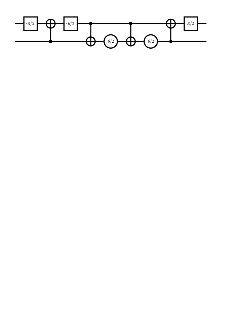
Figure 1: Quantum circuit realizing the gate $\textbf{G}(\theta)$. The Bell states of two qubits are its eigenstates. It shifts the phase of $\Phi^{+}$ state by $3\theta/4$ and the phases of the other three Bell states by $-\theta/4$. Two-qubit gates are CNOT gates, while one-qubit gates are rotations around $z$ (squares) or $y$ (circles) axis by the specified angle.

Other representations of AUEM for one qubit can be obtained by concatenating this circuit with a similar one applied to the qubits $X$ and $Y$ and with $\theta$ replaced by $\varphi-\varphi_{0}$ (see Fig. 2). For example, the asymmetric cloner AsymmClone may be realized in this way by putting $\varphi=0$.

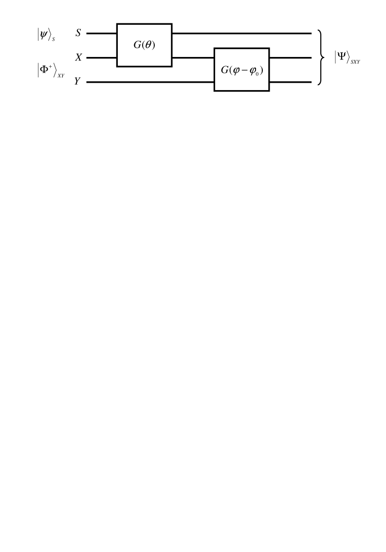
Figure 2: AUEM for one qubit. $S$ is the signal qubit in an unknown state. Qubits $X$ and $Y$ compose the 4-level ancilla and are initially prepared in the $\Phi^{+}$ Bell state. The gate $G(\theta)$ is shown in Fig. 1. The angles $\theta$ and $\varphi_{0}$ are connected to the fidelity $F$ by Eqs. (68), (64) with $d=2$. $\varphi$ is a free parameter. The output state is the pure entangled state of the three qubits.

The symmetric entangler, acting at the same time as the symmetric cloner and the universal-NOT gate, is realized by putting $\varphi=0$, $\theta=\arccos{(1/3)}$. The circuit depicted in Fig. 2 can be compared to the circuits suggested for the universal (symmetric) cloning machine UCMnetw , where both ancillary qubits interact with the signal. Our scheme has the advantage of minimizing the number of qubits involved into the interaction with the signal system.

V.2 Comparison with the symmetric entangler

The performance of the optimal AUEM for one qubit, can be compared to that of the symmetric entangler of Buz̆ek and Hillery SymmEnt . The symmetric entangler (see subsection IV.5) is a machine having two qubits as input, one of them being the signal qubit in an unknown state $\left|\psi\right>$ and another one being a specially prepared ancilla. The output of the machine is a pair of qubits in a mixed entangled state obtained from Eq. (61) by tracing out the system $X$:

$$\rho_{SY} = \frac{1}{6}\left(\left|\psi\right>\left|\psi^{\perp}\right>+\left|\psi^{\perp}\right>\left|\psi\right>\right)\left(\left<\psi\right|\left<\psi^{\perp}\right|+\left<\psi^{\perp}\right|\left<\psi\right|\right)$$ (74)

$$+\frac{2}{3}\left|\psi\right>\left|\psi\right>\left<\psi\right|\left<\psi\right|,$$

where the first vector in each pair of kets or bras is related to the signal qubit and the second one – to the ancillary qubit.

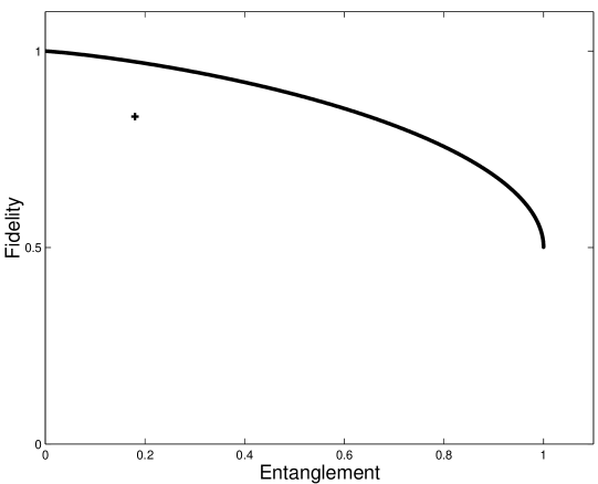
Figure 3: The output-to-input fidelity of the signal qubit as a function of the entanglement between the signal qubit and the ancilla, at the output of AUEM (solid line). The symmetric entangler of Ref. SymmEnt is shown by a cross.

Using the Wooters’ method WootersConc we calculate the amount of entanglement of formation contained in the output state, which is the upper bound for all other measures of entanglement. The concurrence of the state Eq. (74) is $C=\frac{1}{3}$ and the entanglement of formation is equal to $h_{2}\left(\frac{1}{2}(1+\sqrt{1-C^{2}})\right)\approx 0.19$ ebits. The output-to-input fidelity of the signal qubit can be easily found equal to $\frac{5}{6}$. These quantities can be compared to the corresponding quantities of the optimal AUEM. For the price of disturbance $\frac{1}{6}$ the AUEM produces $E=h_{2}(\frac{5}{6})=0.65$ ebits of entanglement, i.e. it is several times more effective than the symmetric entangler. It should be remembered also that the AUEM, in contrast to the symmetric entangler, allows us to vary the disturbance of the signal, finding the optimal trade-off between the fidelity and the entanglement (Fig. 3), which is very important for such applications as eavesdropping in quantum cryptography.

V.3 Application of AUEM to eavesdropping

Let us show that the optimal AUEM for one qubit realizes the interaction necessary for the optimal eavesdropping in the so-called six state protocol of quantum cryptography. In this protocol the value of a bit is encoded into the state of a qubit $S$, chosen from three bases: the “rectilinear” one, created by two orthonormal vectors $\left|0\right>$ and $\left|1\right>$, the “diagonal” one, created by

$$\left|\bar{0}\right>=\frac{1}{\sqrt{2}}\left(\left|0\right>+\left|1\right>\right),$$ (75)

$$\left|\bar{1}\right>=\frac{1}{\sqrt{2}}\left(\left|0\right>-\left|1\right>\right),$$ (76)

and the “circular” one:

$$\left|0^{\prime}\right>=\frac{1}{\sqrt{2}}\left(\left|0\right>+i\left|1\right>\right),$$ (77)

$$\left|1^{\prime}\right>=\frac{1}{\sqrt{2}}\left(\left|0\right>-i\left|1\right>\right).$$ (78)

The protocol of quantum key distribution is similar to BB84 BB84 , the only difference is that three bases are used instead of two. The advantage of this scheme over BB84, is that the former is more secure against the eavesdropping.

It has been shown 6state that the optimal strategy of individual eavesdropping to the six-state protocol is to attach to the qubit $S$ a 4-level ancilla in some state $\left|\chi\right>$ and to make the following transformation:

$$\left|0\right>\left|\chi\right>\longrightarrow\sqrt{F}\left|0\right>\left|A\right>+\sqrt{1-F}\left|1\right>\left|B\right>,$$ (79)

$$\left|1\right>\left|\chi\right>\longrightarrow\sqrt{F}\left|1\right>\left|C\right>+\sqrt{1-F}\left|0\right>\left|D\right>,$$ (80)

where $F$, as usual, is the channel fidelity for the qubit $S$, and the four states in the ancilla state space are chosen so that $\left\{\left|A\right>,\left|C\right>\right\}\perp\left|B\right>\perp\left|D\right>$, and $Re\left<A\right|\left.C\right>=2-1/F$.

If the optimal AUEM is used for entangling the qubit $S$ to the ancilla, we obtain from Eq. (53) for $d=2$:

$$\left|0\right>\left|\Phi^{+}\right>\longrightarrow\left|0\right>\left[\frac{\alpha+\beta}{\sqrt{2}}\left|0\right>\left|0\right>+\frac{\alpha}{\sqrt{2}}\left|1\right>\left|1\right>\right]$$

$$+\frac{\beta}{\sqrt{2}}\left|1\right>\left|1\right>\left|0\right>,$$ (81)

$$\left|1\right>\left|\Phi^{+}\right>\longrightarrow\left|1\right>\left[\frac{\alpha+\beta}{\sqrt{2}}\left|1\right>\left|1\right>+\frac{\alpha}{\sqrt{2}}\left|0\right>\left|0\right>\right]$$

$$+\frac{\beta}{\sqrt{2}}\left|0\right>\left|0\right>\left|1\right>,$$ (82)

where the kets are written in the $SXY$ order. It is straightforward to verify that the four states of ancilla entangled with the states of the qubit $S$ satisfy the demands imposed on the states $\left|A\right>$, $\left|B\right>$, $\left|C\right>$, $\left|D\right>$ for any value of $\varphi$. That is, the optimal AUEM can be used for optimal individual eavesdropping to the six state protocol of quantum cryptography. As we have seen, the entangling interaction can be designed in such way, that it comprise only two qubits of three, which may be a significant advantage in the practical applications of the eavesdropping techniques.

VI Conclusions

We have given a definition of asymmetric universal entangling machine for a $d$-level system and have proven its existence. We have shown that such a machine requires a $d^{2}$-level ancilla and have found the transformation producing maximal possible entanglement for a given degradation of the signal system fidelity. The obtained machine could also be called “depolarizing channel purificator”, since it realizes the most general unitary transformation of three $d$-level systems acting as a depolarizing channel in the state space of one of them. Thus, this machine represents a generic quantum model for studying various universal quantum processes.

It has turned out that this machine, AUEM, is a generalization to a wide variety of universal quantum machines suggested in the past years, comprising the symmetric and asymmetric quantum cloners, the symmetric quantum entangler, the UNOT gate and the quantum information distributor. All these devices are particular realizations of AUEM for a definite decomposition of the ancilla state space into direct product of state spaces of two $d$-level systems. This fact suggests that AUEM can be used in the same applications as the mentioned machines, having at the same time more degrees of freedom for tailoring the necessary interaction. Besides, it may find additional applications in quantum information procession with partially known states and in eavesdropping to various quantum cryptographic protocols.

The minimal-interaction representation of AUEM shows that for sufficiently high fidelity the entangling interaction requires a $d$-level ancilla only, instead of a $d^{2}$-level ancilla typically suggested. This result may simplify significantly the development of realistic universal quantum machines.

From the fundamental point of view, the present paper shows that the knowledge of quantum state is not necessary for entangling any quantum system to another system (which is itself in a known state). Thus, the famous Schrödinger’s gedankenexperiment can be modified in such a way that makes the initial state of the cat irrelevant. At the moment of box opening, the cat will be in a superposition of its initial state and all its other possible states life .

- (1) E. Schrödinger, Naturwiss. 23, 807 (1935).
- (2) For reviews on entanglement and quantum information see S. Ya. Kilin, Usp. Fiz. Nauk 169, 507 (1999) [Phys. Usp. 42, 435 (1999)]; S. Ya. Kilin, in Progress in Optics, ed. E. Wolf, 42, 1 (2001).
- (3) G. Alber, quant-ph/9907104.
- (4) V. Buz̆ek and M. Hillery, Phys. Rev. A 62, 022303 (2000).
- (5) M. Ricci, F. Sciarrino, C. Sias, and F. De Martini, Phys. Rev. Lett. 92, 047901 (2004); F. Sciarrino, F. De Martini, and V. Buz̆ek, quant-ph/0410224.
- (6) V. Buz̆ek and M. Hillery, Phys. Rev. A 54, 1844 (1996).
- (7) N. Gisin, S. Massar, Phys. Rev. Lett. 79, 2153 (1997); D. Bruss et al., Phys. Rev. A 57, 2368 (1998); D. Bruss, A. Ekert, and C. Macchiavello, Phys. Rev. Lett. 81, 2598 (1998).
- (8) V. Buz̆ek, S. L. Braunstein, M. Hillery, and D. Bruss, Phys. Rev. A 56, 3446 (1997); V. Buz̆ek, M. Hillery, and P. L. Knight, Fortschr. Phys. 46, 521 (1998).
- (9) V. Buz̆ek and M. Hillery, Phys. Rev. Lett. 81, 5003 (1998).
- (10) R. F. Werner, Phys. Rev. A 58, 1827 (1998); M. Keyl and R. F. Werner, J. Math. Phys. 40, 3283 (1999).
- (11) A. Lamas-Linares, C. Simon, J. C. Howell, and D. Bouwmeester, Science 296, 712 (2002); W. T. M. Irvine, A. Lamas-Linares, M. J. A. de Dood, and D. Bouwmeester, Phys. Rev. Lett. 92, 047902 (2004).
- (12) N. J. Cerf, Acta Phys. Slov. 48, 115 (1998); N. J. Cerf, Phys. Rev. Lett. 84, 4497 (2000); N. J. Cerf, J. Mod. Opt. 47, 187 (2000).
- (13) V. Buz̆ek, M. Hillery, and R. Bednik, Acta Phys. Slov. 48, 177 (1998); C.-S. Niu and R. B. Griffiths, Phys. Rev. A 58, 4377 (1998).
- (14) S. L. Braunstein, V. Buz̆ek, and M. Hillery, Phys. Rev. A 63, 052313 (2001).
- (15) V. Buz̆ek, M. Hillery, and R. F. Werner, Phys. Rev. A 60, 2626 (1999); N. Gisin and S. Popescu, Phys. Rev. Lett. 83, 432 (1999).
- (16) F. De Martini, V. Buz̆ek, F. Sciarrino, and C. Sias, Nature (London), 419, 815 (2002).
- (17) C. H. Bennet et al., Phys. Rev. A 53, 2046 (1996).
- (18) R. Josza, J. Mod. Opt. 41, 2315 (1994).
- (19) W. K. Wooters and W. H. Zurek, Nature (London) 299, 802 (1982).
- (20) G. M. D’Ariano and P. Lo Presti, Phys. Rev. A 64, 042308 (2001); V. Karimipour and A. T. Rezakhani, Phys. Rev. A 66, 052111 (2002).
- (21) C. H. Bennet et al., Phys. Rev. A 54, 3824 (1996).
- (22) M. Horodecki, P. Horodecki, and R. Horodecki, Phys. Rev. Lett. 84, 2014 (2000).
- (23) D. I. Fivel, Phys. Rev. Lett. 74, 835 (1995).
- (24) J. Preskill, Quantum information and computation. Lecture notes for Physics 229, California Institute of Technology (1998) (available at http://theory.caltech.edu/~ preskill/ph229/).
- (25) C. H. Bennett and G. Brassard, in Proceedings of IEEE International Conference on Computers, Systems and Signal Processing, Bangalore, India, 175 (IEEE, New York, 1984).
- (26) N. Gisin, G. Ribordy, W. Tittel, and H. Zbinden, Rev. Mod. Phys. 74, 145 (2002).
- (27) N. J. Cerf and S. Iblisdir, Phys. Rev. A 64, 032307 (2001).
- (28) R. Derka, V. Buz̆ek, and A. K. Ekert, Phys. Rev. Lett. 80, 1571 (1998).
- (29) W. K. Wooters, Phys. Rev. Lett. 80, 2245 (1998).
- (30) D. Bruss, Phys. Rev. Lett. 81, 3018 (1998).
- (31) Here we consider the states of alive and dead cat as different states in the state space of a very complicated but finite system. We do not discuss the problem of biological life description in the framework of quantum theory.