A Study on the Noise Threshold of Fault-tolerant Quantum Error Correction

Abstract

Quantum circuits implementing fault-tolerant quantum error correction (QEC) for the three qubit bit-flip code and five-qubit code are studied. To describe the effect of noise, we apply a model based on a generalized effective Hamiltonian where the system-environment interactions are taken into account by including stochastic fluctuating terms in the system Hamiltonian. This noise model enables us to investigate the effect of noise in quantum circuits under realistic device conditions and avoid strong assumptions such as maximal parallelism and weak storage errors. Noise thresholds of the QEC codes are calculated. In addition, the effects of imprecision in projective measurements, collective bath, fault-tolerant repetition protocols, and level of parallelism in circuit constructions on the threshold values are also studied with emphasis on determining the optimal design for the fault-tolerant QEC circuit. These results provide insights into the fault-tolerant QEC process as well as useful information for designing the optimal fault-tolerant QEC circuit for particular physical implementation of quantum computer.

I Introduction

Recent developments in the theory of quantum computation have generated significant interest in utilizing quantum mechanics to achieve new computational capability Nielsen and Chuang (2000). A quantum computer can outperform its classical counterpart and provide efficient ways to solve many important problems. However, the intrinsic sensitivity of a quantum superposition state to imperfect operations and interactions with its surrounding environment prohibits the realization of a scalable quantum computer. To combat the inevitable errors and decoherence of quantum states during the process of computation, quantum error correction (QEC) and fault-tolerant methods of quantum computation have to be applied in the construction of large-scale quantum computers. It has become clear that the future of robustly storing and manipulating quantum information rely upon the success of fault-tolerant quantum error correction Shor (1996); DiVincenzo and Shor (1996); Gottesman (1998).

Fault-tolerant methods combined with concatenated coding yield the threshold result, that states if the noise level per elementary operation is below a threshold value, then arbitrarily long quantum computation can be achieved using faulty components Zalka (1996); Aharonov and Ben-Or (1997); Knill et al. (1998); Preskill (1998). Using a $t$-error correcting code, fault-tolerant circuits constructed from faulty gates with error rate $\epsilon$ can achieve a logical error rate of $O(\epsilon^{t+1})$ per logical gate. This fact together with the concept of concatenated coding provide a method for possible large-scale quantum computation, and can lead to the realization of a scalable quantum computer. Therefore, it is important to study fault-tolerant methods and estimate the noise threshold values. In addition, the noise threshold indicates the tolerable noise level in a certain quantum circuit, and provides a benchmark for the efficiency of QEC circuits.

A number of theoretical estimates of noise threshold and improvements for the efficiency of QEC circuits have been proposed Zalka (1996); Aharonov and Ben-Or (1997); Knill et al. (1998); Preskill (1998); Steane (1999, 2003); Reichardt (2004); however, these studies adopt ad-hoc classical stochastic noise models that neglect device details, and make strong assumptions such as maximal parallelism and low noise level in storing qubits. Realistically, these assumptions are not usually applicable, and the power of fault-tolerant QEC under realistic physical conditions is still unclear. Noise threshold values are of little use if limitations of the physical implementation and realistic noise sources are not considered in the estimation. Therefore, it is of importance to study fault-tolerant QEC circuits using a noise model that reflects realistic device conditions.

In Ref. Cheng and Silbey (2004), we applied a phenomenological noise model to study the effect of noise in quantum teleportation and controlled-NOT gate operation. Starting from a effective system Hamiltonian that incorporates stochastic fluctuating terms to describe the effect of system-environment interactions, this model can describe the dissipative dynamics of a many-qubit system under realistic device conditions. In this paper, the same model is applied to investigate the performance of fault-tolerant QEC circuits implementing three qubit bit-flip code and five-qubit code. Relatively small codes are studied because we perform a systematic investigation on several variables that can affect the performance of fault-tolerant QEC circuits. In section II we first present the model Hamiltonian we used to implement quantum gates, and briefly review the noise model we proposed. We then introduce the fault-tolerant QEC circuits studied in this work in section III, and show our estimates of noise threshold in section IV. Finally, a systematic study on how factors like imperfect measurement, collective bath, repetition protocol, and level of parallelism affect the performance of fault-tolerant QEC is presented in section V. This theoretical study will be useful for the design and implementation of fault-tolerant QEC circuits. We briefly conclude our results in section VI.

II Interactions and Noise Model

We study the performance of fault-tolerant QEC circuits using a microscopic model described in Ref. Cheng and Silbey (2004). In this model, a qubit system is described by a Hamiltonian with a controlled part and a time dependent stochastic part. The general Hamiltonian of the qubit system can be written as ($\hbar=1$)

$$\begin{array}[]{rcl}\mathbf{H}(t)&=&\mathbf{H}_{0}(t)+\mathbf{h}(t),\end{array}$$ (1)

where the controlled Hamiltonian $\textbf{H}_{0}(t)$ describes the interactions between qubits, and the stochastic part $\textbf{h}(t)$ describes the fluctuations of the interactions due to the coupling to the environment. During the process of quantum computation, $\textbf{H}_{0}(t)$ is controlled to implement gate operations, whereas $\textbf{h}(t)$ is stochastic and results in the decoherence of the quantum system.

We choose to simulate fault-tolerant QEC circuits using a model control Hamiltonian with single-qubit $X$, $Z$ and two-qubit $ZZ$ interactions:

$$\mathbf{H}_{0}(t)={\displaystyle\sum_{i}\varepsilon_{i}(t)Z_{i}+}{\displaystyle\sum_{i}J_{i}(t)X_{i}}+{\displaystyle\sum_{i,j<i}g_{ij}(t)Z_{i}Z_{j},}$$ (2)

where $Z_{i}$ and $X_{i}$ are Pauli operators acting on the $i$-th qubit, and $\varepsilon_{i}(t)$, $J_{i}(t)$, and $g_{ij}(t)$ are controllable parameters that can be turn on and off to implement desired gate operations. For simplicity, all gate operations are simulated using step function pulses with field strengths set to 1 (uniform field strengths), and the “on-time” of each pulses are controlled to obtain the desired unitary transformations. Note that by doing so we adopt a dimensionless system in which a unit time scale $\Delta t$ is defined by the field strength $\varepsilon$, i.e. $\Delta t=1/\varepsilon$. We consider fault-tolerant QEC circuits composed only of single-qubit Hadamard gates, two-qubit controlled-NOT and controlled-Z gates, plus measurement of a single qubit in the computational basis. All these operations can be easily implemented using the model Hamiltonian in Eq. (2). Figure 1 shows the gate symbols and corresponding unitary transformations used in our simulations. Note that we adopt the $ZZ$ type two-qubit coupling in our model Hamiltonian for an illustrative purpose. The real form of the inter-qubit interaction depends on the controllable interactions available for each individual physical implementations. Nevertheless, our model can handle the other types of interactions as well, and we expect that the model Hamiltonian we use here can reproduce the same general physical behavior as other two-qubit Hamiltonians.

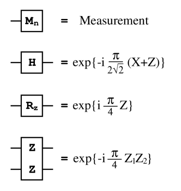
Figure 1: Quantum gate symbols used to denote unitary transformations implemented with single-qubit $X$, $Z$ and two-qubit $ZZ$ interactions. More complicated transformations such as controlled-NOT and controlled-Z gates can be trivially constructed using these elementary gates.

To describe the effect of noise, we consider fluctuations on the system Hamiltonian due to system-environment interactions:

$$\mathbf{h}(t)={\displaystyle\sum_{i}\delta\varepsilon_{i}(t)Z_{i}+}{\displaystyle\sum_{i}\delta J_{i}(t)X_{i}},$$

where $\delta\varepsilon_{i}(t)$ and $\delta J_{i}(t)$ describe the time-dependent diagonal and off-diagonal fluctuations on the $i$-th qubit, respectively. This corresponds to stochastic single-qubit phase ($Z)$ and bit-flip ($X$) errors on each individual qubit. In addition, we consider the fluctuations as random Gaussian Markov processes with zero mean and $\delta$-function correlation times described by the following set of equations:

$$\begin{array}[]{rcl}\langle\delta\varepsilon_{i}(t)\rangle&=&\langle\delta J_{i}(t)\rangle=0,\\ \langle\delta\varepsilon_{i}(t)\delta\varepsilon_{j}(t^{\prime})\rangle&=&\gamma_{0}\cdot\delta_{ij}\delta(t-t^{\prime}),\\ \langle\delta J_{i}(t)\delta J_{j}(t^{\prime})\rangle&=&\gamma_{1}\cdot\delta_{ij}\delta(t-t^{\prime}),\\ \langle\delta\varepsilon_{i}(t)\delta J_{j}(t^{\prime})\rangle&=&0,\end{array}$$ (3)

where bracket $\langle\rangle$ means averaging over the stochastic variables, and $\gamma_{0}$ and $\gamma_{1}$ describe the strength of the diagonal energy fluctuations and off-diagonal matrix element fluctuations, respectively. For a single-qubit system, $\gamma_{0}$ and $\gamma_{1}$ are well-defined physical quantities, i.e. $\gamma_{0}$ and $\gamma_{1}$ are population relaxation rate and pure dephasing rate, respectively Cheng and Silbey (2004). Note that noise strengths $\gamma_{0}$ and $\gamma_{1}$ should be interpreted as the error rate per unit time scale $\Delta t=1/\varepsilon$, where $\varepsilon$ is the strength of the control fields. Also notice that we treat the correlation between different qubits independently, which means each qubit in the system is coupled to a distinct environment (bath). Later we will remove this constraint and examine the effect of a collective bath on the noise threshold value. We also assume that the diagonal and off-diagonal fluctuations are not correlated.

For simplicity, we assume that the noise strengths are uniform, i.e. $\gamma_{0}$ and $\gamma_{1}$ are constants. The noise strength is set to be the same on all qubits at all times, therefore, we do not distinguish storage and gate errors. By assuming that the storage and gate errors are at the same level, the uniform noise assumption overestimates the errors in the system. At the same time it also avoids the weak storage noise assumption usually made in previous estimates of noise thresholds. Realistically, to perform a quantum gate between two distant qubits in a large-scale quantum circuit, multiple quantum swap gates must be employed to shuffle quantum states around Fowler et al. (2004). Our uniform noise assumption reflects the physical condition in this scenario. Note that more complex setups, in which control field and noise strengths are different for each individual qubits can be studied with exactly the same method.

Using the method described in Ref. Cheng and Silbey (2004) and Eq. (1)-(3), we can derive the equation of motion for the density matrix of the qubit system, and numerically propagate the density matrix of a system with up to twelve qubits (bound by the size of physical memory on a personal computer). This method provides an efficiently way to simulate quantum circuits and obtain full dynamics of the qubit system.

III Fault-Tolerant QEC Circuit

In this paper, we study fault-tolerant QEC circuits implementing the three qubit bit-flip code and five qubit code. We choose to investigate these two codes, because they are relatively small and allow us to perform systematic studies. Previous studies on the fault-tolerant QEC have been mainly focused on CSS codes, especially the CSS [[7,1,3]] code Calderbank and Shor (1996); Steane (1996, 1999). Because fault-tolerant encoded operations on CSS codes are easy to implement, CSS codes are expected to be more useful for quantum computation than the three qubit bit-flip code and five qubit code. Nevertheless, since we focus on variables affecting the performance of fault-tolerant QEC circuits, we expect that results gained in our study can be applied to more general codes. In this section, we introduce these two codes and the methods we apply to perform fault-tolerant QEC.

III.1 Fault-tolerant QEC scheme

We adopt the fault-tolerant QEC scheme proposed by DiVincenzo and Shor DiVincenzo and Shor (1996). This protocol utilizes cat states and transversal controlled-$X/Z$ gates to detect error syndromes. The procedure can be divided into three different stage: (1) ancilla preparation and verification, (2) syndrome detection, and (3) recovery.

To detect syndrome fault-tolerantly, ancilla qubits have to be prepared in maximally entangled cat states, and go through a verification step to ensure that magnitudes of correlated multiple-qubit errors are small. For example, the four-qubit cat state $\frac{1}{\sqrt{2}}(|0000\rangle+|1111\rangle)$ is necessary for the fault-tolerant QEC of the five-qubit code. Figure 2 shows the circuit we used to prepare and verify four-qubit cat states Preskill (1998). In this circuit, an extra qubit is used to detect correlated $X$ errors in the cat state; after the measurement, only states with measurement result equals to zero are accepted. This verification step ensures that a single-qubit error in the circuit causes at most a single-qubit error in the final cat state, therefore the circuit fulfills the fault-tolerant condition. Compared to other fault-tolerant cat state preparation circuits Nielsen and Chuang (2000); Steane (2004), an important feature in the circuit in Fig. 2 is that only a projective measurement is required to verify the cat state fault-tolerantly. This is possible because the circuit takes into account the error propagation pattern in the preparation step.

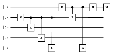
Figure 2: The fault-tolerant circuit for the preparation and verification of the four-qubit cat state. Note that the final result is conditioned by the outcome of the measurement at the end of the circuit. If the measurement outcome is zero, we accept the state; otherwise, the state is discarded and the circuit is started over again.

The ancilla cat state generated by the circuit presented in Fig. 2 is used to perform transversal controlled-stabilizer operation to transfer information about the errors from the data qubits to the ancilla qubits. After decoding the ancilla state, projective measurement is then applied to obtain error syndromes. Because there are more gates in the circuits than the number of measurements, it is reasonable to assume that measurement has smaller effect on the threshold result. Therefore, we assume perfect measurement. Later we will study the effect of measurement errors. In addition, to ensure that we do not accept a wrong syndrome, we must repeat syndrome detection and take a majority vote. Following Shor’s protocol, the following repetition scheme is used:

Repetition Protocol A (three majority vote):

1. Perform the syndrome detection twice. If the same measurement results are obtained, the syndrome is accepted and data qubits are corrected.

2. Otherwise, perform one more syndrome detection. If any two of the three measurement results are the same, the syndrome is accepted and data qubits are corrected.

3. If all three measurement results are different, no further action is taken.

This protocol is basically a simple majority vote in three trials. Note that the choice of the repetition protocol is not unique. In fact, later we will compare protocol A to another protocol, and show that we can improve this protocol to increase the efficiency of the fault-tolerant QEC procedure.

Combining all these elements, we can ensure that the probability of generating a two-qubit error is of order $\epsilon^{2}$, and avoid the catastrophic propagation of errors. During a quantum computation using a single-error correcting code, we can perform the fault-tolerant QEC after each gate operations. In consequence, single-qubit errors generated in earlier computation and QEC steps will be corrected in later QEC steps. Therefore, only two-qubit errors will be accumulated in a rate of order $\epsilon^{2}$. As a result, we can achieve longer computation when $\epsilon$ is small.

III.2 Three qubit bit-flip code

The three qubit bit-flip code encodes a logical qubit in three physical qubits using the following logical states:

$$\begin{array}[]{rcl}|0_{L}\rangle&=&|000\rangle,\\ |1_{L}\rangle&=&|111\rangle.\end{array}$$

This code is a stabilizer code with two stabilizer operators $g_{1}=ZZI$ and $g_{2}=IZZ$. The three qubit bit-flip code corrects single bit-flip error on any of the three data qubits. This code does not correct phase errors, therefore it is only useful when the degradation of the quantum state is dominated by bit-flip errors. However, we believe insights gained by studying this code can be applied to more general quantum error-correcting codes.

Figure 3 shows the syndrome detection circuit for the three qubit bit-flip code. In this circuit, physical qubits are depicted by horizontal solid lines, and quantum gates are represented by boxes. The quantum circuit includes three data qubits that take a encoded state as the input, and two pairs of ancilla qubits prepared in the Bell state $\frac{1}{\sqrt{2}}(|00\rangle+|11\rangle)$, which are used to measure the syndromes. We want to point out that only limited ability to perform operations in parallel is assumed in constructing this circuit. In addition, the circuit is arranged to minimize error propagation from the ancilla qubits to the data qubits. At the end of the circuit, two measurements, $M_{1}$ and $M_{2}$, are performed to obtain the error syndrome. After the syndrome is confirmed according to the repetition protocol A, we then apply the corresponding recovery action to correct the detected error. Table 1 lists the syndrome and the corresponding recovery actions for the three qubit bit-flip code.

Because the three qubit bit-flip code only corrects bit-flip errors, we only consider off-diagonal fluctuations on each qubit when dealing with this code ($\gamma_{0}=0$). Note that the circuit does not protect against $Z$ errors, nor can it prevent the generation of $Z$ errors. To access its performance on controlling $X$ errors on the data qubits, we only study the fault-tolerant QEC procedure when initially the data qubits are in the logical $|0_{L}\rangle$ state. This selection of initial state is unrealistic, but it allows us to avoid uncorrectable $Z$ errors that will ruin the QEC procedure.

Table 1: Measurement results and the corresponding actions required to correct the error in the data qubit for the three qubit bit-flip code.

Syndrome						Action
	M1	M2					UR
	0	0					III
	0	1					IIX
	1	0					XII
	1	1					IXI

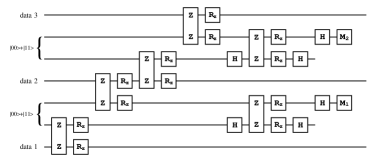
Figure 3: A circuit implementing the fault-tolerant syndrome detection for the three qubit bit-flip code.

III.3 The five-qubit code

The five-qubit code is the smallest quantum code that corrects all single-qubit errors Bennett et al. (1996); Laflamme et al. (1996). A scheme for fault-tolerant quantum computation using five-qubit code is presented by Gottesman in Ref. Gottesman (1998). Here we adopt the representation and fault-tolerant QEC circuit presented by DiVincenzo and Shor in Ref. DiVincenzo and Shor (1996). Their implementation uses a nine-qubit system with five data qubits and four ancilla qubits, which utilizes four-qubit cat state $\frac{1}{\sqrt{2}}(|0000\rangle+|1111\rangle)$ for syndrome detection. Moreover, four syndromes are detected sequentially. It is straightforward to simulate the syndrome detection circuit presented in their paper using our choice of model Hamiltonian (Eq. 1-3).

Ideally, multiple input states have to be studied to obtain averaged performance of the QEC procedure. To avoid such tedious computations, we use a logical qubit initially in the following pure state density matrix (in the $\{|0_{L}\rangle,|1_{L}\rangle\}$ basis):

$$\rho_{0}=\frac{1}{2}(I+\frac{1}{\sqrt{3}}X+\frac{1}{\sqrt{3}}Y+\frac{1}{\sqrt{3}}Z).$$

This state provides an averaged measure for all possible logical states, thus should give us a reasonable estimate of the averaged circuit performance.

Note that our setup simulates a minimal circuit for the fault-tolerant QEC using five-qubit code with limited physical resources. We expect such nine-qubit system can be realized on a liquid-state NMR quantum computer using available technologies. An experimental study on such minimal fault-tolerant QEC circuit will be an excellent test for our noise model, and can also provide us invaluable information that is essential for the design of large-scale quantum computers.

IV Estimate of Noise Threshold

To estimate the noise threshold for a logical operation, we simulate a computation where fault-tolerant QEC is performed after each logical operation on the encoded qubits, and compare the magnitude of logical errors to the magnitude of errors generated by the same operation on a bare physical qubit without QEC. We use the crash probability $P_{c}$ to describe the amount of logical errors in an encoded state. The crash probability is defined as the probability of having an uncorrectable error in the data qubits, and can be obtained from the fidelity of the state after a perfect QEC process.

We define a computational step as a logical gate followed by a fault-tolerant QEC step. If the same computational step is applied on the data qubits repeatedly $n$ times, we can describe the crash probability as a function of $n$, i.e. $P_{c}=P_{c}(n)$. In general, $P_{c}(n)$ satisfies an exponential form:

$$P_{c}(n)=\frac{1}{2}(1-e^{-2\Gamma_{n}n}).$$ (4)

We can perform simulation and compute crash probability at each step, $P_{c}(n)$. By fitting our simulation result to the functional form in Eq. (4), we obtain the crash rate constant per computational step $\Gamma_{n}=\left.\frac{dP_{c}(n)}{dn}\right|_{n=0}$. In addition, we also define the crash rate constant per unit time $\Gamma_{t}=\left.\frac{dP_{c}(t)}{dt}\right|_{t=0}=\Gamma_{n}/\tau$, where $\tau$ is the time period required to complete a computational step. Note that the unit time scale $\Delta t$ is defined by the strength of control fields $\varepsilon$, $\Delta t=1/\varepsilon$.

We compute noise threshold for a quantum memory, where repeated fault-tolerant QEC is applied on the data qubits to stabilize quantum information; and logical $X$ gate, where a logical $X$ gate followed by a fault-tolerant QEC step are applied on the data qubits. Figure 4 shows the crash rate constants as a function of noise strength for the three qubit bit-flip code, as well as the results for the five-qubit code. In Fig. 4, we clearly see that in the weak noise regime, the crash rate constant is proportional to the square of the noise strength, which reflects the power of the fault-tolerant QEC procedures. The noise threshold is obtained from the critical value where the crash rate constant for encoded computation cross over with the error rate of a bare physical qubit. At noise strength below the threshold value, the errors in the encoded state accumulated slower than for the bare physical qubit. At noise strength above the threshold value, the fault-tolerant QEC provides no benefit. For the three qubit bit-flip code, the noise threshold is about $2\times 10^{-2}$ for quantum memory, and about $1\times 10^{-3}$ for the logical $X$ gate.

We also perform calculations on five-qubit code. The five-qubit code corrects all single-qubit error, so we can compute the threshold for different types of noise. Table 2 summarizes threshold values for three qubit bit-flip code and five-qubit code. The difference in the noise threshold between quantum memory and logical $X$ gate is mainly due to the different basis of comparison. For the quantum memory, we need to compare crash rate constant per unit time $\Gamma_{t}$ to the decay rate of a free physical qubit; however, for the X gate, we need to use the crash rate constant per computational step $\Gamma_{n}$. The extra logical $X$ operation has little effect on the crash rate per computational step because the fault-tolerant QEC circuit is much bigger than the circuit for the logical $X$ gate. This observation suggests that other encoded single-qubit operations and transversal encoded two-qubit operations should have similar threshold values.

We summarize the assumptions we made for these calculations: (1) stochastic $X$ and $Z$ noises, (2) each qubit coupled to a distinct bath, (3) uniform noise strength, (4) perfect physical $|0\rangle$ states as initial states, (5) perfect instantaneous projective measurement. Clearly, the uniform noise assumption that treats gate errors and storage errors on the same footing is responsible for the relatively low threshold we obtain for the five-qubit code. In the next section we will examine some of these assumptions and discuss different factors that might affect the performance of fault-tolerant QEC.

Figure 4: Crash rate constants as a function of the noise strength. We show crash rate constants for a quantum memory using the three qubit bit-flip code (upper-left) and five-qubit code (upper-right), and for a logical $X$ gate on the three qubit bit-flip code (bottom-left) and on the five-qubit code (bottom-right). For the five-qubit code circuits, curves for different types of noise are presented. To show the threshold result, we also present curves for the error rate of a single physical qubit (dotted line). The noise threshold values are summarized in Table 2.

Table 2: Summary of noise threshold values. The noise strengths ($\gamma_{0}$ and $\gamma_{1}$) should be interpreted as the error rate per unit time scale $\Delta t=1/\varepsilon$, where $\varepsilon$ is the strength of the control fields.

		three qubit bit-flip code			five-qubit code
		quantum memory	X gate		quantum memory	X gate
$X$ errors ($\gamma_{1}$)		$2.1\times 10^{-2}$	$1.2\times 10^{-3}$		$4.2\times 10^{-4}$	$3.5\times 10^{-5}$
$Z$ errors ($\gamma_{0}$)		-	-		$5.1\times 10^{-4}$	$4.3\times 10^{-5}$
Both $X$ and $Z$ errors		-	-		$4.7\times 10^{-4}$	$3.9\times 10^{-5}$

V Efficiency of Fault-tolerant QEC Circuits

In this section, we study several variables that can affect the efficiency of the fault-tolerant QEC scheme. We perform a systematic investigation on the performance of quantum memories stabilized by fault-tolerant QEC and aim to generate a generic picture on how these variables change the efficiency of fault-tolerant QEC circuits.

V.1 Effect of imperfect measurement

We first test the effect of imperfect measurements on the performance of a quantum memory stabilized using fault-tolerant QEC. We use the following POVM (positive operator-valued measure) to describe an imperfect projective measurement on a single qubit:

$$\begin{array}[]{rcl}M_{0}&=&(1-\eta)|0\rangle\langle 0|+\eta|1\rangle\langle 1|,\\ M_{1}&=&(1-\eta)|1\rangle\langle 1|+\eta|0\rangle\langle 0|,\end{array}$$

where $M_{0}$ ($M_{1}$) describes events in which basis state $|0\rangle$ ($|1\rangle$) is measured, and $\eta$ is the probability of measurement error, i.e. a projection onto the wrong basis state. Figure 5 shows curves for the crash rate constant per unit time $\Gamma_{t}$ at different probabilities of measurement errors for a quantum memory implementing the three qubit bit-flip code. Clearly, $\Gamma_{t}$ is insensitive to the measurement errors even when the probability of measurement errors is significantly higher than the noise strength $\gamma_{1}$. The probability of the measurement error as high as 5% has only minor effect on the threshold value.

Figure 5: $\Gamma_{t}$ as a function of noise strength for the fault-tolerant QEC circuit using three qubit bit-flip code at different level of measurement errors. The error rate of a single physical qubit is also shown (dotted line). The measurement error has little effect on the threshold value.

V.2 Effect of a collective bath

A distinct feature of our noise model is the ability to describe the effect of a collective bath, in which all qubits are coupled to the same environment. Such an environment is relevant in physical implementations such as trapped-ion quantum computers, where qubits are coupled to the same collective phonon modes Cirac and Zoller (1995); Wineland et al. (2003). The effect of a collective bath on the fault-tolerant QEC is an interesting topic. Because a collective bath seems to contradict the idea of uncorrelated and stochastic errors that is the foundation of fault-tolerant QEC, several authors have suggested that collective decoherence has to be avoided for fault-tolerant quantum computing Preskill (1998); Steane (1998). Also, in a collective bath the effects of noise on different qubits add coherently; as a result, superdecoherence states exist, and might affect the efficiency of fault-tolerant QEC Palma et al. (1996).

To answer this question, we simulate the fault-tolerant QEC circuit for the three qubit bit-flip code using a noise model in which all qubits are coupled to a common bath. The following forms of correlation functions for the stochastic process are used:

$$\begin{array}[]{rcl}\langle\delta\varepsilon_{i}(t)\rangle&=&\langle\delta J_{i}(t)\rangle=0,\\ \langle\delta\varepsilon_{i}(t)\delta\varepsilon_{j}(t^{\prime})\rangle&=&\gamma_{0}\cdot\delta(t-t^{\prime}),\\ \langle\delta J_{i}(t)\delta J_{j}(t^{\prime})\rangle&=&\gamma_{1}\cdot\delta(t-t^{\prime}),\\ \langle\delta\varepsilon_{i}(t)\delta J_{j}(t^{\prime})\rangle&=&0,\end{array}$$ (5)

Notice that in Eq. (5), fluctuations on different qubits are fully correlated; this reflects the result of coupling to a common bath. Figure 6 shows the crash rate constant $\Gamma_{n}$ for quantum memories using the three qubit bit-flip code with two different types of baths. The crash rate curve for the collective bath case is only slightly higher than the curve for the localized bath, and there is no significant difference between these two lines. This result suggests that a collective Markovian bath, which exhibits spatial but not temporal correlation, has little effect on the efficiency of fault-tolerant QEC. Although superdecoherence states do exist when the system is coupled to a collective bath, they have little effect on the dynamics of the system, because those states represent only a small fraction in the whole Hilbert space. The fault-tolerant QEC circuit using the five-qubit code was also studied, and similar results were obtained.

Figure 6: The crash rate per computational step $\Gamma_{n}$ for the three qubit bit-flip code as a function of the noise strength. Curves for the distinct bath system (solid line) and collective bath system (dotted line) are shown. The result for the collective bath is close to the result for localized baths. This result suggests that collective bath has minor effect on the efficiency of fault-tolerant QEC.

V.3 Repetition protocol

Our simulation propagates the density matrix of the system in the process of computation, therefore, we obtain the full information about the time evolution of the system. By examining the trajectory of the system during the fault-tolerant QEC process, we find the following repetition protocol yields the best performance:

Repetition Protocol B (conditional generation):

1. Perform the syndrome detection once. If this syndrome is zero, do nothing.

2. Otherwise, perform the syndrome detection again. If the same syndrome is obtained, accept the syndrome and correct data qubits accordingly.

3. Otherwise, no further action is taken.

Figure 7 shows the crash rate constant $\Gamma_{n}$ for quantum memories implementing three qubit bit-flip code using different repetition protocols. Because the majority of the measured syndromes will be zero in the weak noise regime, protocol B reduces the amount of time required for a fault-tolerant QEC step by a factor of two. As a result, the crash rate constant per computational step $\Gamma_{n}$ decreases by a factor of two when protocol B is used. Similar improvements on the fault-tolerant QEC protocol have been suggested by other groups Plenio et al. (1997); Steane (2003); Reichardt (2004). The idea behind protocol B is that the syndrome detection circuit is complicated and generates extra errors on the data qubits, therefore minimizing the number of syndrome detection and accepting a syndrome only when two consecutive detections agree on the same syndrome improve the efficiency of the fault-tolerant QEC procedure.

Figure 7: The crash rate constant per step $\Gamma_{n}$ as a function of the noise strength for the two different repetition protocols for a quantum memory using three qubit bit-flip code. Using protocol B reduces the crash rate constant by a factor of two.

V.4 Level of parallelism

An important factor related to the efficiency of a QEC circuit is the level of parallelism in the circuit. The syndrome detection circuit shown in Fig. 3 is not optimized; for example, for a reasonable physical implementation, the first two controlled-Z gates might actually be operated in parallel to reduce the operation time. Figure 8 shows a compressed version of the syndrome detection circuit that has increased level of parallelism. Furthermore, because the interactions used to implement the controlled-Z gate commute with each other (Z and ZZ commute), the controlled-Z gate can be done in one step:

$$controlled-Z=e^{-i\pi Z_{1}Z_{2}/4}e^{i\pi(Z_{1}+Z_{2})/4}=e^{-i\pi(Z_{1}Z_{2}-Z_{1}-Z_{2})/4}.$$

This makes it possible to perform all controlled-Z operations in a single pulse. Note that this maximal parallelism design does not generally exist for arbitrary physical implementations, and is a special case for our choice of model interactions (ZZ coupling).

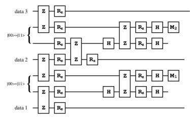
Figure 8: A circuit implementing the fault-tolerant syndrome detection for the three qubit bit-flipping code.

Figure 9 shows the crash rate constant per unit time $\Gamma_{t}$ for quantum memories implementing three qubit bit-flip code. Results for three syndrome detection circuits with different level of parallelism are shown. The noise thresholds for the original circuit (Fig. 3), increased parallelism circuit (8), and maximal parallelism circuit are about $1.5\times 10^{-2}$, $2.3\times 10^{-2}$, and $4.6\times 10^{-2}$, respectively. The results indicate that by increasing the level of parallelism, the noise threshold can be significantly improved. Note that the reduction of the operation time in higher level of parallelism can not account for all of the improvement on the threshold values; because the crash rate constant per unit time $\Gamma_{t}$ has been scaled by the amount of time needed to complete a fault-tolerant QEC step ($\Gamma_{t}=\Gamma_{n}/\tau$), any difference in $\Gamma_{t}$ is from sources other than difference in $\tau$. The improvement on the threshold value is due to the effect that when the level of parallelism is increased, the number of pathways that generate uncorrectable errors decreases. We emphasize that because our method of estimating noise threshold does not assume maximal parallelism, we can access the real threshold value that reflects the limitations of each individual physical implementations.

Figure 9: The crash rate constant per unit time $\Gamma_{t}$ as a function of the noise strength for quantum memories using three qubit bit-flip code. Curves for three syndrome detection circuits different in the level of parallelism are shown. The solid line is for the circuit shown in Fig. 3, the dashed line is the increased parallelism circuit shown in Fig. 8, and the dash-dotted line is the maximal parallelism circuit that finishes all controlled-Z operations in a single pulse. We see dramatic improvement on the noise threshold values when the level of parallelism is increased. The result indicates that by increasing the level of parallelism, the threshold value can be significantly improved.

VI Conclusion

We have applied a noise model based on a generalized effective Hamiltonian to study the effect of noise on the performance of fault-tolerant QEC circuits. The model includes realistic physical interactions for the implementations of quantum gates, and describes the effect of system-bath interactions by including stochastic fluctuating terms in the system Hamiltonian. As a result, this method simulates quantum circuits under physical device conditions, and gives us a full description of the dissipative dynamics of the quantum computer.

Fault-tolerant QEC circuits implementing either the three qubit bit-flip code or the five-qubit code were investigated, and the noise threshold for quantum memory and logical $X$ gate were calculated by comparing the logical crash rate to the error rate of a bare physical qubit. The noise threshold of quantum memories using the three qubit bit-flip code and five qubit code is about $2\times 10^{-2}$ and $5\times 10^{-4}$, respectively. The noise threshold of logical $X$ gates using the three qubit bit-flip code and five qubit code is about $1\times 10^{-3}$ and $4\times 10^{-5}$, respectively. Note that in our dimensionless system, these noise strength values should be interpreted as the error rate per unit time scale $\Delta t=1/\varepsilon$, where $\varepsilon$ is the strength of the control fields. These threshold values are obtained from an uniform noise model where magnitudes of storage errors and gate errors are the same. This result indicates that fault-tolerant quantum computing is possible in systems with strong storage errors. A possible scenario for such system is the linear nearest-neighbor architecture, where only nearest-neighbor interactions are available for two-qubit gates, and excess amount of quantum swap gates have to be added to the circuit to perform two-qubit gates between qubits distant in space.

We have also carried out a systematic study on several variables that can affect the performance of the fault-tolerant QEC procedure for the three qubit bit-flip code. Our results show that both collective bath and imperfect projective measurement have minor effects on the threshold value. However, the repetition protocol and level of parallelism can significantly change the performance of the fault-tolerant QEC procedure. Our density matrix results indicate that accepting a syndrome only when two consecutive syndrome detections agree (protocol B), which reduces the number of required syndrome detection steps, is the optimal repetition protocol. Compared to the simple majority vote algorithm (protocol A), protocol B increases the efficiency of fault-tolerant QEC at least by a factor of two. Regarding the level of parallelism in the syndrome detection circuit, in general, a higher level of parallelism results in a more efficient fault-tolerant QEC circuit. The improvement can not be fully explained by the shorter operational time for a more parallelized circuit; we suggest the major contribution for the improvement comes from the reduction of possible pathways for error propagation. Since the level of parallelism is actually limited by available physical resources in reality, it will be interesting to examine and simulate this factor according to a specific physical implementation of quantum computer (such as ion-trap or NMR).

Finally, we emphasize that without specifying the specific noise model and physical device conditions, noise threshold values are of little usefulness. Our noise model is based on well defined parameters that reflect realistic device conditions, and provides a full description for the dissipative dynamics of the quantum computer. As a result, this noise model enables us to access the real performance of fault-tolerant QEC for individual physical implementations. We believe that such information can be useful for the design and optimization of quantum computers.

References

- Nielsen and Chuang (2000) M. Nielsen and I. Chuang, Quantum Computation and Quantum Information (Cambridge University Press, 2000).
- Shor (1996) P. W. Shor, in Proceedings of the 37th Symposium on Foundations of Computer Science (IEEE Computer Society Press, Los Alamitos, CA, 1996), p. 56.
- DiVincenzo and Shor (1996) D. DiVincenzo and P. Shor, Phys. Rev. Lett. 77, 3260 (1996).
- Gottesman (1998) D. Gottesman, Phys. Rev. A 57, 127 (1998).
- Zalka (1996) C. Zalka, e-print quant-ph/9612028 (1996).
- Aharonov and Ben-Or (1997) D. Aharonov and M. Ben-Or, in Proceedings of the twenty-ninth annual ACM symposium on Theory of computing (ACM Press, 1997), pp. 176–188, ISBN 0-89791-888-6.
- Knill et al. (1998) E. Knill, R. Laflamme, and W. Zurek, Proc. R. Soc. London A 454, 365 (1998).
- Preskill (1998) J. Preskill, Proc. R. Soc. London A 454, 385 (1998).
- Steane (1999) A. Steane, Nature 399, 124 (1999).
- Steane (2003) A. Steane, Phys. Rev. A 68, 042322 (2003).
- Reichardt (2004) B. W. Reichardt, e-print quant-ph/0406025 (2004).
- Cheng and Silbey (2004) Y. Cheng and R. Silbey, Phys. Rev. A 69, 052325 (2004).
- Fowler et al. (2004) A. Fowler, C. Hill, and L. Hollenberg, Phys. Rev. A 69, 042314 (2004).
- Calderbank and Shor (1996) A. Calderbank and P. Shor, Phys. Rev. A 54, 1098 (1996).
- Steane (1996) A. Steane, Phys. Rev. Lett. 77, 793 (1996).
- Steane (2004) A. M. Steane, e-print quant-ph/0202036 (2004).
- Bennett et al. (1996) C. Bennett, D. DiVincenzo, J. Smolin, and W. Wootters, Phys. Rev. A 54, 3824 (1996).
- Laflamme et al. (1996) R. Laflamme, C. Miquel, J. Paz, and W. Zurek, Phys. Rev. Lett. 77, 198 (1996).
- Cirac and Zoller (1995) J. Cirac and P. Zoller, Phys. Rev. Lett. 74, 4091 (1995).
- Wineland et al. (2003) D. Wineland, M. Barrett, J. Britton, J. Chiaverini, B. DeMarco, W. Itano, B. Jelenkovic, C. Langer, D. Leibfried, V. Meyer, et al., Philos. Trans. R. Soc. Lond. Ser. A-Math. Phys. Eng. Sci. 361, 1349 (2003).
- Steane (1998) A. Steane, Fortschritte Phys.-Prog. Phys. 46, 443 (1998).
- Palma et al. (1996) G. Palma, K.-A. Suominen, and A. Ekert, Proc. R. Soc. Lond. A. 452, 567 (1996).
- Plenio et al. (1997) M. Plenio, V. Vedral, and P. Knight, Phys. Rev. A 55, 4593 (1997).