Entanglement and its Role in Shor’s Algorithm

Abstract

Entanglement has been termed a critical resource for quantum information processing and is thought to be the reason that certain quantum algorithms, such as Shor’s factoring algorithm, can achieve exponentially better performance than their classical counterparts. The nature of this resource is still not fully understood: here we use numerical simulation to investigate how entanglement between register qubits varies as Shor’s algorithm is run on a quantum computer. The shifting patterns in the entanglement are found to relate to the choice of basis for the quantum Fourier transform.

,

1 Introduction

Quantum computation has the potential to provide significantly more powerful computers than classical computation – if we can build them. There are numerous possible routes forward for quantum hardware [1], however, progress in the development of algorithms has been slow, in part because we don’t yet fully understand how the quantum advantage works. There are two key characteristics of the quantum resources used for computation. The first is that a general superposition of $2^{n}$ levels may be represented in $n$ 2-level systems [2], allowing the the physical resource to grow only linearly with $n$ (quantum parallelism). The second aspect is best explained by considering the classical computational cost of simulating a typical step in a quantum computation. If entanglement is absent then the algorithm can be simulated with an equivalent amount of classical resources. Jozsa and Linden [3] showed that, if a quantum algorithm cannot be simulated classically using resources only polynomial in the size of the input data, then it will have multipartite entanglement involving unboundedly many of its qubits – if it is run on a quantum computer using pure quantum states. However, the presence of multipartite entanglement is not a sufficient condition for a pure state quantum computer to be hard to simulate classically. As Jozsa and Linden point out, if the quantum computer is described using stabilizer formalism [4, 5], there are many highly entangled states that have simple classical descriptions. Moreover, a quantum computer using mixed states may still require exponential classical resources to simulate even if its qubits are not entangled, and it is not known whether such states may be used to perform efficient computation. In any case, being hard to simulate classically doesn’t imply the quantum process is doing any useful computation. If we want to understand quantum computation, we will have to look more closely at specific examples.

Few quantum algorithms provide an exponential speed up over classical algorithms, of those that do, Shor’s algorithm (order-finding) [6] is perhaps the most important because it can be used to factor large numbers and hence has implications for classical security methods. There is no proof that an equally efficient classical algorithm cannot exist for Shor’s algorithm, and it is worth noting that a sub-exponential algorithm has been found recently for the related problem of primality testing [7]. Proving a speed up is in general a tough task, few such proofs exist for exponential speed up of quantum over classical, one example being a quantum walk algorithm with a proven exponential speed up (w.r.t. an oracle) [8].

Assuming that Shor’s algorithm does provide an exponential speed up, and given that multipartite entanglement is necessary (though not sufficient) for pure state quantum computation with an exponential speed up over classical computation, in this paper we investigate what the entanglement is doing during the computational process, as it proceeds, gate by gate. To be clear, we reiterate that we are not trying to prove whether entanglement is present, we take it as given that there will be at least $\log r$ of entanglement entropy (where $r$ is the period being determined, and logs are in base 2 throughout this paper) at the mid-point of Shor’s algorithm, as first shown by Nielsen and Chuang [9]. Instead, we would like to know what role it plays in the computation. What we have in mind is a role comparable to the role of entanglement in quantum communications, where a maximally entangled pair of qubits can be used to perform specific communications tasks (such as teleportation of an unknown quantum state [10], or transmission of two classical bits of information [11]), which consume the entanglement in direct proportion to the amount of communication achieved. To date, little has been said about what role entanglement actually plays in quantum computation, the focus has been almost entirely on proving it is present, in sufficient quantities to make classical simulation inefficient (besides [3], see, for example, [12, 13, 14, 15]). We aim to throw some light on the question of what function it plays by calculating the entanglement as it varies during the course of the execution of Shor’s algorithm, and looking at how it correlates with the progress of the algorithm.

For this study, we are using a standard gate sequence for Shor’s algorithm using pure quantum states. Use of mixed states and different gate sequences may produce different entanglement patterns, but if there is a crucial role for entanglement in the computation, it will be identifiable as a common feature of all implementations. Parker and Plenio [16] have presented a version of Shor’s algorithm using only one pure qubit, the rest may start in any mixed state. They confirmed (numerically) that entanglement was present when the algorithm ran efficiently for factoring 15 and 21.

We should also add that, since we are investigating the logical functioning of the algorithm, we are not concerned with any practical questions of imperfect gates, decoherence, etc., nor with optimising the gate sequences given constraints on the number of qubits or the types of gates available. Much valuable work has been done in these areas by many authors, notably Vedral et al, [17], Gossett [18], and Van Meter and Itoh [19] on constructing efficient operations from elementary gates; Zalka [20] and Beauregard [21] who optimise the overall operation of Shor’s algorithm in fewer qubits; and Fowler and Hollenberg [22] who analyse scalability and accuracy.

The organisation of this paper is as follows. We start with a brief overview of Shor’s algorithm in §2, to set up our notation. This is followed in §3 by a discussion of how the entanglement varies in an instance of factoring 15, which also serves to introduce the entanglement measures we are using. In §4 the pattern of entanglement in several examples of factoring 21 is presented. Larger semiprimes are tackled in §5, from which we are able to deduce our main conclusions, which are summarised in §6.

2 Shor’s Algorithm

We begin with a brief overview of how Shor’s algorithm works, in order to remind the reader and to establish our notation. We wish to factor a number $N=pq$ where $p$ and $q$ are prime numbers. Classical number theory provides a way to determine these primes with high probability (not unity generally) by finding the period $r$ of the function

$$f_{x}(a)=x^{a}(\text{mod $N$}),$$ (1)

where $x$ is an integer chosen to be less than $N$ and co-prime to it, and $a\in\mathbb{Z}$. It is efficient to check whether $x$ is co-prime to $N$ using Euclid’s algorithm [23]. If $x$ happens not to be co-prime then their common factor gives a factor of $N$ and the job is done, but this happens only rarely for large $N$. Once the period $r$ is found, the numbers

$$m_{\pm}=x^{r/2}\pm 1$$ (2)

generally share either $p$ or $q$ with $N$ as a common factor. Not all choices of $x$ give periods $r$ which yields a factor $p$ or $q$. For instance, sometimes the period $r$ will be odd, whence the numbers from eq. (2) can be non-integer. When the chosen $x$ does not lead to a valid factor, the procedure can be repeated with a different choice until a factor is found. This is efficient since the probability of success is at least $\frac{1}{2}$ per trial for the case of semiprimes (see Shor [6]).

The hard part of the algorithm is determining the period $r$ of the function $f_{x}(a)=x^{a}(\text{mod $N$})$. Shor found a very elegant and efficient means of doing this quantum mechanically, depicted schematically in fig. 1.

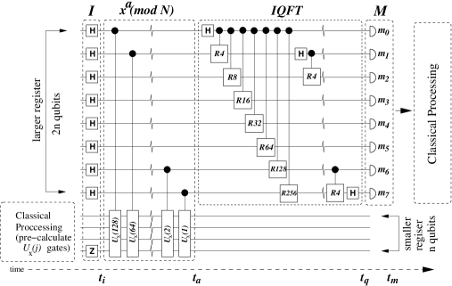
Figure 1: Schematic circuit diagram of Shor’s algorithm for factoring 15 implemented on a 12 qubit quantum register. The initialisation $I$ is done with single qubit Hadamard (H) and bit-flip (Z) gates. Controlled-$U_{x}(j)$ gates are used to produce $x^{a}(\text{mod $N$})$. The inverse quantum Fourier transform (IQFT) uses controlled rotations ($Rm$). The last quantum step is the measurement (M), which is followed by classical post-processing to obtain a factor of $N$.

Consider that one has two quantum registers (one of size $2n$ where $n=\lceil\log N\rceil$ qubits and the second of size $n$ qubits. We will denote the basis states of a quantum register by $|a\rangle$, with $a\in\{0\dots 2^{2n}-1\}$. The binary representation of $a$ indicates which register qubits are in the state representing zero and which are in the state representing one. A general state of a $2n$ qubit register $|\psi(t)\rangle$ at time $t$ can thus be written as a superposition of basis states,

$$|\psi(t)\rangle=\sum_{a=0}^{2^{2n}-1}\alpha_{a}(t)|a\rangle,$$ (3)

where $\alpha_{a}(t)$ is a complex number, normalised such that $\sum_{a=0}^{2^{2n}-1}|\alpha_{a}(t)|^{2}=1$. The algorithm begins by preparing the larger quantum register in an equal superposition $(2^{2n})^{-1/2}\sum_{a=0}^{2^{2n}-1}|a\rangle$ of all possible $2^{2n}$ basis states while the smaller register is prepared in the definite state $|1\rangle$ ($\equiv|0\dots 01\rangle$). The initial state of both registers is thus

$$|\Psi(t_{i})\rangle=\frac{1}{2^{n}}\sum_{a=0}^{2^{2n}-1}|a\rangle|1\rangle$$ (4)

The next step is a unitary transformation which acts on both registers according to $U|a\rangle|b\rangle=|a\rangle|bx^{a}(\text{mod $N$})\rangle$ giving the output state

$$|\Psi(t_{a})\rangle=\frac{1}{2^{n}}\sum_{a=0}^{2^{2n}-1}|a\rangle|x^{a}(\text{mod $N$})\rangle$$ (5)

Then an inverse quantum Fourier transform (IQFT) defined by

$$Q^{-1}|y\rangle=\frac{1}{2^{n}}\sum_{z=0}^{2^{2n}-1}\e^{-2\pi iyz/2^{2n}}|z\rangle$$ (6)

is applied, which transform the state $|\Psi(t_{a})\rangle$ from eq. (5) into

$$|\Psi(t_{q})\rangle=\frac{1}{2^{2n}}\sum_{a=0}^{2^{2n}-1}\sum_{z=0}^{2^{2n}-1}\e^{-2\pi iaz/2^{2n}}|z\rangle|x^{a}(\text{mod $N$})\rangle.$$ (7)

By measuring the larger register in the computational basis we obtain an integer number $c$. Now $c/2^{2n}$ is a close approximation to the fraction $k/r$, where $0\leq k<r$, the value of $k$ varies depending on the particular value of $c$ that is measured, but both $r$ and $k$ can be obtained classically using continued fractions (provided $c\neq 0$). Choosing the larger register to be $2n$ qubits provides a high enough accuracy for $c$ such that $r$ can be determined from a single measurement on all $2n$ qubits. It is possible to use fewer qubits in this first register but the probability of correctly determining $r$ decreases, and the algorithm may need to be repeated correspondingly many more times. If $r$ is not prime, and happens to share a factor $p$ with $k$, then one also fails to determine $r$ correctly, instead obtaining $r/p$. Again, this only reduces the probability of success by a factor polynomial in $N$, so the exponential nature of the speed up is maintained.

3 Factoring 15

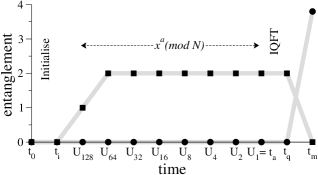
Figure 2: Entanglement between the two registers (squares) and within the smaller register (circles) in Shor’s 12 qubit algorithm as a function of gates sequence according to fig (1) with the co-prime chosen as $x=13$. The entanglement within the larger register is zero throughout.

We start our analysis of the entanglement by studying the circuit for factoring 15 (3x5), though it is not necessarily typical of factoring larger numbers. Since many gates make no change to the entanglement, rather than tracking the entanglement as each basic gate is applied, we choose to look at certain key points in the algorithm. We restrict our attention to controlled composite gates: the $U_{x}(j)$ gate which implements the operation $x^{j}(\text{mod $N$})$ for $j\in\{1,2,4\dots 2^{2n}\}$, and the rotations in the IQFT. Details of how to efficiently construct these composite gates from a universal set of one and two qubit gates may be found in, for example, [4]. There are 8 of the $U_{x}(j)$ gates (in general $2n$, one for each larger register qubit), which is manageable, but for the IQFT there are 27 (in general $(2n+1)(n-1)$ for a $2n$ qubit register) rotation gates: for our purposes in this paper it is sufficient to treat the whole IQFT as one unit. Along with single qubit gates as necessary, the circuit using these composite gates is depicted in fig. 1.

As we are only considering the evolution of pure states we can measure the entanglement between the two registers using the entropy of the subsystems

$$E_{c}=-\sum_{i}\lambda_{i}\log\lambda_{i},$$ (8)

where the $\{\lambda_{i}\}$ are the eigenvalues of the reduced density matrix of either of the registers (both have the same eigenvalues). The reduced density matrix of one of the registers is obtained from the full pure state of the system by applying a partial trace over the other register,

$$\rho_{L}(t)=\text{Tr}_{S}|\Psi(t)\rangle\langle\Psi(t)|,$$ (9)

and similarly $\rho_{S}(t)=\text{Tr}_{L}|\Psi(t)\rangle\langle\Psi(t)|$, where $L$ and $S$ denote the larger and smaller registers respectively.

To quantify the entanglement within each register is not so straightforward. Most entanglement measures for mixed states, such as $\rho_{L}$ and $\rho_{S}$, are computationally intractable in practice for more than a few qubits; we also need to consider all the possible divisions of the qubits into different subsets in order to locate all of the entanglement. A reasonable approximation to quantifying the entanglement within a register can be obtained by applying a partial transpose to each possible subset of qubits and calculating the negativity [24, 25] given by $\eta=\text{Tr}|\rho^{T}|-1$ i.e., the sum of the negative eigenvalues of the transposed matrix $\rho_{L}^{T}$ or $\rho_{S}^{T}$. If the negativity is zero for all possible subsets of qubits in the register, then we can say that at most the register has bound entanglement [26], which is not generally considered useful for quantum information tasks (though see [27]). Non-zero negativity for any subset of qubits definitely indicates the presence of entanglement (across that particular division).

Finally, we use the entanglement of formation [28] to quantify the pairwise entanglement between two qubits. The entanglement of formation quantifies how much entanglement is needed to make the state from unentangled ingredients. In general it is hard to calculate explicitly, however, Wootters [28] found an elegant formula for the case of two qubits in a mixed state $\rho$, the concurrence $C$ is given by $C=\text{max}(\lambda_{1}-\lambda_{2}-\lambda_{3}-\lambda_{4},0)$, where the $\lambda_{i}$ are the square roots of the eigenvalues of $\rho\tilde{\rho}=\rho\;\sigma_{y}^{A}\!\otimes\!\sigma_{y}^{B}\rho^{*}\sigma_{y}^{A}\!\otimes\!\sigma_{y}^{B}$, with $A$, $B$ labels for the two qubits, $\sigma_{y}$ the Pauli spin operator, and $\rho^{*}$ denotes the complex conjugation of $\rho$ in the computational basis $\{|00\rangle,|01\rangle,|10\rangle,|11\rangle\}$. The entanglement of formation $E_{f}=h(\frac{1}{2}+\frac{1}{2}\sqrt{1-C^{2}})$, where $h(\eta)$ is the binary entropy function, $h(\eta)=-\eta\log(\eta)-(1-\eta)\log(1-\eta)$. We use $E_{f}$ to check for pairwise entanglement within and between the qubit registers. Note that quantum states can be highly entangled even without containing any pairwise entanglement [29, 30].

In fig. 2 we plot the entanglement in Shor’s algorithm using the entropy of the subsystem where possible (full state is pure) and the negativity where the single register state is mixed. The negativity turns out to be zero for both registers throughout the algorithm (except the measurement leaves the smaller register entangled, but this cannot be useful for the remaining classical steps of the algorithm). The entanglement between the registers builds up to a maximum during the first two $U_{x}(j)$ gates, then stays constant until the measurement. We also note (from calculating the entanglement of formation for appropriate pairs of qubits) that there is no pairwise entanglement between any pair of qubits at any of the sampled points in this instance of the algorithm, neither within nor between the registers.

Since the IQFT is the crucial step for finding the period, we looked in more detail at how the distribution of the entanglement changes over the operation of the IQFT.

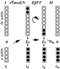
Figure 3: Pattern of entanglement during Shor’s algorithm factoring $N=15$ with co-prime $x=13$. After the $U_{x}(j)$ gates the top two qubits in the larger register (filled) are entangled with the four qubits in the smaller register. After the IQFT, the entanglement is transfered to the lower two qubits in the larger register. Qubits represented by open circles are not entangled. Time sequence corresponds to fig. 1.

Unitary operations can only alter entanglement within the elements they are applied to. Applying this principle to the circuit in fig. 1, since the entanglement within each register is zero (strictly speaking, zero apart from possible bound entanglement) after the modular exponentiation, it is clear that entanglement cannot decrease during the IQFT, since no further gates act where the only significant entanglement is located, between both registers. Furthermore, since each pair of qubits in the upper register has an entangling (2-qubit) gate applied to it only once during the algorithm, entanglement within the upper register can only be generated or shifted around, not decreased. And indeed our numerical calculations show the distribution of entanglement between the individual qubits does change in our example of factoring 15 with $x=13$. By examining the entropy of each possible subset of qubits in each register, we can deduce that only two of the eight qubits are entangled with the four qubits in the smaller register, and during the action of the IQFT, this entanglement is transfered from the top two qubits to the bottom two in the larger register. We represent this schematically in fig. 3.

However, we should remember that 15 is actually extremely easy to factor. It is straightforward to see that at least one of $x^{r/2}\pm 1$ is divisible by 3 or 5 for almost any random choice of $x,r>1$, regardless of whether $x$ is co-prime to $N$ or whether $r$ is the period of $x^{a}(\text{mod $N$})$. To learn anything significant, we need to look at more examples.

4 Factoring 21

Table 1: Average entropy of subsystems for factoring 21 with $x=2$, and average negativity (after the IQFT) for different sized subsystems of the larger register.

size of		large register		large register	large register
subsystem	small register	after $U$	after IQFT	difference $\Delta E_{1}$	negativity
1 qubit	0.811	1.000	0.938	-0.062	0.172
2 qubits	1.538	1.600	1.599	-0.001	0.397
3 qubits	2.151	1.843	2.020	+0.177	0.591
4 qubits	2.585	1.972	2.283	+0.311	0.678
5 qubits	2.585	2.081	2.447	+0.366	0.749
6 qubits		2.184	2.547	+0.363
7 qubits		2.285	2.602	+0.318
8 qubits		2.385	2.589	+0.204
9 qubits		2.485	2.619	+0.134

We next look at factoring 21 ($3\times 7$). To do this on a quantum computer in the same manner as the circuit for factoring 15 shown in fig. 1 requires a total of 15 qubits, 10 in the larger register and 5 in the smaller. For co-prime $x=13$, we find a similar pattern of entanglement to that shown in fig. 3 for 15 with $x=13$, except that for 21 there is only entanglement between one qubit in the larger register and two qubits in the lower register. Similarly, the IQFT step shifts the entanglement from the top qubit to the bottom qubit in the larger register. Again, there is no pairwise entanglement, so the three entangled qubits are in a GHZ type of state [31], i.e., one that can be rotated into the form $\alpha|000\rangle\pm\beta|111\rangle$.

The larger register is now at the limit of our computational resources for calculating the full analysis of the negativity. Instead of calculating the negativity for all possible subsets of qubits in a register, we used randomly sampled subsets, from which we deduce that with high probability for co-prime $x=13$ there is no entanglement within either register at any stage of the algorithm. For other choices of co-prime such as $x=2$ and $x=4$, there is no entanglement within either register by the end of the modular exponentiation ($U_{x}(j)$ gates), but entanglement is generated within the larger register during the IQFT. For these co-primes we also find a more complex pattern in the entropies of the subsystems: the entanglement now involves all of the register qubits. The details for $x=2$ are shown in table 1. Essentially the entanglement becomes more multipartite: the average entropy reduces slightly for one and two qubit subsets, while for larger subsets it increases. Examination of the entanglement of formation for pairs of qubits taken one in each register shows there is also a significant amount of pairwise entanglement (average 0.261 per pair before the IQFT) contributing to the total entanglement in the system. The average pairwise entanglement of formation between the registers decreases slightly (from 0.261 to 0.242) after the IQFT. This change is possible because entangling gates on the upper register can convert the pairwise entanglement into something more multipartite involving more than two of the upper register qubits. We will discuss what these entanglement patterns can tell us in the next section after we examine larger examples.

5 Factoring larger numbers

In order to examine examples with prime factors larger than 3 or 5, we pushed our numerical studies as far as we could with this gate model, by analysing semiprimes $32<N<64$ and $64<N<128$, which require 18 and 21 qubits respectively for the quantum registers. In these cases, though we cannot easily calculate a full entanglement analysis, we have calculated the entropy between one qubit and the rest of the qubits in both registers, this corresponds to the quantities in the third and fourth columns in the top line of table 1. The difference in the average entropy $\Delta E_{1}$ before and after the IQFT (corresponding to the first entry in the fifth column in table 1), is shown in table 2 grouped by the period $r$, as a total for the whole upper register (so the entry for $N=21$, $r=6$ is $0.624=10\times 0.062$ from table 1).

Table 2: Average decrease in entanglement $-\langle\Delta E_{1}\rangle$ between one qubit and the rest during the IQFT step (total for upper register, see text for details).

$N$	$r$ (number of co-primes with this $r$)
$p\times q$	$-\langle\Delta E_{1}\rangle$
$15$	2 (3)	4 (4)
$3\times 5$	0.0	0.0
$21$	2 (3)	3 (2)	6 (6)
$3\times 7$	0.0	0.706	0.624
$33$	2 (3)	5 (4)	10 (12)
$3\times 11$	0.0	0.285	0.256
$35$	2 (3)	3 (2)	4 (4)	6 (6)	12 (8)
$5\times 7$	0.0	0.869	0.0	0.788	0.706
$39$	2 (3)	3 (2)	4 (4)	6 (6)	12 (8)
$3\times 13$	0.0	0.869	0.0	0.788	0.706
$51$	2 (3)	4 (4)	8 (8)	16 (16)
$3\times 17$	0.0	0.0	0.0	0.0
$55$	2 (3)	4 (4)	5 (4)	10 (12)	20 (16)
$5\times 11$	0.0	0.0	0.285	0.256	0.226
$57$	2 (3)	3 (2)	6 (6)	9 (6)	18 (18)
$3\times 19$	0.0	0.869	0.788	0.080	0.071
$77$	2 (3)	3 (2)	5 (4)	6 (6)	10 (12)	15 (8)	30 (24)
$7\times 11$	0.0	1.033	0.343	0.951	0.314	0.034	0.031
$91$	2 (3)	3 (8)	4 (4)	6 (24)	12 (32)
$7\times 13$	0.0	1.033	0.0	0.951	0.869
$119$	2 (3)	3 (2)	4 (4)	6 (6)	8 (8)	12 (8)	16 (16)	24 (16)	48 (32)
$7\times 17$	0.0	1.033	0.0	0.951	0.0	0.869	0.0	0.788	0.706

The pattern that emerges is that the closer the period $r$ is to a power of 2, the smaller the value of $\Delta E_{1}$. For $r=2^{m}$, the IQFT is exact giving $\Delta E_{1}=0$ in all cases.

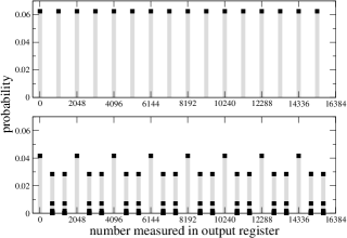
Figure 4: Distribution of measurement outcomes for factoring 119 with $x=92$ (upper) and $x=93$ (lower) which have periods $r=16$ and 24 respectively. Symbols show the probability of measuring the number on the ordinate as the outcome of the algorithm; drop lines are for clarity. The upper figure has just 16 peaks, while the lower figure shows a significant probability for measuring neighbouring numbers to the minor peaks.

This can be understood by looking at the measurement results on the larger register, from which the period $r$ is calculated. Figure 4 shows the probability of measuring each possible number $c$ in the larger register at the end of running the algorithm for two examples: factoring 119 with co-prime 92 (period $r=16$), and with co-prime 93 (period $r=24$). When the period is exactly a power of two, the fraction $c/2^{2n}$ gives the period r exactly, whereas when $r$ is not a power of two, the peak probability tries to fall between two possible numbers and thus spreads the wavefunction over several adjacent numbers. This spread corresponds to increased entanglement in the upper register. We should note that the case where $r$ is a power of two is rare for large semiprimes, so the different behaviour for $r=2^{m}$ does not help to find a factor. In fact [32], if $N$ is odd and $r=2^{m}$ for all $x$, it means that the only primes that can divide $N$ are one more than a power of $2$. There are only $5$ such odd primes known: 3, 5, 17, 257 and 65537. It is somewhat weakly conjectured that this is the complete list. But even if there are more, factoring such a number is simple: one just trial divides by numbers one more than a power of 2, more precisely, of the form $2^{2^{m}}+1$. There are approximately $\log\log N$ of them to test, so this is clearly efficient classically.

6 Discussion

First, let us summarise what we have found, since there are several steps to the deductions, necessitated by the limitations of classical computational power available to us. In this particular gate model, the first half of Shor’s algorithm, the modular exponentiation, generates approximately $\log r$ units of entropy of entanglement between the two registers [9]. Our simulations suggest that this is the only entanglement at this point, the entanglement within each register being zero. By examining the gate sequence within the IQFT we then observed that the IQFT can only generate entanglement within the upper register, or, move entanglement around between the upper register qubits. Our simulations detected both these possibilities: for $N=15$ and $N=21$ with co-prime $x=13$, the entanglement between the registers moves around the upper register qubits, while for $N=21$ and $x=2$, there is entanglement generated within the upper register during the IQFT (detected by the calculating the negativity). From examining the entropy of subsets of qubits, we deduced that the overall entanglement becomes more multipartite, because the entanglement entropy of one and two qubit subsystems decreased, while that of three to nine qubit subsystems increased. We then moved on to larger semiprimes, for which we could only calculate the one qubit subsystem entropy. Based on the pattern for $N=21$ just described, we expect this to decrease during the IQFT, corresponding to increasing multipartite entanglement, and this is what we observed, except where the period $r$ is a power of two, when it remains equal to zero.

The correlation we observe is between entanglement changes in the upper register during the IQFT, and how close the period $r$ is to a power of two. We can explain this quite easily in terms of the fraction $c/2^{2n}\simeq k/r$ that is being represented in a binary register of size $2n$. If $r$ is not a power of two, $c$ is trying to fall between two integers, and this results in a spread in the wavefunction in the final state of the quantum register, as shown in fig. 4. Extra terms in the decomposition of the final state, c.f. eq. (3), correspond to more multipartite entanglement. Now suppose we performed the IQFT in some other base than two – for example, in base three, perhaps using a quantum register made up of qutrits (three-state quantum systems) rather than qubits – the entanglement pattern would change completely. The entanglement pattern we have found is thus implementation dependent, it does not correlate with the success of the algorithm, or the number being factored. Nor is any entanglement used up during the course of the computation.

Our results support the view that entanglement is not used in a quantitative way to achieve a quantum computation faster than classical computation. While entanglement is certainly generated in significant quantities during pure state quantum computation, this is best understood as a by-product of exploiting the full Hilbert space for quantum parallelism [2, 3, 34, 33]: most of Hilbert space consists of highly entangled states [30, 35], so generation of entanglement during quantum computation is simply unavoidable.

This is to be viewed in contrast with quantum communications tasks, where maximally entangled pairs of qubits can perform a specific amount of communication, using up the entangled pairs in direct proportion to the communication achieved. We also note that entanglement is used quantitatively in many practical proposals for implementations of a quantum computer, notably [36]: this use can be identified with carrying out communications tasks to move the quantum data around in the physical qubits.

We thank Mary Beth Ruskai, Stephen Parker, Martin Plenio and Ben Travaglione for valuable discussions. VK was funded by the UK Engineering and Physical Sciences Research Council grant number GR/N2507701 (to Sept 2003) and now by a Royal Society University Research Fellowship. A Royal Society Research Grant provided additional computing facilities.

References

- [1] S. Braunstein, H.-K. Lo (Eds.), Scalable Quantum Computers: Paving the Way to Realization, Vol. 48, Fortschr. Phys., 2000.
- [2] R. Jozsa, Entanglement and quantum computation, in: S. A. Huggett, L. J. Mason, K. P. Tod, S. Tsou, N. M. J. Woodhouse (Eds.), The Geometric Universe, Geometry, and the Work of Roger Penrose, Oxford University Press, 1998, pp. 369–379.
- [3] R. Jozsa, N. Linden, On the role of entanglement in quantum computational speed-up, Proc. Roy. Soc. Lond. A Mat. 459 459 (2036) (2003) 2011–2032, quant-ph/0201143.
- [4] M. A. Nielsen, I. J. Chuang, Quantum Computation and Quantum Information, Cambridge University Press, Cambs. UK, 2000.
- [5] D. Gottesman, A theory of fault-tolerant quantum computation, Phys. Rev. A 57 (1998) 127, quant-ph/9702029.
- [6] P. W. Shor, Polynomial-time algorithms for prime factorization and discrete logarithms on a quantum computer, SIAM J. Sci Statist. Comput. 26 (1997) 1484, quant-ph/9508027.
- [7] M. Agrawal, N. Kayal, N. Saxena, Primes is in p, Annals of Mathematics 160 (2) (2004) 781–793.
- [8] A. M. Childs, R. Cleve, E. Deotto, E. Farhi, S. Gutmann, D. A. Spielman, Exponential algorithmic speedup by a quantum walk, in: Proc. 35th Annual ACM STOC, ACM, NY, 2003, pp. 59–68, quant-ph/0209131.
- [9] M. Nielsen, I. Chuang, talk at ITP Workshop (1995).
- [10] C. H. Bennett, G. Brassard, C. Crépeau, R. Jozsa, A. Peres, W. K. Wootters, Teleporting an unknown quantum state via dual classical and einstein-podolsky-rosen channels, Phys. Rev. Lett. 70 (1993) 1895–1899.
- [11] C. H. Bennett, S. J. Wiesner, Communication via one- and two-particle operators on einstein-podolsky-rosen states, Phys. Rev. Lett. 69 (20) (1992) 2881–2884.
- [12] G. Vidal, Efficient classical simulation of slightly entangled quantum computations, Phys. Rev. Lett. 91 (2003) 147902, quant-ph/0301063.
- [13] R. Orus, J. I. Latorre, Universality of entanglement and quantum computation complexity, Phys. Rev. A 69 (2004) 052308, quant-ph/0311017.
- [14] A. Ukena, A. Shimizu, Macroscopic entanglement in quantum computation, quant-ph/0505057 (2005).
- [15] Y. Shimoni, D. Shapira, O. Biham, Entangled quantum states generated by Shor’s factoring algorithm, quant-ph/0510042 (2005).
- [16] S. Parker, M. B. Plenio, Entanglement simulations of Shor’s algorithm, J. Mod. Optic 49 (8) (2001) 1325–1353, quant-ph/0102136.
- [17] V. Vedral, A. Barenco, A. Ekert, Quantum networks for elementary arithmetic operations, Phys. Rev. A 54 (1996) 147–153.
- [18] P. Gossett, Carry-save arithmetic, quant-ph/9808061 (1998).
- [19] R. V. Meter, K. M. Itoh, Fast quantum modular exponentiation, Phys. Rev. A 71 (2005) 052320, quant-ph/0408006.
- [20] C. Zalka, Fast versions of Shor’s quantum factoring algorithm, quant-ph/9806084 (1998).
- [21] S. Beauregard, Circuit for Shor’s algorithm using 2n+3 qubits, Quantum Information and Computation 3 (2) (2003) 175–185, quant-ph/0205095.
- [22] A. G. Fowler, L. C. L. Hollenberg, Scalability of Shor’s algorithm with a limited set of rotation gates, Phys. Rev. A 70 (2004) 032329, quant-ph/0306018.
- [23] D. E. Knuth, The Art of Computer Programming, Vol. 2: Seminumerical Algorithms, 2nd ed., Addison Wesley, 1981.
- [24] A. Peres, Separability criterion for density matrices, Phys. Rev. Lett. 77 (1996) 1413–1415, quant-ph/9604005.
- [25] K. Życzkowski, P. Horodecki, A. Sanpera, M. Lewenstein, On the volume of the set of mixed entangled states, Phys. Rev. A 58 (1998) 883–892.
- [26] M. Horodecki, P. Horodecki, R. Horodecki, Mixed-state entanglement and distillation: is there a “bound” entanglement in nature?, Phys. Rev. Lett. 80 (1998) 5239–5242, quant-ph/9801069.
- [27] P. Horodecki, M. Horodecki, R. Horodecki, Bound entanglement can be activated, Phys. Rev. Lett. 82 (1999) 1056–1059, quant-ph/9801069.
- [28] W. K. Wootters, Entanglement of formation of an arbitrary state of two qubits, Phys. Rev. Lett. 80 (1998) 2245–2248, quant-ph/9709029.
- [29] V. Coffman, J. Kundu, W. K. Wootters, Distributed entanglement, Phys. Rev. A 61 (2000) 052306, quant-ph/9907047.
- [30] V. M. Kendon, K. Życzkowski, W. J. Munro, Bounds on entanglement in qudit systems, Phys. Rev. A 66 (2002) 062310, quant-ph/0203037.
- [31] D. M. Greenberger, M. Horne, A. Zeilinger, Going beyond bell’s theorem, in: M. Kafatos (Ed.), Bell’s Theorem, Quantum Theory, and Conceptions of the Universe, Kluwer, 1989, pp. 73–76.
- [32] We thank Carl Pomerance and Mary Beth Ruskai for informing us about this piece of number theory (private communication), and also for the curious fact that the set of numbers (not necessarily semiprimes) for which is allowable is precisely the set of numbers for which a regular -gon is constructible with straight-edge and compass. (2005).
- [33] R. Blume-Kohout, C. M. Caves, I. H. Deutsch, Climbing mount scalable: Physical resource requirements for a scalable quantum computer, Found. Phys. 32 (11) (2002) 1641, quant-ph/0204157.
- [34] A. D. Greentree, S. G. Schirmer, F. Green, L. C. L. Hollenberg, A. R. Hamilton, R. G. Clark, Maximizing the hilbert space for a finite number of distinguishable quantum states, Phys. Rev. Lett. 92 (2004) 097901, quant-ph/0304050.
- [35] P. Hayden, D. W. Leung, A. Winter, Aspects of generic entanglement, Comm. Math. Phys. March 2006 (2006) in pressQuant-ph/0407049.
- [36] R. Raussendorf, H. J. Briegel, A one-way quantum computer, Phys. Rev. Lett. 86 (2001) 5188–5191.