The Measurement Calculus

Abstract

We propose a calculus of local equations over one-way computing patterns [RBB03], which preserves interpretations, and allows the rewriting of any pattern to a standard form where entanglement is done first, then measurements, then local corrections. We infer from this that patterns with no dependencies, or using only Pauli measurements, can only realise unitaries belonging to the Clifford group.

1 Introduction

The one-way model centres on 1-qubit measurements as the main ingredient of quantum computation [RBB03], and is believed by physicists to lend itself to easier implementations [Nie04, ND04, BR04, CAJ04]. During computations, measurements and local corrections are allowed to depend on the outcomes of previous measurements.

We first develop a notation for such classically correlated sequences of entanglements, measurements, and local corrections. Computations are organised in patterns, and we give a careful treatment of pattern composition and tensor products (parallel composition) of patterns. We show next that such pattern combinations reflect the corresponding combinations of unitary operators. An easy proof of universality, based on a family of 2-qubit patterns follows.

So far, this constitutes mostly a work of clarification of what was already known from the series of papers introducing and investigating the properties of the one-way model [RBB03]. However, we work here with an extended notion of pattern, where inputs and outputs may overlap in any way one wants them to, and this obtains more efficient - in the sense of fewer qubits - implementations of unitaries. Specifically, our generating set consists of two simple patterns, each one using only 2 qubits. From it we obtain a 3 qubits realisation of the $R_{z}$ rotations and a 14 qubit implementation for the controlled-$U$ family: a very significant reduction over the known implementations.

However, the main point of this paper is to introduce alongside our notation, a calculus of local equations over patterns that exploits the fact that 1-qubit $xy$-measurements are closed under conjugation by Pauli operators. We show that this calculus is sound in that it preserves the patterns interpretations. Most importantly, we derive from it a simple algorithm by which any general pattern can be put into a standard form where entanglement is done first, then measurements, then corrections.

The consequences of the existence of such a procedure are far-reaching. First, since entangling comes first, one can prepare the entire entangled state needed during the computation right at the start: one never has to do “on the fly” entanglements. Second, since local corrections come last, only the output qubits will ever need corrections. Third, the rewriting of a pattern to standard form reveals parallelism in the pattern computation. In a general pattern, one is forced to compute sequentially and obey strictly the command sequence, whereas after standardisation, the dependency structure is relaxed, resulting in low depth complexity. Last, the existence of a standard form for any pattern also has interesting corollaries beyond implementation and complexity matters, as it follows from it that patterns using no dependencies, or using only the restricted class of Pauli measurements, can only realise a unitary belonging to the Clifford group.

Acknowledgements: Elham Kashefi wishes to express her gratitude to Quentin for letting her collaborate with his father, Vincent Danos, during their stay in Canada. Prakash Panangaden wishes to express his gratitude to EPSRC for supporting his stay in Oxford where this collaboration began.

2 Computation Patterns

We first develop a notation for 1-qubit measurement based computations. The basic commands one can use are:

• 1-qubit measurements ${M}_{i}^{\alpha}$

• 2-qubit entanglement operators $E_{ij}$

• and 1-qubit Pauli corrections $X_{i}$, $Z_{i}$

The indices $i$, $j$ represent the qubits on which each of these operations apply, and $\alpha$ is a parameter in $[0,2\pi]$. Sequences of such commands, together with two distinguished —possibly overlapping— sets of qubits corresponding to inputs and outputs, will be called measurement patterns, or simply patterns. These patterns can be combined by composition and tensor product.

Importantly corrections and measurements are allowed to depend on previous measurement outcomes. We shall prove later that patterns without those classical dependencies can only realise unitaries that are in the Clifford group. Thus dependencies are crucial if one wants to define a universal computing model; that is to say a model where all finite-dimensional unitaries can be realised, and it is also crucial to develop a notation that will handle these dependencies gracefully.

2.1 Commands

The entanglement commands are defined as $E_{ij}:=\mathop{\wedge}\hskip-1.72218ptZ_{ij}$, while the correction commands are the Pauli operators $X_{i}$ and $Z_{i}$.

A 1-qubit measurement command, written ${M}_{i}^{\alpha}$, is given by a pair of complement orthogonal projections, on:

$${|}\hskip-0.43057pt+_{\alpha}\rangle := \frac{1}{\sqrt{2}}({|}0\rangle+e^{i\alpha}{|}1\rangle)$$ (1)

$${|}\hskip-0.43057pt-_{\alpha}\rangle := \frac{1}{\sqrt{2}}({|}0\rangle-e^{i\alpha}{|}1\rangle)$$ (2)

It is easily seen that ${|}\hskip-0.43057pt+_{\alpha}\rangle$, ${|}\hskip-0.43057pt-_{\alpha}\rangle$ form an orthonormal basis in ${\mathbb{C}}^{2}$, so they indeed define a 1-qubit measurement (of rank $2^{n-1}$, if $n$ is the number of qubits in the ambient computing space). Measurements here will always be understood as destructive measurements, that is to say the concerned qubit is consumed in the measurement operation.

The outcome of a measurement done at qubit $i$ will be denoted by $s_{i}\in{\mathbb{Z}}_{2}$. Since one only deals with patterns where qubits are measured at most once (see condition (D1) below), this is unambiguous. We take the convention that $s_{i}=0$ if under the corresponding measurement the state collapses to ${|}\hskip-0.43057pt+_{\alpha}\rangle$, and $s_{i}=1$ if to ${|}\hskip-0.43057pt-_{\alpha}\rangle$.

Outcomes can be summed together resulting in expressions of the form $s=\sum_{i\in I}s_{i}$ which we call signals, and where the summation is understood as being done is ${\mathbb{Z}}_{2}$. We define the domain of a signal as the set of qubits it depends on.

Dependent corrections will be written $X_{i}^{s}$ and $Z_{i}^{s}$ with $s$ a signal. Their meaning is that $X_{i}^{0}=Z_{i}^{0}=I$ (no correction is applied), while $X_{i}^{1}=X_{i}$ and $Z_{i}^{1}=Z_{i}$.

Dependent measurements will be written ${}^{t}[{M}_{i}^{\alpha}]^{s}$, where $s$ and $t$ are signals. Their meaning is as follows:

$${}^{t}[{M}_{i}^{\alpha}]^{s} := {M}_{i}^{(-1)^{s}\alpha+t\pi}$$ (3)

As a result, before applying a measurement, one has to know first all the measurements outcomes occurring in the signals $s$, $t$, then one has to compute the parity of $s$ and $t$, and maybe modify $\alpha$ to one of $-\alpha$, $\alpha+\pi$ and $-\alpha+\pi$. One can easily compute that:

$$X_{i}{M}_{i}^{{\alpha}}X_{i} = {M}_{i}^{{-\alpha}}$$ (4)

$$Z_{i}{M}_{i}^{{\alpha}}Z_{i} = {M}_{i}^{{\alpha+\pi}}$$ (5)

so that the actions correspond to conjugations of measurements under $X$ and $Z$. We will refer to them as the $X$ and $Z$-actions. Note that these two actions are commuting, since $-\alpha+\pi=-\alpha-\pi$ up to $2\pi$, and hence the order in which one applies them doesn’t matter. Should one use other local corrections, then one would have here instead the corresponding actions on measurement angles. As we will see later, relations (4) and (5) are key to the propagation of dependent corrections, and to obtaining patterns in the standard entanglement, measurement, correction form. Since measurements considered here are destructive ones, the equations simplify to ${M}_{i}^{{\alpha}}X_{i}={M}_{i}^{{-\alpha}}$, and ${M}_{i}^{{\alpha}}Z_{i}={M}_{i}^{{\alpha+\pi}}$.

Another point worth noticing is that the domain of the signals of a dependent command, be it a measurement or a correction, represents the set of measurements which one has to do before one can determine the actual value of the command.

Finally we note that we could work with general 1-qubit measurements, instead of the class defined above, sometimes called $xy$-measurements. All the developments would carry through nicely, but we have not found so far any compelling reason for this additional generality.

2.2 Patterns

Definition 1

Patterns consists of three finite sets $V$, $I$, $O$, together with two injective maps $\iota:I\rightarrow V$ and $o:O\rightarrow V$ and a finite sequence of commands $A_{n}\ldots A_{1}$ applying to qubits in $V$.

The set $V$ is called the pattern computation space, and we write $\mathfrak{H}_{V}$ for the associated quantum state space $\otimes_{i\in V}{\mathbb{C}}^{2}$. To ease notation, we will forget altogether about the maps $\iota$ and $o$, and write simply $I$, $O$ instead of $\iota(I)$ and $o(O)$. Note however, that these maps are useful to define classical manipulations of the quantum states, such as permutations of the qubits. The sets $I$, $O$ will be called respectively the pattern inputs and outputs, and we will write $\mathfrak{H}_{I}$, and $\mathfrak{H}_{O}$ for the associated quantum state spaces. The sequence $A_{n}\ldots A_{1}$ will be called the pattern command sequence.

To run a pattern, one prepares the input qubits in some input state $\psi\in\mathfrak{H}_{I}$, while the non-input qubits are all set in the ${|}+\rangle$ state, then the commands are executed in sequence, and finally the result of the pattern computation is some $\phi\in\mathfrak{H}_{O}$. There might be qubits in the pattern, which are neither inputs nor outputs qubits, and are used as auxiliary qubits during the computation. Usually one tries to use as few of them as possible, since these participate to the space complexity of the computation.

Note that one does not require inputs and outputs to be disjoint subsets of $V$. This seemingly innocuous additional flexibility is actually quite useful to give parsimonious implementations of unitaries [DKP04]. While the restriction to disjoint inputs and outputs is unnecessary, it has been discussed whether more constrained patterns might be easier to realise physically. Recent work [HEB04, BR04, CAJ04] however, seems to indicate they are not.

Here is an example of a pattern implementing the Hadamard operator $H$:

$$\begin{array}[c]{lllllllllllllll}\mathfrak{H}&:=&(\{1,2\},\{1\},\{2\},X_{2}^{s_{1}}{M}_{1}^{0}E_{12})\end{array}$$

What is this pattern doing ? The first qubit is prepared in some input state $\psi$, and the second in state ${|}+\rangle$, then these are entangled to obtain $\mathop{\wedge}\hskip-1.72218ptZ_{12}(\psi_{1}\otimes{|}+\rangle_{2})$. Once this is done, the first qubit is measured in the ${|}+\rangle$, ${|}-\rangle$ basis. Finally an $X$ correction is applied on the output qubit, depending on the outcome of the measurement. We will do this calculation in detail later.

2.3 Pattern combination

We are interested now in how one can combine patterns into bigger ones.

The first way to combine patterns is by composing them. Two patterns $\mathfrak{P}_{1}$ and $\mathfrak{P}_{2}$ may be composed if $V_{1}\cap V_{2}=O_{1}=I_{2}$. Note that provided that $\mathfrak{P}_{1}$ has as many outputs as $\mathfrak{P}_{2}$ has inputs, by renaming the pattern qubits, one can always make them composable.

Definition 2

The composite pattern $\mathfrak{P}_{2}\mathfrak{P}_{1}$ is defined as:
— $V:=V_{1}\cup V_{2}$, $I=I_{1}$, $O=O_{2}$,
— commands are concatenated.

The other way of combining patterns is to tensor them. Two patterns $\mathfrak{P}_{1}$ and $\mathfrak{P}_{2}$ may be tensored if $V_{1}\cap V_{2}=\varnothing$. Again one can always meet this condition by renaming qubits in a way that these sets are made disjoint.

Definition 3

The tensor pattern $\mathfrak{P}_{2}\otimes\mathfrak{P}_{1}$ is defined as:
— $V=V_{1}\cup V_{2}$, $I=I_{1}\cup I_{2}$, and $O=O_{1}\cup O_{2}$,
— commands are concatenated.

Note that all unions above are disjoint. Note also that, in opposition to the composition case, commands from distinct patterns freely commute, since they apply to disjoint qubits and are independent of each other, so when we say that commands have to be concatenated, this is only for definiteness.

2.4 Pattern conditions

One might want to subject patterns to various conditions:

(D0)

no command depends an outcome not yet measured;

(D1)

no command acts on a qubit already measured;

(D2)

a qubit $i$ is measured if and only if $i$ is not an output;

(EMC)

commands occur $E$s first, then $M$s, then $C$s.

The reader might want to check that our example $\mathfrak{H}$ satisfies all of the above. It is routine to verify that these conditions are preserved under composition and tensor. Conditions (D0) and (D1) ensure that a pattern can always be run meaningfully. Indeed if (D0) fails, then at some point of the computation, one will want to execute a command which depends on outcomes that are not known yet. Likewise, if (D1) fails, one will try to apply a command on a qubit that has been consumed by a measurement (recall that we use destructive measurements). Condition (D2) is there to make sure that at the end of running the pattern, the state will belong to the output space $\mathfrak{H}_{O}$, i.e., that all non-output qubits, and only them, will have been consumed by a measurement when the computation ends.

Starting now we will assume that all patterns satisfy the definiteness conditions (D0), (D1) and (D2), and will designate by (D) the conjunction of these three conditions.

Condition (EMC) is of a completely different nature. Patterns not respecting it will be called wild.

Later on, we will introduce the measurement calculus and show a simple rewriting procedure turning any given wild pattern into an equivalent one which is in (EMC) form. We call this procedure standardisation, and also say that a pattern meeting the (EMC) condition is standard.

Before turning to this matter, we need a clean definition of what it means for a pattern to implement or to realise a unitary operator, together with a proof that the way one can combine patterns is reflected in their interpretations. This is key to our proof of universality.

3 Computing a pattern

Besides quantum states which are vectors in some $\mathfrak{H}_{V}$, one needs a classical state recording the outcomes of the successive measurements one does in a pattern. So it is natural to define the computation state space as:

$$\begin{array}[c]{lllllllllllllll}\mathcal{S}&:=&\bigcup_{V,W}\mathfrak{H}_{V}\times{\mathbb{Z}}_{2}^{W}\end{array}$$

where $V$, $W$ range over finite sets. In other words a computation state is a pair $q$, $\Gamma$, where $q$ is a quantum state and $\Gamma$ is a map from some $W$ to the outcome space ${\mathbb{Z}}_{2}$. We call this classical component $\Gamma$ an outcome map and denote by $\varnothing$ the unique map in ${\mathbb{Z}}_{2}^{\varnothing}$.

3.1 Commands as actions

We need a few notations. For any signal $s$ and classical state $\Gamma\in{\mathbb{Z}}_{2}^{W}$, such that the domain of $s$ is included in $W$, we take $s_{\Gamma}$ to be the value of $s$ given by the outcome map $\Gamma$. That is to say, if $s=\sum_{I}s_{i}$, then $s_{\Gamma}:=\sum_{I}\Gamma(i)$ where the sum is taken in ${\mathbb{Z}}_{2}$. Also if $\Gamma\in{\mathbb{Z}}_{2}^{W}$, and $x\in{\mathbb{Z}}_{2}$, we define:

$$\begin{array}[c]{lllllllllllllll}\Gamma[x/i](i)=x,\,\Gamma[x/i](j)=\Gamma(j)\hbox{ for }j\neq i\end{array}$$

which is a map in ${\mathbb{Z}}_{2}^{W\cup\{i\}}$.

We may now see each of our commands as acting on $\mathcal{S}$.

$$\begin{array}[c]{lllllllllllllll}q,\Gamma&\stackrel{{\scriptstyle E_{ij}}}{{\longrightarrow}}&\mathop{\wedge}\hskip-1.72218ptZ_{ij}q,\Gamma\\ q,\Gamma&\stackrel{{\scriptstyle X_{i}^{s}}}{{\longrightarrow}}&X_{i}^{s_{\Gamma}}q,\Gamma\\ q,\Gamma&\stackrel{{\scriptstyle Z_{i}^{s}}}{{\longrightarrow}}&Z_{i}^{s_{\Gamma}}q,\Gamma\\ q,\Gamma&\stackrel{{\scriptstyle{}^{t}[{M}_{i}^{\alpha}]^{s}}}{{\longrightarrow}}&{\langle\hskip-0.43057pt+_{\alpha_{\Gamma}}{|}}_{i}q,\Gamma[0/i]\\ q,\Gamma&\stackrel{{\scriptstyle{}^{t}[{M}_{i}^{\alpha}]^{s}}}{{\longrightarrow}}&{\langle\hskip-0.43057pt-_{\alpha_{\Gamma}}{|}}_{i}q,\Gamma[1/i]\end{array}$$

where $\alpha_{\Gamma}=(-1)^{s_{\Gamma}}\alpha+t_{\Gamma}\pi$ following equation (3), and $\langle\psi{|}_{i}$ is the linear form associated to $\psi$ applied at qubit $i$. Suppose $q\in\mathfrak{H}_{V}$, for the above relations to be defined, one needs the indices $i$, $j$ on which the various command apply to be in $V$. One also needs $\Gamma$ to contain the domains of $s$ and $t$, so that $s_{\Gamma}$ and $t_{\Gamma}$ are well-defined. This will always be the case during the run of a pattern because of condition (D).

All commands except measurements are deterministic and only modify the quantum part of the state. The measurements actions on $\mathcal{S}$ are not deterministic, so that these are actually binary relations on $\mathcal{S}$, and modify both the quantum and classical parts of the state. The usual convention has it that when one does a measurement the resulting state is renormalised, but we don’t adhere to it here, the reason being that this way, the probability of reaching a given state can be read off its norm, and the overall treatment is simpler.

We introduce an additional command called shifting:

$$\begin{array}[c]{lllllllllllllll}q,\Gamma&\stackrel{{\scriptstyle S_{i}^{s}}}{{\longrightarrow}}&q,\Gamma[\Gamma(i)+s_{\Gamma}/i]\end{array}$$

It consists in shifting the measurement outcome at $i$ by the amount $s_{\Gamma}$. Note that the $Z$-action leaves measurements globally invariant, in the sense that ${|}\hskip-0.43057pt+_{\alpha+\pi}\rangle,{|}\hskip-0.43057pt-_{\alpha+\pi}\rangle={|}\hskip-0.43057pt-_{\alpha}\rangle,{|}\hskip-0.43057pt+_{\alpha}\rangle$. Thus changing $\alpha$ to $\alpha+\pi$ amounts to swap the outcomes of the measurements, and one has:

$${}^{t}[{M}_{i}^{\alpha}]^{s} = S_{i}^{t}[{M}_{i}^{\alpha}]^{s}$$ (6)

and shifting allows to split the $t$ action of a measurement, resulting sometimes in convenient optimisations of standard forms.

3.2 Computation branches

Let $\mathfrak{P}$ be a pattern with computation space $V$, inputs $I$, outputs $O$ and command sequence $A_{n}\ldots A_{1}$. A complete pattern computation starts with some input state $q$ in $\mathfrak{H}_{I}$, together with the empty outcome map $\varnothing$. The input state $q$ is then tensored with as many ${|}+\rangle$s as there are non-inputs in $V$, so as to obtain a state in the full space $\mathfrak{H}_{V}$. Then commands in $\mathfrak{P}$ are applied in sequence. We can summarise the situation as follows:

$$\begin{array}[c]{lllllllllllllll}\lx@xy@svg{\hbox{\raise 0.0pt\hbox{\kern 18.54501pt\hbox{\ignorespaces\immediate\immediate\immediate{\ignorespaces{\immediate}{\immediate}{\immediate}{\immediate}{\immediate}{\immediate}{\immediate}{\immediate}{\immediate}{\immediate}{\immediate}{\immediate}{\immediate}{\immediate}{\immediate}{\immediate}{\immediate}{\immediate}{\immediate}{\immediate}{\immediate}{\immediate}{\immediate}{\immediate}{\immediate}{\immediate}{\immediate}{\immediate}{\immediate}{\immediate}{\immediate}{\immediate}{\immediate}{\immediate}{\immediate}{\immediate}{\immediate}{\immediate}{\immediate}{\immediate}{\immediate}{\immediate}{\immediate}{\immediate}{\immediate}{\immediate}{\immediate}{\immediate}{\immediate}{\immediate}\hbox{\vtop{{\immediate}\kern 0.0pt\offinterlineskip\halign{\entry@#!@&&\entry@@#!@\cr{\immediate}{\immediate}{\immediate}&{\immediate}{\immediate}{\immediate}&{\immediate}{\immediate}{\immediate}\\{\immediate}{\immediate}{\immediate}&{\immediate}{\immediate}{\immediate}&{\immediate}{\immediate}{\immediate}\crcr}{\immediate}}}{\immediate}{\immediate}\ignorespaces{\immediate}{\immediate}\ignorespaces}\immediate\immediate\ignorespaces\ignorespaces\ignorespaces{\hbox{\kern-10.20055pt\raise 0.0pt\hbox{\hbox{\kern 0.0pt\raise 0.0pt\hbox{\hbox{\kern 5.0pt\raise 0.0pt\hbox{$\textstyle{{}\mathfrak{H}_{I}\ignorespaces\ignorespaces\ignorespaces\ignorespaces\ignorespaces\ignorespaces\ignorespaces\ignorespaces}$}}}}}}}\ignorespaces\ignorespaces\ignorespaces\ignorespaces{}{\hbox{\lx@xy@droprule}}\ignorespaces{\hbox{\kern 0.0pt\raise-25.86333pt\hbox{\hbox{\kern 0.0pt\raise 0.0pt\hbox{\lx@xy@tip{1}\lx@xy@tip{-1}}}}}}{\hbox{\lx@xy@droprule}}{\hbox{\lx@xy@droprule}}\ignorespaces\ignorespaces\ignorespaces{}\ignorespaces\ignorespaces{\hbox{\lx@xy@drawline@}}\ignorespaces{\hbox{\kern 145.58952pt\raise 0.0pt\hbox{\hbox{\kern 0.0pt\raise 0.0pt\hbox{\lx@xy@tip{1}\lx@xy@tip{-1}}}}}}\ignorespaces\ignorespaces{\hbox{\lx@xy@drawline@}}\ignorespaces{\hbox{\lx@xy@drawline@}}{\hbox{\kern 72.89503pt\raise 0.0pt\hbox{\hbox{\kern 0.0pt\raise 0.0pt\hbox{\hbox{\kern 5.0pt\raise 0.0pt\hbox{$\textstyle{}$}}}}}}}{\hbox{\kern 145.58952pt\raise 0.0pt\hbox{\hbox{\kern 0.0pt\raise 0.0pt\hbox{\hbox{\kern 5.0pt\raise 0.0pt\hbox{$\textstyle{{}\mathfrak{H}_{O}}$}}}}}}}{\hbox{\kern-18.54501pt\raise-39.79665pt\hbox{\hbox{\kern 0.0pt\raise 0.0pt\hbox{\hbox{\kern 5.0pt\raise 0.0pt\hbox{$\textstyle{{}\mathfrak{H}_{I}\times{\mathbb{Z}}_{2}^{\varnothing}\ignorespaces\ignorespaces\ignorespaces\ignorespaces}$}}}}}}}\ignorespaces\ignorespaces\ignorespaces\ignorespaces{}{\hbox{\lx@xy@droprule}}\ignorespaces\ignorespaces\ignorespaces{\hbox{\kern 29.11966pt\raise-34.60915pt\hbox{{}\hbox{\kern 0.0pt\raise 0.0pt\hbox{\hbox{\kern 3.0pt\hbox{\hbox{\kern 0.0pt\raise-0.8264pt\hbox{$\scriptstyle{prep}$}}}\kern 3.0pt}}}}}}\ignorespaces{\hbox{\kern 58.54501pt\raise-39.79665pt\hbox{\hbox{\kern 0.0pt\raise 0.0pt\hbox{\lx@xy@tip{1}\lx@xy@tip{-1}}}}}}{\hbox{\lx@xy@droprule}}{\hbox{\lx@xy@droprule}}{\hbox{\kern 58.54501pt\raise-39.79665pt\hbox{\hbox{\kern 0.0pt\raise 0.0pt\hbox{\hbox{\kern 5.0pt\raise 0.0pt\hbox{$\textstyle{{}\mathfrak{H}_{V}\times{\mathbb{Z}}_{2}^{\varnothing}\ignorespaces\ignorespaces\ignorespaces\ignorespaces}$}}}}}}}\ignorespaces\ignorespaces\ignorespaces\ignorespaces{}{\hbox{\lx@xy@droprule}}\ignorespaces\ignorespaces\ignorespaces{\hbox{\kern 100.64857pt\raise-33.64665pt\hbox{{}\hbox{\kern 0.0pt\raise 0.0pt\hbox{\hbox{\kern 3.0pt\hbox{\hbox{\kern 0.0pt\raise-1.75pt\hbox{$\scriptstyle{A_{1}\ldots A_{n}\quad}$}}}\kern 3.0pt}}}}}}\ignorespaces{\hbox{\kern 137.24506pt\raise-39.79665pt\hbox{\hbox{\kern 0.0pt\raise 0.0pt\hbox{\lx@xy@tip{1}\lx@xy@tip{-1}}}}}}{\hbox{\lx@xy@droprule}}{\hbox{\lx@xy@droprule}}{\hbox{\kern 137.24506pt\raise-39.79665pt\hbox{\hbox{\kern 0.0pt\raise 0.0pt\hbox{\hbox{\kern 5.0pt\raise 0.0pt\hbox{$\textstyle{{}\mathfrak{H}_{O}\times{\mathbb{Z}}_{2}^{V\setminus O}\ignorespaces\ignorespaces\ignorespaces\ignorespaces}$}}}}}}}\ignorespaces\ignorespaces\ignorespaces\ignorespaces{}{\hbox{\lx@xy@droprule}}\ignorespaces{\hbox{\kern 156.55307pt\raise-6.91333pt\hbox{\hbox{\kern 0.0pt\raise 0.0pt\hbox{\lx@xy@tip{1}\lx@xy@tip{-1}}}}}}{\hbox{\lx@xy@droprule}}{\hbox{\lx@xy@droprule}}}}}}\ignorespaces\end{array} \textstyle{{}\mathfrak{H}_{I}\ignorespaces\ignorespaces\ignorespaces\ignorespaces\ignorespaces\ignorespaces\ignorespaces\ignorespaces} \textstyle{{}\mathfrak{H}_{O}} \textstyle{{}\mathfrak{H}_{I}\times{\mathbb{Z}}_{2}^{\varnothing}\ignorespaces\ignorespaces\ignorespaces\ignorespaces} \scriptstyle{prep} \textstyle{{}\mathfrak{H}_{V}\times{\mathbb{Z}}_{2}^{\varnothing}\ignorespaces\ignorespaces\ignorespaces\ignorespaces} \scriptstyle{A_{1}\ldots A_{n}\quad} \textstyle{{}\mathfrak{H}_{O}\times{\mathbb{Z}}_{2}^{V\setminus O}\ignorespaces\ignorespaces\ignorespaces\ignorespaces} \textstyle{{}\mathfrak{H}_{I}\ignorespaces\ignorespaces\ignorespaces\ignorespaces\ignorespaces\ignorespaces\ignorespaces\ignorespaces} \textstyle{{}\mathfrak{H}_{O}} \textstyle{{}\mathfrak{H}_{I}\times{\mathbb{Z}}_{2}^{\varnothing}\ignorespaces\ignorespaces\ignorespaces\ignorespaces} \scriptstyle{prep} \textstyle{{}\mathfrak{H}_{V}\times{\mathbb{Z}}_{2}^{\varnothing}\ignorespaces\ignorespaces\ignorespaces\ignorespaces} \scriptstyle{A_{1}\ldots A_{n}\quad} \textstyle{{}\mathfrak{H}_{O}\times{\mathbb{Z}}_{2}^{V\setminus O}\ignorespaces\ignorespaces\ignorespaces\ignorespaces}$$

To make this precise, say there is a $\mathfrak{P}$-branch from $q\in\mathfrak{H}_{I}$ to $q^{\prime}\in\mathfrak{H}_{O}$, written $q\rightarrow_{\mathfrak{P}}q^{\prime}$, if there is a sequence $(q_{i},\Gamma_{i})$ with $1\leq i\leq n+1$, such that:

$$\begin{array}[c]{lllllllllllllll}q\otimes{|}\hskip-1.72218pt+\ldots+\rangle,\varnothing=q_{1},\Gamma_{1}\\ q^{\prime}=q_{n+1}\neq 0\\ \hbox{and for all }i\leq n:q_{i},\Gamma_{i}\stackrel{{\scriptstyle A_{i}}}{{\longrightarrow}}q_{i+1},\Gamma_{i+1}\end{array}$$

thus $\rightarrow_{\mathfrak{P}}$ is a binary relation on $\mathfrak{H}_{I}\times\mathfrak{H}_{O}$. That it is a relation and not a map reflects the fact that measurements a priori introduce non determinism in the evolution of the quantum states.

Specifically, if $k$ is the number of measurements in $\mathfrak{P}$ (or equivalently the number of non-outputs qubits), there are at most $2^{k}$ branches in any given computation, and therefore a given $q\in\mathfrak{H}_{I}$ is in relation with at most $2^{k}$ distinct $q^{\prime}\in\mathfrak{H}_{O}$. The probability of a branch is defined to be $\|q^{\prime}\|^{2}/\|q\|^{2}$ ($q$ being always assumed to be non zero). Indeed one has:

$$\sum_{\{q^{\prime}\mid q\rightarrow_{\mathfrak{P}}q^{\prime}\}}\|q^{\prime}\|^{2} = \|q\|^{2}$$ (7)

since any action is either a unitary, thus a norm-preserving action, or a measurement which introduces a branching, and then if $q$ projects to $q_{0}$ and $q_{1}$, under some ${M}_{i}^{\alpha}$, $\|q\|^{2}=\|q_{0}\|^{2}+\|q_{1}\|^{2}$, so that the relation above is always preserved.

Definition 4

One says the pattern $\mathfrak{P}$ is deterministic if for all $q\in\mathfrak{H}_{I}$, $q^{\prime}$ and $q^{\prime\prime}\in\mathfrak{H}_{O}$, whenever $q\rightarrow_{\mathfrak{P}}q^{\prime}$ and $q\rightarrow_{\mathfrak{P}}q^{\prime\prime}$, then $q^{\prime}$ and $q^{\prime\prime}$ only differ up to a scalar.

Note that even when $\mathfrak{P}$ is deterministic, all branches might not be equally likely. When $\mathfrak{P}$ is deterministic, one defines a norm-preserving map $U_{\mathfrak{P}}$ from $\mathfrak{H}_{I}$ to $\mathfrak{H}_{O}$ by:

$$U_{\mathfrak{P}}(q) := \frac{\|q\|}{\|q^{\prime}\|}q^{\prime}$$ (8)

Note that when $q\rightarrow_{\mathfrak{P}}q^{\prime}$, $q^{\prime}\neq 0$, so that the definition above always make sense. Note also that because $\mathfrak{P}$ is deterministic, this map depends on the choice of $q^{\prime}$ only up to a global phase. One can further comment that since we took the convention not to renormalise measurement results, we have to do here a global renormalisation to define the pattern interpretation.

One says that a deterministic pattern $\mathfrak{P}$ realises or implements $U_{\mathfrak{P}}$, or equivalently that $U_{\mathfrak{P}}$ is the interpretation of $\mathfrak{P}$.

This map $U_{\mathfrak{P}}$ must actually be a unitary embedding, since all quantum definable deterministic transformations are unitaries. If a precise argument is needed here, one can rephrase all the definitions given so far in the language of density operators and completely-positive maps (cp-maps). Then a deterministic pattern will implement a cp-map preserving pure density operators. From the Kraus representation theorem for cp-maps, it is easy to see that such cp-maps are liftings of unitary embeddings.

3.3 Short examples

First we give a quick example of a deterministic pattern that has branches with different probabilities. The state space is $\{1,2\}$, with $I=O=\{1\}$, while the command sequence is ${M}_{2}^{\alpha}$. Therefore, starting with input $q$, one gets two branches:

$$\begin{array}[c]{lllllllllllllll}q\otimes{|}+\rangle,\varnothing&\stackrel{{\scriptstyle{M}_{2}^{\alpha}}}{{\longrightarrow}}&\left\{\begin{array}[]{l}\frac{1}{2}(1+e^{{-i}\alpha})q,\varnothing[0/2]\\ \\ \frac{1}{2}(1-e^{{-i}\alpha})q,\varnothing[1/2]\end{array}\right.\end{array}$$

Thus this pattern is indeed deterministic, and implements the identity up to a global phase, and yet the two branches have respective probabilities $(1+\cos\alpha)/2$ and $(1-\cos\alpha)/2$, which are not equal in general.

Next, we return to the pattern $\mathfrak{H}$ which we already took as an example. Let us consider for a start the pattern with same space $\{1,2\}$, same inputs and outputs $I=\{1\}$, $O=\{2\}$, and shorter command sequence ${M}_{1}^{0}E_{12}$. Starting with input $q=(a{|}0\rangle+b{|}1\rangle){|}+\rangle$, one has two computation branches, branching at ${M}_{1}^{0}$:

$$\begin{array}[c]{lllllllllllllll}(a{|}0\rangle+b{|}1\rangle){|}+\rangle,\varnothing&\stackrel{{\scriptstyle E_{12}}}{{\longrightarrow}}&\frac{1}{\sqrt{2}}(a{|}00\rangle+a{|}01\rangle+b{|}10\rangle-b{|}11\rangle),\varnothing\\ \\ &\stackrel{{\scriptstyle{M}_{1}^{0}}}{{\longrightarrow}}&\left\{\begin{array}[]{l}\frac{1}{2}((a+b){|}0\rangle+(a-b){|}1\rangle),\varnothing[0/0]\\ \\ \frac{1}{2}((a-b){|}0\rangle+(a+b){|}1\rangle),\varnothing[1/0]\end{array}\right.\end{array}$$

and since $\|a+b\|^{2}+\|a-b\|^{2}=2(\|a\|^{2}+\|b\|^{2})$, both transitions happen with equal probabilities $\frac{1}{2}$. Both branches end up with different outputs, so the pattern is not deterministic. However, if one applies the local correction $X_{2}$ on either of the branches ends, both outputs will be made to coincide. Let us choose to let the correction bear on the second branch, obtaining the example $\mathfrak{H}$ which we defined already. We have just proved $H=U_{\mathfrak{H}}$, that is to say $\mathfrak{H}$ realises the Hadamard operator.

With our definitions in place, we first infer that pattern combinations correspond to combinations of their interpretations. From this an easy structured argument - that uses surprisingly simple patterns - for universality will follow.

3.4 Composing, Tensoring and Interpretation

Recall that two patterns $\mathfrak{P}_{1}$, $\mathfrak{P}_{2}$ may be combined by composition provided $\mathfrak{P}_{1}$ have as many outputs as $\mathfrak{P}_{2}$ has inputs. Suppose this is the case, and suppose further that $\mathfrak{P}_{1}$ and $\mathfrak{P}_{2}$ respectively realise some unitaries $U_{1}$ and $U_{2}$, then the composite pattern $\mathfrak{P}_{2}\mathfrak{P}_{1}$ realises $U_{2}U_{1}$.

Indeed, the two diagrams representing branches in $\mathfrak{P}_{1}$ and $\mathfrak{P}_{2}$:

$$\begin{array}[c]{lllllllllllllll}\lx@xy@svg{\hbox{\raise 0.0pt\hbox{\kern 14.47603pt\hbox{\ignorespaces\immediate\immediate\immediate{\ignorespaces{\immediate}{\immediate}{\immediate}{\immediate}{\immediate}{\immediate}{\immediate}{\immediate}{\immediate}{\immediate}{\immediate}{\immediate}{\immediate}{\immediate}{\immediate}{\immediate}{\immediate}{\immediate}{\immediate}{\immediate}{\immediate}{\immediate}{\immediate}{\immediate}{\immediate}{\immediate}{\immediate}{\immediate}{\immediate}{\immediate}{\immediate}{\immediate}{\immediate}{\immediate}{\immediate}{\immediate}{\immediate}{\immediate}{\immediate}{\immediate}{\immediate}{\immediate}{\immediate}{\immediate}{\immediate}{\immediate}{\immediate}{\immediate}{\immediate}{\immediate}{\immediate}{\immediate}{\immediate}{\immediate}{\immediate}{\immediate}{\immediate}{\immediate}{\immediate}{\immediate}{\immediate}{\immediate}{\immediate}{\immediate}{\immediate}{\immediate}{\immediate}{\immediate}{\immediate}{\immediate}{\immediate}{\immediate}{\immediate}{\immediate}{\immediate}{\immediate}{\immediate}{\immediate}{\immediate}{\immediate}{\immediate}{\immediate}{\immediate}{\immediate}{\immediate}{\immediate}\hbox{\vtop{{\immediate}\kern 0.0pt\offinterlineskip\halign{\entry@#!@&&\entry@@#!@\cr{\immediate}{\immediate}{\immediate}&{\immediate}{\immediate}{\immediate}&{\immediate}{\immediate}{\immediate}&{\immediate}{\immediate}{\immediate}&{\immediate}{\immediate}{\immediate}&{\immediate}{\immediate}{\immediate}\\{\immediate}{\immediate}{\immediate}&{\immediate}{\immediate}{\immediate}&{\immediate}{\immediate}{\immediate}&{\immediate}{\immediate}{\immediate}&{\immediate}{\immediate}{\immediate}&{\immediate}{\immediate}{\immediate}\crcr}{\immediate}}}{\immediate}{\immediate}\ignorespaces{\immediate}{\immediate}\ignorespaces}\immediate\immediate\ignorespaces\ignorespaces\ignorespaces{\hbox{\kern-7.80045pt\raise 0.0pt\hbox{\hbox{\kern 0.0pt\raise 0.0pt\hbox{\hbox{\kern 3.0pt\raise 0.0pt\hbox{$\textstyle{{}\mathfrak{H}_{I_{1}}\ignorespaces\ignorespaces\ignorespaces\ignorespaces\ignorespaces\ignorespaces\ignorespaces\ignorespaces}$}}}}}}}\ignorespaces\ignorespaces\ignorespaces\ignorespaces{}{\hbox{\lx@xy@droprule}}\ignorespaces{\hbox{\kern 0.0pt\raise-24.51555pt\hbox{\hbox{\kern 0.0pt\raise 0.0pt\hbox{\lx@xy@tip{1}\lx@xy@tip{-1}}}}}}{\hbox{\lx@xy@droprule}}{\hbox{\lx@xy@droprule}}\ignorespaces\ignorespaces\ignorespaces{}\ignorespaces\ignorespaces{\hbox{\lx@xy@drawline@}}\ignorespaces{\hbox{\kern 65.39166pt\raise 0.0pt\hbox{\hbox{\kern 0.0pt\raise 0.0pt\hbox{\lx@xy@tip{1}\lx@xy@tip{-1}}}}}}\ignorespaces\ignorespaces{\hbox{\lx@xy@drawline@}}\ignorespaces{\hbox{\lx@xy@drawline@}}{\hbox{\kern 33.59605pt\raise 0.0pt\hbox{\hbox{\kern 0.0pt\raise 0.0pt\hbox{\hbox{\kern 3.0pt\raise 0.0pt\hbox{$\textstyle{}$}}}}}}}{\hbox{\kern 65.39166pt\raise 0.0pt\hbox{\hbox{\kern 0.0pt\raise 0.0pt\hbox{\hbox{\kern 3.0pt\raise 0.0pt\hbox{$\textstyle{{}\mathfrak{H}_{O_{1}}\ignorespaces\ignorespaces\ignorespaces\ignorespaces}$}}}}}}}\ignorespaces\ignorespaces\ignorespaces\ignorespaces{}{\hbox{\hbox{\kern 0.0pt\raise 1.0pt\hbox{\lx@xy@droprule}}\hbox{\kern 0.0pt\raise-1.0pt\hbox{\lx@xy@droprule}}}}\ignorespaces{}{\hbox{\hbox{\kern 0.0pt\raise 1.0pt\hbox{\lx@xy@droprule}}\hbox{\kern 0.0pt\raise-1.0pt\hbox{\lx@xy@droprule}}}}{\hbox{\hbox{\kern 0.0pt\raise 1.0pt\hbox{\lx@xy@droprule}}\hbox{\kern 0.0pt\raise-1.0pt\hbox{\lx@xy@droprule}}}}{\hbox{\kern 102.56451pt\raise 0.0pt\hbox{\hbox{\kern 0.0pt\raise 0.0pt\hbox{\hbox{\kern 3.0pt\raise 0.0pt\hbox{$\textstyle{{}\mathfrak{H}_{I_{2}}\ignorespaces\ignorespaces\ignorespaces\ignorespaces\ignorespaces\ignorespaces\ignorespaces\ignorespaces}$}}}}}}}\ignorespaces\ignorespaces\ignorespaces\ignorespaces{}{\hbox{\lx@xy@droprule}}\ignorespaces{\hbox{\kern 110.36496pt\raise-24.51555pt\hbox{\hbox{\kern 0.0pt\raise 0.0pt\hbox{\lx@xy@tip{1}\lx@xy@tip{-1}}}}}}{\hbox{\lx@xy@droprule}}{\hbox{\lx@xy@droprule}}\ignorespaces\ignorespaces\ignorespaces{}\ignorespaces\ignorespaces{\hbox{\lx@xy@drawline@}}\ignorespaces{\hbox{\kern 175.75662pt\raise 0.0pt\hbox{\hbox{\kern 0.0pt\raise 0.0pt\hbox{\lx@xy@tip{1}\lx@xy@tip{-1}}}}}}\ignorespaces\ignorespaces{\hbox{\lx@xy@drawline@}}\ignorespaces{\hbox{\lx@xy@drawline@}}{\hbox{\kern 143.96101pt\raise 0.0pt\hbox{\hbox{\kern 0.0pt\raise 0.0pt\hbox{\hbox{\kern 3.0pt\raise 0.0pt\hbox{$\textstyle{}$}}}}}}}{\hbox{\kern 175.75662pt\raise 0.0pt\hbox{\hbox{\kern 0.0pt\raise 0.0pt\hbox{\hbox{\kern 3.0pt\raise 0.0pt\hbox{$\textstyle{{}\mathfrak{H}_{O_{2}}}$}}}}}}}{\hbox{\kern-14.47603pt\raise-34.6622pt\hbox{\hbox{\kern 0.0pt\raise 0.0pt\hbox{\hbox{\kern 3.0pt\raise 0.0pt\hbox{$\textstyle{{}\mathfrak{H}_{I_{1}}\times{\mathbb{Z}}_{2}^{\varnothing}\ignorespaces\ignorespaces\ignorespaces\ignorespaces}$}}}}}}}\ignorespaces\ignorespaces\ignorespaces\ignorespaces{}{\hbox{\lx@xy@droprule}}\ignorespaces\ignorespaces\ignorespaces{\hbox{\kern 13.08926pt\raise-29.9122pt\hbox{{}\hbox{\kern 0.0pt\raise 0.0pt\hbox{\hbox{\kern 3.0pt\hbox{\hbox{\kern 0.0pt\raise-0.66112pt\hbox{$\scriptstyle{p_{1}}$}}}\kern 3.0pt}}}}}}\ignorespaces{\hbox{\kern 21.47603pt\raise-34.6622pt\hbox{\hbox{\kern 0.0pt\raise 0.0pt\hbox{\lx@xy@tip{1}\lx@xy@tip{-1}}}}}}{\hbox{\lx@xy@droprule}}{\hbox{\lx@xy@droprule}}{\hbox{\kern 21.47603pt\raise-34.6622pt\hbox{\hbox{\kern 0.0pt\raise 0.0pt\hbox{\hbox{\kern 3.0pt\raise 0.0pt\hbox{$\textstyle{{}\mathfrak{H}_{V_{1}}\times{\mathbb{Z}}_{2}^{\varnothing}\ignorespaces\ignorespaces\ignorespaces\ignorespaces}$}}}}}}}\ignorespaces\ignorespaces\ignorespaces\ignorespaces{}{\hbox{\lx@xy@droprule}}\ignorespaces\ignorespaces{\hbox{\kern 52.19928pt\raise-34.6622pt\hbox{{}\hbox{\kern 0.0pt\raise 0.0pt\hbox{\hbox{\kern 3.0pt\hbox{\hbox{\kern 0.0pt\raise 0.0pt\hbox{$\scriptstyle{}$}}}\kern 3.0pt}}}}}}\ignorespaces{\hbox{\kern 58.71608pt\raise-34.6622pt\hbox{\hbox{\kern 0.0pt\raise 0.0pt\hbox{\lx@xy@tip{1}\lx@xy@tip{-1}}}}}}{\hbox{\lx@xy@droprule}}{\hbox{\lx@xy@droprule}}{\hbox{\kern 58.71608pt\raise-34.6622pt\hbox{\hbox{\kern 0.0pt\raise 0.0pt\hbox{\hbox{\kern 3.0pt\raise 0.0pt\hbox{$\textstyle{{}\mathfrak{H}_{O_{1}}\times{\mathbb{Z}}_{2}^{V_{1}\setminus O_{1}}\ignorespaces\ignorespaces\ignorespaces\ignorespaces}$}}}}}}}\ignorespaces\ignorespaces\ignorespaces\ignorespaces{}{\hbox{\lx@xy@droprule}}\ignorespaces{\hbox{\kern 73.8025pt\raise-5.35556pt\hbox{\hbox{\kern 0.0pt\raise 0.0pt\hbox{\lx@xy@tip{1}\lx@xy@tip{-1}}}}}}{\hbox{\lx@xy@droprule}}{\hbox{\lx@xy@droprule}}{\hbox{\kern 95.88893pt\raise-34.6622pt\hbox{\hbox{\kern 0.0pt\raise 0.0pt\hbox{\hbox{\kern 3.0pt\raise 0.0pt\hbox{$\textstyle{{}\mathfrak{H}_{I_{2}}\times{\mathbb{Z}}_{2}^{\varnothing}\ignorespaces\ignorespaces\ignorespaces\ignorespaces}$}}}}}}}\ignorespaces\ignorespaces\ignorespaces\ignorespaces{}{\hbox{\lx@xy@droprule}}\ignorespaces\ignorespaces\ignorespaces{\hbox{\kern 123.45422pt\raise-29.9122pt\hbox{{}\hbox{\kern 0.0pt\raise 0.0pt\hbox{\hbox{\kern 3.0pt\hbox{\hbox{\kern 0.0pt\raise-0.66112pt\hbox{$\scriptstyle{p_{2}}$}}}\kern 3.0pt}}}}}}\ignorespaces{\hbox{\kern 131.84099pt\raise-34.6622pt\hbox{\hbox{\kern 0.0pt\raise 0.0pt\hbox{\lx@xy@tip{1}\lx@xy@tip{-1}}}}}}{\hbox{\lx@xy@droprule}}{\hbox{\lx@xy@droprule}}{\hbox{\kern 131.84099pt\raise-34.6622pt\hbox{\hbox{\kern 0.0pt\raise 0.0pt\hbox{\hbox{\kern 3.0pt\raise 0.0pt\hbox{$\textstyle{{}\mathfrak{H}_{V_{2}}\times{\mathbb{Z}}_{2}^{\varnothing}\ignorespaces\ignorespaces\ignorespaces\ignorespaces}$}}}}}}}\ignorespaces\ignorespaces\ignorespaces\ignorespaces{}{\hbox{\lx@xy@droprule}}\ignorespaces\ignorespaces{\hbox{\kern 162.56424pt\raise-34.6622pt\hbox{{}\hbox{\kern 0.0pt\raise 0.0pt\hbox{\hbox{\kern 3.0pt\hbox{\hbox{\kern 0.0pt\raise 0.0pt\hbox{$\scriptstyle{}$}}}\kern 3.0pt}}}}}}\ignorespaces{\hbox{\kern 169.08104pt\raise-34.6622pt\hbox{\hbox{\kern 0.0pt\raise 0.0pt\hbox{\lx@xy@tip{1}\lx@xy@tip{-1}}}}}}{\hbox{\lx@xy@droprule}}{\hbox{\lx@xy@droprule}}{\hbox{\kern 169.08104pt\raise-34.6622pt\hbox{\hbox{\kern 0.0pt\raise 0.0pt\hbox{\hbox{\kern 3.0pt\raise 0.0pt\hbox{$\textstyle{{}\mathfrak{H}_{O_{2}}\times{\mathbb{Z}}_{2}^{V_{2}\setminus O_{2}}\ignorespaces\ignorespaces\ignorespaces\ignorespaces}$}}}}}}}\ignorespaces\ignorespaces\ignorespaces\ignorespaces{}{\hbox{\lx@xy@droprule}}\ignorespaces{\hbox{\kern 184.16747pt\raise-5.35556pt\hbox{\hbox{\kern 0.0pt\raise 0.0pt\hbox{\lx@xy@tip{1}\lx@xy@tip{-1}}}}}}{\hbox{\lx@xy@droprule}}{\hbox{\lx@xy@droprule}}}}}}\ignorespaces\end{array} \textstyle{{}\mathfrak{H}_{I_{1}}\ignorespaces\ignorespaces\ignorespaces\ignorespaces\ignorespaces\ignorespaces\ignorespaces\ignorespaces} \textstyle{{}\mathfrak{H}_{O_{1}}\ignorespaces\ignorespaces\ignorespaces\ignorespaces} \textstyle{{}\mathfrak{H}_{I_{2}}\ignorespaces\ignorespaces\ignorespaces\ignorespaces\ignorespaces\ignorespaces\ignorespaces\ignorespaces} \textstyle{{}\mathfrak{H}_{O_{2}}} \textstyle{{}\mathfrak{H}_{I_{1}}\times{\mathbb{Z}}_{2}^{\varnothing}\ignorespaces\ignorespaces\ignorespaces\ignorespaces} \scriptstyle{p_{1}} \textstyle{{}\mathfrak{H}_{V_{1}}\times{\mathbb{Z}}_{2}^{\varnothing}\ignorespaces\ignorespaces\ignorespaces\ignorespaces} \textstyle{{}\mathfrak{H}_{O_{1}}\times{\mathbb{Z}}_{2}^{V_{1}\setminus O_{1}}\ignorespaces\ignorespaces\ignorespaces\ignorespaces} \textstyle{{}\mathfrak{H}_{I_{2}}\times{\mathbb{Z}}_{2}^{\varnothing}\ignorespaces\ignorespaces\ignorespaces\ignorespaces} \scriptstyle{p_{2}} \textstyle{{}\mathfrak{H}_{V_{2}}\times{\mathbb{Z}}_{2}^{\varnothing}\ignorespaces\ignorespaces\ignorespaces\ignorespaces} \textstyle{{}\mathfrak{H}_{O_{2}}\times{\mathbb{Z}}_{2}^{V_{2}\setminus O_{2}}\ignorespaces\ignorespaces\ignorespaces\ignorespaces} \textstyle{{}\mathfrak{H}_{I_{1}}\ignorespaces\ignorespaces\ignorespaces\ignorespaces\ignorespaces\ignorespaces\ignorespaces\ignorespaces} \textstyle{{}\mathfrak{H}_{O_{1}}\ignorespaces\ignorespaces\ignorespaces\ignorespaces} \textstyle{{}\mathfrak{H}_{I_{2}}\ignorespaces\ignorespaces\ignorespaces\ignorespaces\ignorespaces\ignorespaces\ignorespaces\ignorespaces} \textstyle{{}\mathfrak{H}_{O_{2}}} \textstyle{{}\mathfrak{H}_{I_{1}}\times{\mathbb{Z}}_{2}^{\varnothing}\ignorespaces\ignorespaces\ignorespaces\ignorespaces} \scriptstyle{p_{1}} \textstyle{{}\mathfrak{H}_{V_{1}}\times{\mathbb{Z}}_{2}^{\varnothing}\ignorespaces\ignorespaces\ignorespaces\ignorespaces} \textstyle{{}\mathfrak{H}_{O_{1}}\times{\mathbb{Z}}_{2}^{V_{1}\setminus O_{1}}\ignorespaces\ignorespaces\ignorespaces\ignorespaces} \textstyle{{}\mathfrak{H}_{I_{2}}\times{\mathbb{Z}}_{2}^{\varnothing}\ignorespaces\ignorespaces\ignorespaces\ignorespaces} \scriptstyle{p_{2}} \textstyle{{}\mathfrak{H}_{V_{2}}\times{\mathbb{Z}}_{2}^{\varnothing}\ignorespaces\ignorespaces\ignorespaces\ignorespaces} \textstyle{{}\mathfrak{H}_{O_{2}}\times{\mathbb{Z}}_{2}^{V_{2}\setminus O_{2}}\ignorespaces\ignorespaces\ignorespaces\ignorespaces}$$

can be pasted together, since $O_{1}=I_{2}$, and $\mathfrak{H}_{O_{1}}=\mathfrak{H}_{I_{2}}$. But then, it is enough to notice 1) that preparation steps $p_{2}$ in $\mathfrak{P}_{2}$ commute to all actions in $\mathfrak{P}_{1}$ since they apply on disjoint sets of qubits, and 2) that no action taken in $\mathfrak{P}_{2}$ depends on the measurements outcomes in $\mathfrak{P}_{1}$. It follows that the pasted diagram describes the same branches as does the one associated to the composite $\mathfrak{P}_{2}\mathfrak{P}_{1}$.

A similar argument applies to the case of a tensor combination, and one has that $\mathfrak{P}_{2}\otimes\mathfrak{P}_{1}$ realises $U_{2}\otimes U_{1}$.

The same holds even for non-deterministic patterns considered as implementing cp-maps. But we will not be concerned with this generalised setting in this paper.

4 Universality

Consider the two following patterns:

$$\mathfrak{J}(\alpha) := X_{2}^{s_{1}}{M}_{1}^{{-\alpha}}E_{12}$$ (9)

$$\mathop{\wedge}\hskip-1.72218pt{\mathfrak{Z}} := E_{12}$$ (10)

In the first pattern $1$ is the only input and $2$ is the only output, while in the second both $1$ and $2$ are inputs and outputs. Note that here we are taking advantage of allowing patterns with overlapping inputs and outputs.

Proposition 5

The patterns $\mathfrak{J}(\alpha)$ and $\mathop{\wedge}\hskip-1.72218pt{\mathfrak{Z}}$ are universal.

First, we claim $\mathfrak{J}(\alpha)$ and $\mathop{\wedge}\hskip-1.72218pt{\mathfrak{Z}}$ respectively realise $J(\alpha)$ and $\mathop{\wedge}\hskip-1.72218pt{Z}$, with:

$$\begin{array}[c]{lllllllllllllll}J(\alpha)&:=&\frac{1}{\sqrt{2}}\left(\begin{matrix}1&e^{i\alpha}\\ 1&-e^{i\alpha}\end{matrix}\right)\end{array}$$

We have already seen in our example that $\mathfrak{J}(0)=\mathfrak{H}$ implements $H=J(0)$, thus we already know this in the particular case where $\alpha=0$. The general case follows by the same kind of computation. The case of $\mathop{\wedge}\hskip-1.72218ptZ$ is obvious.
Second, we know that these unitaries form a universal set [DKP04]. Therefore, from the preceding section, we infer that combining the corresponding patterns will generate patterns realising all finite-dimensional unitaries. $\Box$

These patterns are indeed among the simplest possible. As a consequence, in the section devoted to examples, we will find that our implementations have often little space complexity.

Remarkably, in our set of generators, one finds a single dependency, which occurs in the correction phase of $\mathfrak{J}(\alpha)$. No set of patterns without any measurement could be a generating set, since such patterns can only implement unitaries in the Clifford group. Dependencies are also needed for universality, but we have to wait for the development of the measurement calculus in the next section to give a proof of this fact.

5 The measurement calculus

We turn to the next important matter of the paper, namely standardisation. The idea is quite simple. It is enough to provide local pattern rewriting rules pushing $E$s to the beginning of the pattern, and $C$s to the end.

5.1 The equations

A first set of equations give means to propagate local Pauli corrections through the entangling operator $E_{ij}$. Because $E_{ij}=E_{ji}$, there are only two cases to consider:

$$E_{ij}X_{i}^{s} = X_{i}^{s}Z_{j}^{s}E_{ij}$$ (11)

$$E_{ij}Z_{i}^{s} = Z_{i}^{s}E_{ij}$$ (12)

These equations are easy to verify and are natural since $E_{ij}$ belongs to the Clifford group, and therefore maps under conjugation the Pauli group to itself.

A second set of equations give means to push corrections through measurements acting on the same qubit. Again there are two cases:

$${}^{t}[{M}_{i}^{\alpha}]^{s}X_{i}^{r} = {}^{t}[{M}_{i}^{\alpha}]^{s+r}$$ (13)

$${}^{t}[{M}_{i}^{\alpha}]^{s}Z_{i}^{r} = {}^{t+r}[{M}_{i}^{\alpha}]^{s}$$ (14)

These equations follow easily from equations (4) and (5). They express the fact that the measurements ${M}_{i}^{\alpha}$ are closed under conjugation by the Pauli group, very much like equations (11) and (12) express the fact that the Pauli group is closed under conjugation by the entanglements $E_{ij}$.

Define the following convenient abbreviations:

$$\begin{array}[c]{lllllllllllllll}[{M}_{i}^{\alpha}]^{s}:={}^{0}[{M}_{i}^{\alpha}]^{s},\,{}^{t}[{M}_{i}^{\alpha}]:={}^{t}[{M}_{i}^{\alpha}]^{0},\,{M}_{i}^{\alpha}:={}^{0}[{M}_{i}^{\alpha}]^{0},\\ {M}_{i}^{x}:={M}_{i}^{0},\,{M}_{i}^{y}:={M}_{i}^{\frac{\pi}{2}}\end{array}$$

Particular cases of the equations above are:

$$\begin{array}[c]{lllllllllllllll}{M}_{i}^{x}X_{i}^{s}&=&{M}_{i}^{x}\\ {M}_{i}^{y}X_{i}^{s}&=&[{M}_{i}^{y}]^{s}&=&{}^{s}[{M}_{i}^{y}]&=&{M}_{i}^{y}Z_{i}^{s}\end{array}$$

The first equation, follows from ${-0}=0$, so the $X$ action on ${M}_{i}^{x}$ is trivial; the middle equation, second row, is because ${-\frac{\pi}{2}}$ is equal $\frac{\pi}{2}+\pi$ modulo $2\pi$, and therefore the $X$ and $Z$ actions coincide on ${M}_{i}^{y}$. So we obtain the following:

$${}^{t}[{M}_{i}^{x}]^{s} = {}^{t}[{M}_{i}^{x}]$$ (15)

$${}^{t}[{M}_{i}^{y}]^{s} = {}^{s+t}[{M}_{i}^{y}]$$ (16)

which we will use later to prove that patterns with measurements of the form $M^{x}$ and $M^{y}$ may only realise unitaries in the Clifford group.

5.2 The rewriting rules

We now define a set of rewrite rules, obtained by directing the equations above:

$$\begin{array}[c]{lllllllllllllll}E_{ij}X_{i}^{s}&\Rightarrow&X_{i}^{s}Z_{j}^{s}E_{ij}&\quad\hbox{}EX\\ E_{ij}Z_{i}^{s}&\Rightarrow&Z_{i}^{s}E_{ij}&\quad\hbox{}EZ\\ {}^{t}[{M}_{i}^{\alpha}]^{s}X_{i}^{r}&\Rightarrow&{}^{t}[{M}_{i}^{\alpha}]^{s+r}&\quad\hbox{}MX\\ {}^{t}[{M}_{i}^{\alpha}]^{s}Z_{i}^{r}&\Rightarrow&{}^{r+t}[{M}_{i}^{\alpha}]^{s}&\quad\hbox{}MZ\end{array}$$

to which we need to add the free commutation rules, obtained when commands operate on disjoint sets of qubits:

$$\begin{array}[c]{lllllllllllllll}E_{ij}A_{\vec{k}}&\Rightarrow&A_{\vec{k}}E_{ij}&\quad\hbox{with }A\neq E\\ A_{\vec{k}}X_{i}^{s}&\Rightarrow&X_{i}^{s}A_{\vec{k}}&\quad\hbox{with }A\neq C\\ A_{\vec{k}}Z_{i}^{s}&\Rightarrow&Z_{i}^{s}A_{\vec{k}}&\quad\hbox{with }A\neq C\end{array}$$

where $\vec{k}$ represent the qubits acted upon by command $A$, and are supposed to be distinct from $i$ and $j$.

Condition (D) is easily seen to be preserved under rewriting.

Under rewriting, the computation space, inputs and outputs remain the same, and so are the entanglement commands. Measurements might be modified, but there is still the same number of them, and they are still acting on the same qubits. The only induced modifications concern local corrections and dependencies. We also take due note that none of these equations may create dependencies.

5.3 Standardisation

Write $\mathfrak{P}\Rightarrow\mathfrak{P}^{\prime}$, respectively $\mathfrak{P}\Rightarrow^{\star}\mathfrak{P}^{\prime}$, if both patterns have the same type, and one obtains $\mathfrak{P}^{\prime}$’s command sequence from $\mathfrak{P}$’s one by applying one, respectively any number, of the rules above. Say $\mathfrak{P}$ is standard if for no $\mathfrak{P}^{\prime}$, $\mathfrak{P}\Rightarrow\mathfrak{P}^{\prime}$.

Because all our equations are sound, one has that whenever $\mathfrak{P}\Rightarrow^{\star}\mathfrak{P}^{\prime}$, and both patterns are deterministic, then $U_{\mathfrak{P}}=U_{\mathfrak{P}^{\prime}}$.

One can show by a standard rewriting theory argument, that for all $\mathfrak{P}$, there exists a unique standard $\mathfrak{P}^{\prime}$, such that $\mathfrak{P}\Rightarrow^{\star}\mathfrak{P}^{\prime}$, and moreover $\mathfrak{P}^{\prime}$ satisfies the (EMC) condition. Reaching the standard form takes at most quadratic time in the number of instructions in $\mathfrak{P}$. Details are given in the appendix.

5.4 Signal shifting

One can extend the calculus to include the shifting command $S_{i}^{t}$. This allows one to dispose of dependencies induced by the $Z$-action, and obtain sometimes standard patterns with smaller depth complexity, as we will see in the next section devoted to examples.

$${}^{t}[{M}_{i}^{\alpha}]^{s} \Rightarrow S_{i}^{t}[{M}_{i}^{\alpha}]^{s}$$ (17)

$$X_{j}^{s}S_{i}^{t} \Rightarrow S_{i}^{t}X_{j}^{s[t+s_{i}/s_{i}]}$$ (18)

$$Z_{j}^{s}S_{i}^{t} \Rightarrow S_{i}^{t}Z_{j}^{s[t+s_{i}/s_{i}]}$$ (19)

$${}^{t}[{M}_{j}^{\alpha}]^{s}S_{i}^{r} \Rightarrow S_{i}^{r}{}^{t[r+s_{i}/s_{i}]}[{M}_{j}^{\alpha}]^{s[r+s_{i}/s_{i}]}$$ (20)

where $s[t/s_{i}]$ is the substitution of $s_{i}$ with $t$ in $s$, $s$, $t$ being signals. The first additional rewrite rule was already introduced as equation (6), while the other ones are merely propagating the signal shift. Clearly also, one can dispose of $S_{i}^{t}$ when it hits the end of the pattern command sequence. We will refer to this new set of rules as $\Rightarrow_{S}$.

6 Examples

In this section we develop some examples illustrating both pattern composition, pattern standardisation, and signal shifting. We compare our implementations with the implementations given in the reference paper [RBB03]. To combine patterns one needs to rename their qubits as we already noticed. We use the following concrete notation: if $\mathfrak{P}$ is a pattern over $\{1,\ldots,n\}$, and $f$ is an injection, we write $\mathfrak{P}(f(1),\ldots,f(n))$ for the same pattern with qubits renamed according to $f$. We also write $\mathfrak{P}_{2}\circ\mathfrak{P}_{1}$ for pattern composition to ease reading.

Teleportation.

Consider the composite pattern $\mathfrak{J}(\beta)(2,3)\circ\mathfrak{J}(\alpha)(1,2)$ with computation space $\{1,2,3\}$, inputs $\{1\}$, and outputs $\{3\}$. We run our standardisation procedure so as to obtain an equivalent standard pattern:

$$\begin{array}[c]{lllllllllllllll}\mathfrak{J}(\beta)(2,3)\circ\mathfrak{J}(\alpha)(1,2)&=&X_{3}^{s_{2}}{M}_{2}^{-\beta}{\color[rgb]{.9,.1,.1}E_{23}X_{2}^{s_{1}}}{M}_{1}^{-\alpha}E_{12}\\ &\Rightarrow_{EX}&X_{3}^{s_{2}}{\color[rgb]{.9,.1,.1}{M}_{2}^{-\beta}X_{2}^{s_{1}}}Z_{3}^{s_{1}}{M}_{1}^{-\alpha}E_{23}E_{12}\\ &\Rightarrow_{MX}&X_{3}^{s_{2}}Z_{3}^{s_{1}}[{M}_{2}^{-\beta}]^{s_{1}}{M}_{1}^{-\alpha}E_{23}E_{12}\end{array}$$

Let us call the pattern just obtained $\mathfrak{J}(\alpha,\beta)$. If we take as a special case $\alpha=\beta=0$, we get:

$$\begin{array}[c]{lllllllllllllll}X_{3}^{s_{2}}Z_{3}^{s_{1}}{M}_{2}^{x}{M}_{1}^{x}E_{23}E_{12}\end{array}$$

and since we know that $\mathfrak{J}(0)$ implements $H$ and $H^{2}=I$, we conclude that this pattern implements the identity, or in other words it teleports qubit $1$ to qubit $3$. As it happens, this pattern obtained by self-composition, is the same as the one given in the reference paper [RBB03, p.14].

$x$-rotation.

Here is the reference implementation of an $x$-rotation [RBB03, p.17], $R_{x}(\alpha)$:

$$X_{3}^{s_{2}}Z_{3}^{s_{1}}[{M}_{2}^{-\alpha}]^{s_{1}}{M}_{1}^{x}E_{23}E_{12}$$ (21)

with computation space $V=\{1,2,3\},\{1\},\{3\}$. There is a natural question which me might call the recognition problem, namely how do we know this is implementing $R_{x}(\alpha)$ ? Of course there is the brute force answer to that, which we applied to compute our simpler patterns, and which consists in computing down all the four possible branches generated by the measurements at $1$ and $2$. Another possibility is to use the stabiliser formalism as explained in the reference paper [RBB03]. Yet another possibility is to use pattern composition, as we did before, and this is what we are going to do.

We know that $R_{x}(\alpha)=J({\alpha})H$ up to a global phase, hence the composite pattern $\mathfrak{J}({\alpha})(2,3)\circ\mathfrak{H}(1,2)$ implements $R_{x}(\alpha)$. Now we may standardise it:

$$\begin{array}[c]{lllllllllllllll}\mathfrak{J}({\alpha})(2,3)\circ\mathfrak{H}(1,2)&=&X_{3}^{s_{2}}{M}_{2}^{-\alpha}{\color[rgb]{.9,.1,.1}E_{23}X_{2}^{s_{1}}}{M}_{1}^{x}E_{12}\\ &\Rightarrow_{EX}&X_{3}^{s_{2}}Z_{3}^{s_{1}}{\color[rgb]{.9,.1,.1}{M}_{2}^{-\alpha}X_{2}^{s_{1}}}{M}_{1}^{x}E_{23}E_{12}\\ &\Rightarrow_{MX}&X_{3}^{s_{2}}Z_{3}^{s_{1}}[{M}_{2}^{-\alpha}]^{s_{1}}{M}_{1}^{x}E_{23}E_{12}\\ \end{array}$$

obtaining exactly the implementation we started with. Since our calculus is preserving interpretations, we deduce that the implementation is correct.

$z$-rotation.

Now, we have a method here for synthesising further implementations, which we can use fir instance with another rotation $R_{z}(\alpha)$. Again we know that $R_{z}(\alpha)=HR_{x}(\alpha)H$, and we already know how to implement both components $H$ and $R_{x}(\alpha)$.

Starting with the pattern $\mathfrak{H}(4,5)\circ\mathfrak{R}_{x}(\alpha)(2,3,4)\circ\mathfrak{H}(1,2)$ we get:

$$\begin{array}[c]{lllllllllllllll}\mathfrak{H}(4,5)\circ\mathfrak{R}_{x}(\alpha)(2,3,4)\circ\mathfrak{H}(1,2)=\\ \mathfrak{H}(4,5)X_{4}^{s_{3}}Z_{4}^{s_{2}}[{M}_{3}^{\alpha}]^{1+s_{2}}{M}_{2}^{x}E_{34}{\color[rgb]{.9,.1,.1}E_{23}X_{2}^{s_{1}}}{M}_{1}^{x}E_{12}&\Rightarrow_{EX}&\\ \mathfrak{H}(4,5)X_{4}^{s_{3}}Z_{4}^{s_{2}}[{M}_{3}^{\alpha}]^{1+s_{2}}{M}_{2}^{x}X_{2}^{s_{1}}{\color[rgb]{.9,.1,.1}E_{34}Z_{3}^{s_{1}}}{M}_{1}^{x}E_{123}&\Rightarrow_{EZ}&\\ \mathfrak{H}(4,5)X_{4}^{s_{3}}Z_{4}^{s_{2}}[{M}_{3}^{\alpha}]^{1+s_{2}}Z_{3}^{s_{1}}{\color[rgb]{.9,.1,.1}{M}_{2}^{x}X_{2}^{s_{1}}}{M}_{1}^{x}E_{1234}&\Rightarrow_{MX}&\\ \mathfrak{H}(4,5)X_{4}^{s_{3}}Z_{4}^{s_{2}}{\color[rgb]{.9,.1,.1}[{M}_{3}^{\alpha}]^{1+s_{2}}Z_{3}^{s_{1}}}{M}_{2}^{x}{M}_{1}^{x}E_{1234}&\Rightarrow_{MZ}&\\ X_{5}^{s_{4}}{M}_{4}^{x}{\color[rgb]{.9,.1,.1}E_{45}X_{4}^{s_{3}}}Z_{4}^{s_{2}}{}^{s_{1}}[{M}_{3}^{\alpha}]^{1+s_{2}}{M}_{2}^{x}{M}_{1}^{x}E_{1234}&\Rightarrow_{EX}&\\ X_{5}^{s_{4}}Z_{5}^{s_{3}}{\color[rgb]{.9,.1,.1}{M}_{4}^{x}X_{4}^{s_{3}}}Z_{4}^{s_{2}}{}^{s_{1}}[{M}_{3}^{\alpha}]^{1+s_{2}}{M}_{2}^{x}{M}_{1}^{x}E_{12345}&\Rightarrow_{MX}&\\ X_{5}^{s_{4}}Z_{5}^{s_{3}}{\color[rgb]{.9,.1,.1}[{M}_{4}^{x}]^{s_{3}}Z_{4}^{s_{2}}}{}^{s_{1}}[{M}_{3}^{\alpha}]^{1+s_{2}}{M}_{2}^{x}{M}_{1}^{x}E_{12345}&\Rightarrow_{MZ}&\\ X_{5}^{s_{4}}Z_{5}^{s_{3}}{}^{s_{2}}[{M}_{4}^{x}]^{s_{3}}{}^{s_{1}}[{M}_{3}^{\alpha}]^{1+s_{2}}{M}_{2}^{x}{M}_{1}^{x}E_{12345}\end{array}$$

To ease reading $E_{23}E_{12}$ is shortened to $E_{123}$, $E_{12}E_{23}E_{34}$ to $E_{1234}$, and ${}^{t}[{M}_{i}^{\alpha}]^{1+s}$ is used as shorthand for ${}^{t}[{M}_{i}^{-\alpha}]^{s}$.

Here for the first time, we see $MZ$ rewritings, inducing the $Z$-action on measurements. The obtained standardised pattern can therefore be rewritten further using the extended calculus:

$$\begin{array}[c]{lllllllllllllll}X_{5}^{s_{4}}Z_{5}^{s_{3}}{}^{s_{2}}[{M}_{4}^{x}]^{s_{3}}{}^{s_{1}}[{M}_{3}^{\alpha}]^{1+s_{2}}{M}_{2}^{x}{M}_{1}^{x}E_{12345}&\Rightarrow_{S}&\\ X_{5}^{s_{2}+s_{4}}Z_{5}^{s_{1}+s_{3}}{M}_{4}^{x}[{M}_{3}^{\alpha}]^{1+s_{2}}{M}_{2}^{x}{M}_{1}^{x}E_{12345}\end{array}$$

obtaining again the pattern given in the reference paper [RBB03, p.5].

However, just as in the case of the $R_{x}$ rotation, we also have $R_{z}(\alpha)=HJ({\alpha})$ up to a global phase, hence the pattern $\mathfrak{H}(2,3)\mathfrak{J}({\alpha})(1,2)$ also implements $R_{z}(\alpha)$, and we may standardize it:

$$\begin{array}[c]{lllllllllllllll}\mathfrak{H}(2,3)\circ\mathfrak{J}({\alpha})(1,2)&=&X_{3}^{s_{2}}{M}_{2}^{x}{\color[rgb]{.9,.1,.1}E_{23}X_{2}^{s_{1}}}{M}_{1}^{-\alpha}E_{12}\\ &\Rightarrow_{EX}&X_{3}^{s_{2}}Z_{3}^{s_{1}}{\color[rgb]{.9,.1,.1}{M}_{2}^{x}X_{2}^{s_{1}}}{M}_{1}^{-\alpha}E_{123}\\ &\Rightarrow_{MX}&X_{3}^{s_{2}}Z_{3}^{s_{1}}{M}_{2}^{x}{}{}{M}_{1}^{-\alpha}E_{123}\end{array}$$

obtaining a 3 qubits standard pattern for the $z$-rotation, which is simpler than the preceding one, because it is based on the $\mathfrak{J}(\alpha)$ generators. Since the $z$-rotation $R_{z}(\alpha)$ is the same as the phase operator:

$$\begin{array}[c]{lllllllllllllll}P(\alpha)=\left(\begin{matrix}1&0\\ 0&e^{i\alpha}\end{matrix}\right)\end{array}$$

up to a global phase, we also obtain with the same pattern an implementation of the phase operator. In particular, if $\alpha=\frac{\pi}{2}$, using the extended calculus, we get the following pattern for $P(\frac{\pi}{2})$: $X_{3}^{s_{2}}Z_{3}^{s_{1}+1}{M}_{2}^{x}{M}_{1}^{y}E_{123}$.

General rotation.

The realisation of a general rotation based on the Euler decomposition of rotations as $R_{x}(\gamma)R_{z}(\beta)R_{x}(\alpha)$, would results in a 7 qubits pattern. We get a 5 qubits implementation based on the $J(\alpha)$ decomposition [DKP04]:

$$\begin{array}[c]{lllllllllllllll}R(\alpha,\beta,\gamma)&=&J(0)J(\alpha)J(\beta)J(\gamma)\end{array}$$

The extended standardization procedure yields:

$$\begin{array}[c]{lllllllllllllll}\mathfrak{J}(0)(4,5)\mathfrak{J}(\alpha)(3,4)\mathfrak{J}(\beta)(2,3)\mathfrak{J}(\gamma)(1,2)&=&\\ X_{5}^{s_{4}}{M}_{4}^{0}E_{45}X_{4}^{s_{3}}{M}_{3}^{\alpha}E_{34}X_{3}^{s_{2}}{M}_{2}^{\beta}{\color[rgb]{.9,.1,.1}E_{23}X_{2}^{s_{1}}}{M}_{1}^{\gamma}E_{12}&\Rightarrow_{EX}&\\ X_{5}^{s_{4}}{M}_{4}^{0}E_{45}X_{4}^{s_{3}}{M}_{3}^{\alpha}E_{34}X_{3}^{s_{2}}{\color[rgb]{.9,.1,.1}{M}_{2}^{\beta}X_{2}^{s_{1}}}Z_{3}^{s_{1}}{M}_{1}^{\gamma}E_{123}&\Rightarrow_{MX}&\\ X_{5}^{s_{4}}{M}_{4}^{0}E_{45}X_{4}^{s_{3}}{M}_{3}^{\alpha}{\color[rgb]{.9,.1,.1}E_{34}X_{3}^{s_{2}}Z_{3}^{s_{1}}}[{M}_{2}^{\beta}]^{s_{1}}{M}_{1}^{\gamma}E_{123}&\Rightarrow_{EXZ}&\\ X_{5}^{s_{4}}{M}_{4}^{0}E_{45}X_{4}^{s_{3}}{\color[rgb]{.9,.1,.1}{M}_{3}^{\alpha}X_{3}^{s_{2}}Z_{3}^{s_{1}}}Z_{4}^{s_{2}}[{M}_{2}^{\beta}]^{s_{1}}{M}_{1}^{\gamma}E_{1234}&\Rightarrow_{MXZ}&\\ X_{5}^{s_{4}}{M}_{4}^{0}{\color[rgb]{.9,.1,.1}E_{45}X_{4}^{s_{3}}Z_{4}^{s_{2}}}{}^{s_{1}}[{M}_{3}^{\alpha}]^{s_{2}}[{M}_{2}^{\beta}]^{s_{1}}{M}_{1}^{\gamma}E_{1234}&\Rightarrow_{EXZ}&\\ X_{5}^{s_{4}}{\color[rgb]{.9,.1,.1}{M}_{4}^{0}X_{4}^{s_{3}}Z_{4}^{s_{2}}}Z_{5}^{s_{3}}{}^{s_{1}}[{M}_{3}^{\alpha}]^{s_{2}}[{M}_{2}^{\beta}]^{s_{1}}{M}_{1}^{\gamma}E_{12345}&\Rightarrow_{MXZ}&\\ X_{5}^{s_{4}}Z_{5}^{s_{3}}{}^{s_{2}}[{M}_{4}^{0}]{}^{s_{1}}[{M}_{3}^{\alpha}]^{s_{2}}[{M}_{2}^{\beta}]^{s_{1}}{M}_{1}^{\gamma}E_{12345}&\Rightarrow_{S}&\\ X_{5}^{s_{2}+s_{4}}Z_{5}^{s_{1}+s_{3}}{M}_{4}^{0}[{M}_{3}^{\alpha}]^{s_{2}}[{M}_{2}^{\beta}]^{s_{1}}{M}_{1}^{\gamma}E_{12345}\end{array}$$

CNOT ($\mathop{\wedge}\hskip-1.72218ptX$).

This is our first example with two inputs and two outputs. We use here the trivial pattern $\mathfrak{I}$ with computation space $\{1\}$, inputs $\{1\}$, outputs $\{1\}$, and empty command sequence, which implements the identity over $\mathfrak{H}_{1}$.

One has $\mathop{\wedge}\hskip-1.72218ptX=(I\otimes H)\mathop{\wedge}\hskip-1.72218ptZ(I\otimes H)$, so we get a pattern using 4 qubits over $\{1,2,3,4\}$, with inputs $\{1,2\}$, and outputs $\{1,4\}$, where one notices that inputs and outputs intersect on the control qubit $\{1\}$:

$$\begin{array}[c]{lllllllllllllll}(\mathfrak{I}(1)\otimes\mathfrak{h}(3,4))\mathop{\wedge}\hskip-1.72218pt\mathfrak{Z}(1,3)(\mathfrak{I}(1)\otimes\mathfrak{h}(2,3))&=&X_{4}^{s_{3}}{M}_{3}^{x}E_{34}E_{13}X_{3}^{s_{2}}{M}_{2}^{x}E_{23}\end{array}$$

By standardising:

$$\begin{array}[c]{lllllllllllllll}X_{4}^{s_{3}}{M}_{3}^{x}E_{34}{\color[rgb]{.9,.1,.1}E_{13}X_{3}^{s_{2}}}{M}_{2}^{x}E_{23}&\Rightarrow_{EX}&\\ X_{4}^{s_{3}}Z_{1}^{s_{2}}{M}_{3}^{x}{\color[rgb]{.9,.1,.1}E_{34}X_{3}^{s_{2}}}{M}_{2}^{x}E_{13}E_{23}&\Rightarrow_{EX}&\\ X_{4}^{s_{3}}Z_{4}^{s_{2}}Z_{1}^{s_{2}}{\color[rgb]{.9,.1,.1}{M}_{3}^{x}X_{3}^{s_{2}}}{M}_{2}^{x}E_{13}E_{23}E_{34}&\Rightarrow_{MX}&\\ X_{4}^{s_{3}}Z_{4}^{s_{2}}Z_{1}^{s_{2}}{M}_{3}^{x}{M}_{2}^{x}E_{13}E_{23}E_{34}\end{array}$$

Note that we are not using here the $E_{1234}$ abbreviation, because the underlying structure of entanglement is not a chain. This pattern was already described in Aliferis and Leung’s paper [AL04]. In their original presentation the authors actually use an explicit identity pattern (using the teleportation pattern $\mathfrak{J}(0,0)$ presented above), but we know from the careful presentation of composition that this is not necessary.

GHZ.

We present now a family of patterns preparing the GHZ entangled states ${|}0\ldots 0\rangle+{|}1\ldots 1\rangle$. One has:

$$\begin{array}[c]{lllllllllllllll}\hbox{GHZ}(n)&=&(H_{n}\mathop{\wedge}\hskip-1.72218ptZ_{n-1n}\ldots H_{2}\mathop{\wedge}\hskip-1.72218ptZ_{12}){|}\hskip-1.72218pt+\hskip-1.72218pt\ldots\hskip-1.72218pt+\rangle\end{array}$$

and by combining the patterns for $\mathop{\wedge}\hskip-1.72218ptZ$ and $H$, we obtain a pattern with computation space $\{1,2,2^{\prime},\ldots,n,n^{\prime}\}$, no inputs, outputs $\{1,2^{\prime},\ldots,n^{\prime}\}$, and the following command sequence:

$$\begin{array}[c]{lllllllllllllll}X_{n^{\prime}}^{s_{n}}{M}_{n}^{x}E_{nn^{\prime}}E_{(n-1)^{\prime}n}\ldots X_{2^{\prime}}^{s_{2}}{M}_{2}^{x}E_{22^{\prime}}E_{12}\end{array}$$

Under that form, the only apparent way to run the pattern is to execute all commands in sequence. The situation changes completely, when we bring the pattern to extended standard form:

$$\begin{array}[c]{lllllllllllllll}X_{n^{\prime}}^{s_{n}}{M}_{n}^{x}E_{nn^{\prime}}E_{(n-1)^{\prime}n}\ldots X_{3^{\prime}}^{s_{3}}{M}_{3}^{x}E_{33^{\prime}}{\color[rgb]{.9,.1,.1}E_{2^{\prime}3}X_{2^{\prime}}^{s_{2}}}{M}_{2}^{x}E_{22^{\prime}}E_{12}&\Rightarrow&\\ X_{n^{\prime}}^{s_{n}}X_{2^{\prime}}^{s_{2}}{M}_{n}^{x}E_{nn^{\prime}}E_{(n-1)^{\prime}n}\ldots X_{3^{\prime}}^{s_{3}}{\color[rgb]{.9,.1,.1}{M}_{3}^{x}Z_{3}^{s_{2}}}{M}_{2}^{x}E_{33^{\prime}}E_{2^{\prime}3}E_{22^{\prime}}E_{12}&\Rightarrow&\\ X_{n^{\prime}}^{s_{n}}X_{2^{\prime}}^{s_{2}}{M}_{n}^{x}E_{nn^{\prime}}E_{(n-1)^{\prime}n}\ldots X_{3^{\prime}}^{s_{3}}{}^{s_{2}}[{M}_{3}^{x}]{M}_{2}^{x}E_{33^{\prime}}E_{2^{\prime}3}E_{22^{\prime}}E_{12}&\Rightarrow^{\star}&\\ X_{n^{\prime}}^{s_{n}}\ldots X_{3^{\prime}}^{s_{3}}X_{2^{\prime}}^{s_{2}}{}^{s_{n-1}}[{M}_{n}^{x}]\ldots{}^{s_{2}}[{M}_{3}^{x}]{M}_{2}^{x}E_{nn^{\prime}}E_{(n-1)^{\prime}n}\ldots E_{33^{\prime}}E_{2^{\prime}3}E_{22^{\prime}}E_{12}&\Rightarrow_{S}&\\ X_{n^{\prime}}^{s_{2}+s_{3}+\cdots+s_{n}}\ldots X_{3^{\prime}}^{s_{2}+s_{3}}X_{2^{\prime}}^{s_{2}}{M}_{n}^{x}\ldots{M}_{3}^{x}{M}_{2}^{x}E_{nn^{\prime}}E_{(n-1)^{\prime}n}\ldots E_{33^{\prime}}E_{2^{\prime}3}E_{22^{\prime}}E_{12}\end{array}$$

All measurements are now independent of each other, it is therefore possible after the entanglement phase, to do all of them in one round, and in a subsequent round to do all local corrections. In other words, the obtained pattern has constant depth complexity $2$.

Controlled-$U$

This final example presents another instance where standardization obtains a low depth complexity. For any 1-qubit unitary $U$, one has the following decomposition of $\mathop{\wedge}\hskip-1.72218ptU$ in terms of the generators $J(\alpha)$ [DKP04]:

$$\begin{array}[c]{lllllllllllllll}\mathop{\wedge}\hskip-1.72218ptU_{12}&=&J_{1}^{0}J_{1}^{\alpha^{\prime}}J_{2}^{0}J_{2}^{\beta+\pi}J_{2}^{-\frac{\gamma}{2}}J_{2}^{-\frac{\pi}{2}}J_{2}^{0}\mathop{\wedge}\hskip-1.72218ptZ_{12}J_{2}^{\frac{\pi}{2}}J_{2}^{\frac{\gamma}{2}}J_{2}^{\frac{-\pi-\delta-\beta}{2}}J_{2}^{0}\mathop{\wedge}\hskip-1.72218ptZ_{12}J_{2}^{\frac{-\beta+\delta-\pi}{2}}\end{array}$$

with $\alpha^{\prime}=\alpha+\frac{\beta+\gamma+\delta}{2}$. By translating each $J$ operator to its corresponding pattern, we get the following wild pattern for $\mathop{\wedge}\hskip-1.72218ptU$:

$$\begin{array}[c]{lllllllllllllll}X_{C}^{s_{B}}{M}_{B}^{0}E_{BC}X_{B}^{s_{A}}{M}_{A}^{-\alpha^{\prime}}E_{AB}X_{k}^{s_{j}}{M}_{j}^{0}E_{jk}X_{j}^{s_{i}}{M}_{i}^{-\beta-\pi}E_{ij}\\ X_{i}^{s_{h}}{M}_{h}^{\frac{\gamma}{2}}E_{hi}X_{h}^{s_{g}}{M}_{g}^{\frac{\pi}{2}}E_{gh}X_{g}^{s_{f}}{M}_{f}^{0}E_{fg}E_{Af}X_{f}^{s_{e}}{M}_{e}^{-\frac{\pi}{2}}E_{ef}\\ X_{e}^{s_{d}}{M}_{d}^{-\frac{\gamma}{2}}E_{de}X_{d}^{s_{c}}{M}_{c}^{\frac{\pi+\delta+\beta}{2}}E_{cd}X_{c}^{s_{b}}{M}_{b}^{0}E_{bc}E_{Ab}X_{b}^{s_{a}}{M}_{a}^{\frac{\beta-\delta+\pi}{2}}E_{ab}\end{array}$$

Figure 1 shows the underlying entanglement graph for the $\mathop{\wedge}\hskip-1.72218ptU$ pattern. In order to run the wild form of the pattern one needs to follow the graph structure and hence one has to perform the measurement commands in sequence.

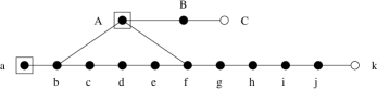
Figure 1: The underlying entanglement graph for the $\mathop{\wedge}\hskip-1.72218ptU$ pattern.

Extended standardisation yields:

$$\begin{array}[c]{lllllllllllllll}Z_{k}^{s_{i}+s_{g}+s_{e}+s_{c}+s_{a}}X_{k}^{s_{j}+s_{h}+s_{f}+s_{d}+s_{b}}X_{C}^{s_{B}}Z_{C}^{s_{A}+s_{e}+s_{c}}\\ {M}_{B}^{0}{M}_{A}^{-\alpha^{\prime}}{M}_{j}^{0}[{M}_{i}^{\beta-\pi}]^{s_{h}+s_{f}+s_{d}+s_{b}}[{M}_{h}^{-\frac{\gamma}{2}}]^{s_{g}+s_{e}+s_{c}+s_{a}}[{M}_{g}^{\frac{\pi}{2}}]^{s_{f}+s_{d}+s_{b}}\\ {M}_{f}^{0}[{M}_{e}^{-\frac{\pi}{2}}]^{s_{d}+s_{b}}[{M}_{d}^{\frac{\gamma}{2}}]^{s_{c}+s_{a}}[{M}_{c}^{\frac{\pi-\delta-\beta}{2}}]^{s_{b}}{M}_{b}^{0}{M}_{a}^{\frac{-\beta+\delta+\pi}{2}}\\ E_{BC}E_{AB}E_{jk}E_{ij}E_{hi}E_{gh}E_{fg}E_{Af}E_{ef}E_{de}E_{cd}E_{bc}E_{ab}E_{Ab}\end{array}$$

Figure 2 shows the dependency structure of the resulting standard pattern for $\mathop{\wedge}\hskip-1.72218ptU$, and one sees it has depth complexity $7$.

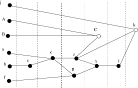
Figure 2: The dependency graph for the standard $\mathop{\wedge}\hskip-1.72218ptU$ pattern.

7 The no dependency theorems

From standardization we can also infer results related dependencies. We start with a simple observation which is a direct consequence of standardisation.

Lemma 6

Let $\mathfrak{P}$ be a pattern implementing some unitary $U$, and suppose $\mathfrak{P}$’s command sequence has measurements only of the $M^{x}$ and $M^{y}$ kind, then $U$ has a standard implementation, having only independent measurements, all being of the $M^{x}$ and $M^{y}$ kind (therefore of depth complexity at most 2).

Write $\mathfrak{P}^{\prime}$ for the standard pattern associated to $\mathfrak{P}$. By equations (15) and (16), the $X$-actions can be eliminated from $\mathfrak{P}^{\prime}$, and then $Z$-actions can be eliminated by using the extended calculus. The final pattern still implements $U$, has no longer any dependent measurements, and has therefore depth complexity at most 2. $\Box$

Theorem 1

Let $U$ be a unitary operator, then $U$ is in the Clifford group iff there exists a pattern $\mathfrak{P}$ implementing $U$, having measurements only of the $M^{x}$ and $M^{y}$ kind.

The “only if” direction is easy, since we have seen in the example section, standard patterns for $\mathop{\wedge}\hskip-1.72218ptX$, $H$ and $P(\frac{\pi}{2})$ which had only $M^{x}$ and $M^{y}$ measurements. Hence any Clifford operator can be implemented by a combination of these patterns. By the lemma above, we know we can actually choose these patterns to be standard.

For the “if” direction, we prove that $U$ belongs to the normaliser of the Pauli group, and hence by definition to the Clifford group. In order to do so we use the standard form of $\mathfrak{P}$ written as $\mathfrak{P}^{\prime}=C_{\mathfrak{P}^{\prime}}M_{\mathfrak{P}^{\prime}}E_{\mathfrak{P}^{\prime}}$ which still implements $U$, and has only $M^{x}$ and $M^{y}$ measurements.

Let $i$ be an input qubit, and consider the pattern $\mathfrak{P}^{\prime\prime}={\mathfrak{P}}C_{i}$, where $C_{i}$ is either $X_{i}$ or $Z_{i}$. Clearly $\mathfrak{P}^{\prime\prime}$ implements $UC_{i}$. First, one has:

$$\begin{array}[c]{lllllllllllllll}C_{\mathfrak{P}^{\prime}}M_{\mathfrak{P}^{\prime}}E_{\mathfrak{P}^{\prime}}C_{i}&\Rightarrow_{EC}^{\star}&C_{\mathfrak{P}^{\prime}}M_{\mathfrak{P}^{\prime}}C^{\prime}E_{\mathfrak{P}^{\prime}}\end{array}$$

for some non-dependent sequence of corrections $C^{\prime}$, which, up to free commutations can be written uniquely as $C^{\prime}_{O}C^{\prime\prime}$, where $C^{\prime}_{O}$ applies on output qubits, and therefore commutes to $M_{\mathfrak{P}^{\prime}}$, and $C^{\prime\prime}$ applies on non-output qubits (which are therefore all measured in $M_{\mathfrak{P}^{\prime}}$). So, by commuting $C^{\prime}_{O}$ both through $M_{\mathfrak{P}^{\prime}}$ and $C_{\mathfrak{P}^{\prime}}$ (up to a global phase), one gets:

$$\begin{array}[c]{lllllllllllllll}C_{\mathfrak{P}^{\prime}}M_{\mathfrak{P}^{\prime}}C^{\prime}E_{\mathfrak{P}^{\prime}}&\Rightarrow^{\star}&C^{\prime}_{O}C_{\mathfrak{P}^{\prime}}M_{\mathfrak{P}^{\prime}}C^{\prime\prime}E_{\mathfrak{P}^{\prime}}\end{array}$$

Using equations (15), (16), and the extended calculus to eliminate the remaining $Z$-actions, one gets:

$$\begin{array}[c]{lllllllllllllll}M_{\mathfrak{P}^{\prime}}C^{\prime\prime}&\Rightarrow_{MC,S}^{\star}&SM_{\mathfrak{P}^{\prime}}\end{array}$$

for some product $S=\prod_{\{j\in J\}}S_{j}^{1}$ of constant shiftings, applying to some subset $J$ of the non-output qubits. So:

$$\begin{array}[c]{lllllllllllllll}C^{\prime}_{O}C_{\mathfrak{P}^{\prime}}M_{\mathfrak{P}^{\prime}}C^{\prime\prime}E_{\mathfrak{P}^{\prime}}&\Rightarrow^{\star}&C^{\prime}_{O}C_{\mathfrak{P}^{\prime}}SM_{\mathfrak{P}^{\prime}}E_{\mathfrak{P}^{\prime}}\\ &\Rightarrow^{\star}&C^{\prime}_{O}C^{\prime\prime}_{O}C_{\mathfrak{P}^{\prime}}M_{\mathfrak{P}^{\prime}}E_{\mathfrak{P}^{\prime}}\end{array}$$

where $C^{\prime\prime}_{O}$ is a further constant correction obtained by shifting $C_{\mathfrak{P}^{\prime}}$ with $S$. This proves that $\mathfrak{P}^{\prime\prime}$ also implements $C^{\prime}_{O}C^{\prime\prime}_{O}U$, and therefore $UC_{i}=C^{\prime}_{O}C^{\prime\prime}_{O}U$ which completes the proof, since $C^{\prime}_{O}C^{\prime\prime}_{O}$ is a non dependent correction. $\Box$

The only if part of this theorem already appears in previous work [RBB03, p.18].

We can further prove that dependencies are crucial for the universality of the model. Observe first that if a pattern has no measurements, and hence no dependencies, then it follows from (D2) that $V=O$, i.e., all qubits are outputs. Therefore computation steps involve only $X$, $Z$ and $\mathop{\wedge}\hskip-1.72218ptZ$, and it is not surprising that they compute a unitary which is in the Clifford group. The general argument essentially consists in showing that when there are measurements, but still no dependencies, then the measurements are playing no part in the result.

Theorem 2

Let $\mathfrak{P}$ be a pattern implementing some unitary $U$, and suppose $\mathfrak{P}$’s command sequence doesn’t have any dependencies, then $U$ is in the Clifford group.

Write $\mathfrak{P}^{\prime}$ for the standard pattern associated to $\mathfrak{P}$. Since rewriting is sound, $\mathfrak{P}^{\prime}$ still implements $U$, and since rewriting never creates any dependency, it still has no dependencies. In particular, the corrections one finds at the end of $\mathfrak{P}^{\prime}$, call them $C$, bear no dependencies. Erasing them off $\mathfrak{P}^{\prime}$, results in a pattern $\mathfrak{P}^{\prime\prime}$ which is still standard, still deterministic, and implementing $U^{\prime}:=C^{\star}U$.

Now how does the pattern $\mathfrak{P}^{\prime\prime}$ run on some input $\phi$ ? First $\phi\otimes{|}\hskip-1.72218pt+\ldots+\rangle$ goes by the entanglement phase to some $\psi\in\mathfrak{H}_{V}$, and is then subjected to a sequence of independent 1-qubit measurements. Pick a basis $\mathcal{B}$ spanning the Hilbert space generated by the non-output qubits $\mathfrak{H}_{V\setminus O}$ and associated to this sequence of measurements.

Since $\mathfrak{H}_{V}=\mathfrak{H}_{O}\otimes\mathfrak{H}_{V\setminus O}$ and $\mathfrak{H}_{V\setminus O}=\oplus_{\phi_{b}\in B}[\phi_{b}]$, where $[\phi_{b}]$ is the linear subspace generated by $\phi_{b}$, by distributivity, $\psi$ uniquely decomposes as:

$$\begin{array}[c]{lllllllllllllll}\psi=\sum_{\phi_{b}\in\mathcal{B}}\phi_{b}\otimes x_{b}\end{array}$$

where $\phi_{b}$ ranges over $\mathcal{B}$, and $x_{b}\in\mathfrak{H}_{O}$. Now since $\mathfrak{P}^{\prime\prime}$ is deterministic, there exists an $x$, and scalars $\lambda_{b}$ such that $x_{b}=\lambda_{b}x$. Therefore $\psi$ can be written $\psi^{\prime}\otimes x$, for some $\psi^{\prime}$. It follows in particular that the output of the computation will still be $x$ (up to a scalar), no matter what the actual measurements are. One can therefore choose them to be all of the ${M}^{x}$ kind, and by the preceding theorem $U^{\prime}$ is in the Clifford group, and so is $U=CU^{\prime}$, since $C$ is a Pauli operator. $\Box$

From this section, we conclude in particular that any universal set of patterns has to include dependencies (by the preceding theorem), and also needs to use measurements $M^{\alpha}$ where $\alpha\neq 0$ modulo $\frac{\pi}{2}$ (by the theorem before). This is indeed the case for the universal set $\mathfrak{J}(\alpha)$ and $\mathop{\wedge}\hskip-1.72218pt{\mathfrak{Z}}$.

8 Conclusion

We presented a calculus for 1-qubit measurement based quantum computing. We have seen that pattern combinations allow for a structured proof of universality, which also results in parsimonious implementations. We have shown further that our calculus defines a quadratic-time standardisation algorithm transforming any pattern to a standard form where entanglement is done first, then measurements, then local corrections. And finally, we have inferred from this procedure that patterns with no dependencies, or using only Pauli measurements, may only implement unitaries in the Clifford group.

An obvious question is whether one can extend these ideas to other measurement based models, perhaps based on different families of entanglement operators, more general measurements and other types of local corrections. This is a matter which we wish to explore further. For now, it is already clear that both the notation and the calculus can be extended to the teleportation model which is based on 2-qubit measurements. This actually shows that teleportation models are embeddable in the one-way model in a very strong sense. We will return to this particular question elsewhere.

We also feel that the methods explored here can be stretched further and made to be relevant to the study of error propagation and error correcting, but this demands using mixed states, and interpreting patterns as cp-maps.

Finally, there is also a clear reading of dependencies as classical communications, while local corrections can be thought of as local quantum operations in a multipartite scenario. Along this reading, standardisation pushes non-local operations to the beginning of a distributed computation, and it seems the measurement calculus could prove useful in the area of quantum protocols.

9 Appendix

We prove here that standardisation has indeed the properties quoted in the body of the paper. First, we need a lemma:

Lemma 7 (Termination)

For all $\mathfrak{P}$, there exists finitely many $\mathfrak{P}^{\prime}$ such that $\mathfrak{P}\Rightarrow^{\star}\mathfrak{P}^{\prime}$.

Suppose $\mathfrak{P}$ has command sequence $A_{n}\ldots A_{1}$, and define for $A_{i}=E_{ij}$ $d(A_{i})=i$, and for $A_{j}=X_{u}^{s}$, $d(A_{j})=n-j$. Define further:

$$\begin{array}[c]{lllllllllllllll}d(\mathfrak{P})&=&(\sum_{E\in\mathfrak{P}}d(E),\sum_{C\in\mathfrak{P}}d(C))\end{array}$$

This measure decreases lexicographically under rewriting, in other words $\mathfrak{P}\Rightarrow\mathfrak{P}^{\prime}$ implies $d(\mathfrak{P})>d(\mathfrak{P}^{\prime})$, where $<$ is the lexicographic ordering on $\mathbb{N}^{2}$. Let us inspect all cases. First when one applies $EC$, then the first coordinate strictly diminishes (the second does not always, because of the duplication involved if $C=X$); when $MC$, the second strictly diminishes and the first stays the same or diminishes; when $EA$, the first strictly diminishes (because we dropped the case when $A$ is itself an $E$), and maybe the second; when $AC$, the second strictly diminishes, and the first stays the same or diminishes (when $A=E$).

Therefore, all rewritings are finite, and since the system is finitely branching (there are no more than $n$ possible single step rewrites on a given sequence of length $n$), we get the statement of the theorem. $\Box$

It is not to difficult to strengthen the result above, by showing that the longest possible rewriting of $\mathfrak{P}$ is quadratic in $n$, where $n$ is the length of $\mathfrak{P}$’s command sequence.

Say $\mathfrak{P}$ is standard if for no $\mathfrak{P}^{\prime}$, $\mathfrak{P}\Rightarrow\mathfrak{P}^{\prime}$.

Proposition 8 (Standardisation)

For all $\mathfrak{P}$, there exists a unique standard $\mathfrak{P}^{\prime}$, such that $\mathfrak{P}\Rightarrow^{\star}\mathfrak{P}^{\prime}$, and $\mathfrak{P}^{\prime}$ satisfies the (EMC) condition.

Since the rewriting system is terminating, confluence follows from local confluence (meaning whenever two rewritings can be applied, one can rewrite further both transforms to a same third expression). Then, uniqueness of the standard form is an easy consequence (actually, for terminating rewriting systems, unicity of standard forms and confluence are equivalent). Looking for critical pairs, that is occurrences of three successive commands where two rules can be applied simultaneously, one finds that there are only two types: $E_{ij}M_{k}C_{k}$ with $i$, $j$ and $k$ all distinct, and $E_{ij}M_{k}C_{l}$ with $k$ and $l$ distinct. In both cases local confluence is easily verified.

Suppose now ${\mathfrak{P}^{\prime}}$ does not satisfy (EMC). Then, either there is a pattern $EA$ with $A$ not of type $E$, or there is a pattern $AC$ with $A$ not of type $C$. In the former case, $E$ and $A$ must operate on overlapping qubits, else one may apply a free commutation rule, and $A$ may not be a $C$ since in this case one may apply an $EC$ rewrite. The only remaining case in when $A$ is of type $M$, overlapping $E$’s qubits, but this is what condition (D1) forbids, and since (D1) is preserved under rewriting, this contradicts the assumption. The latter case is even simpler. $\Box$

9.1 Discussion

This is what we wanted, namely we have shown that under rewriting any pattern can be put in (EMC) form. We actually proved a bit more, namely that the standard form obtained is unique.

However, one has to be a bit careful about the significance of this additional piece of information. Note first that unicity is obtained because we dropped the $CC$ free commutations, and all $EE$ commutations, thus having a very rigid notion of command sequence. One cannot put them back as rewriting rules, since they obviously ruin termination and uniqueness of standard forms.

A reasonable thing to do, would be to take this set of equations as generating an equivalence relation on command sequences, call it $\equiv$, and hope to strengthen the results obtained so far, by proving that all reachable standard forms are equivalent.

But this is too naive a strategy, since $E_{12}X_{1}X_{2}\equiv E_{12}X_{2}X_{1}$, and:

$$\begin{array}[c]{lllllllllllllll}E_{12}X_{1}^{s}X_{2}^{t}&\Rightarrow^{\star}&X_{1}^{s}Z_{2}^{s}X_{2}^{t}Z_{1}^{t}E_{12}\\ &\equiv&X_{1}^{s}Z_{1}^{t}Z_{2}^{s}X_{2}^{t}E_{12}\end{array}$$

obtaining an expression which is not symmetric in $1$ and $2$. To conclude, one has to extend $\equiv$ to include the additional equivalence $X_{1}^{s}Z_{1}^{t}\equiv Z_{1}^{t}X_{1}^{s}$, which fortunately is sound since these two operators are equal up to a global phase. We conjecture that this enriched equivalence is preserved.

References

- [AL04] P. Aliferis and D. W. Leung. Computation by measurements: a unifying picture. Quant-ph/0404082, April 2004.
- [BR04] D. E. Browne and T. Rudolph. Efficient linear optical quantum computation. Quant-ph/0405157, 2004.
- [CAJ04] S.R. Clark, C. Moura Alves, and D. Jaksch. Controlled generation of graph states for quantum computation in spin chains. Quant-ph/0406150, 2004.
- [DKP04] V. Danos, E. Kashefi, and P. Panangaden. Robust and parsimonious realisations of unitaries in the one-way model. Quant-ph/0411071, 2004.
- [HEB04] M. Hein, J. Eisert, and H.J. Briegel. Multi-party entanglement in graph states. Phys. Rev. A, 69:62311–62333, 2004.
- [ND04] M. A. Nielsen and C. M. Dawson. Fault-tolerant quantum computation with cluster states. Quant-ph/0405134, 2004.
- [Nie04] M. A. Nielsen. Optical quantum computation using cluster states. quant-ph/0402005, 2004.
- [RBB03] R. Raussendorf, D. E. Browne, and H. J. Briegel. Measurement-based quantum computation on cluster states. Physical Review, A 68(022312), 2003.