Quantum computation and analysis of Wigner and Husimi functions:
toward a quantum image treatment

Abstract

We study the efficiency of quantum algorithms which aim at obtaining phase space distribution functions of quantum systems. Wigner and Husimi functions are considered. Different quantum algorithms are envisioned to build these functions, and compared with the classical computation. Different procedures to extract more efficiently information from the final wave function of these algorithms are studied, including coarse-grained measurements, amplitude amplification and measure of wavelet-transformed wave function. The algorithms are analyzed and numerically tested on a complex quantum system showing different behavior depending on parameters, namely the kicked rotator. The results for the Wigner function show in particular that the use of the quantum wavelet transform gives a polynomial gain over classical computation. For the Husimi distribution, the gain is much larger than for the Wigner function, and is bigger with the help of amplitude amplification and wavelet transforms. We also apply the same set of techniques to the analysis of real images. The results show that the use of the quantum wavelet transform allows to lower dramatically the number of measurements needed, but at the cost of a large loss of information.

I I.Introduction

In the recent years, the study of quantum information nielsen has attracted more and more interest. In this field, quantum mechanics is used to treat and manipulate information. Important applications are quantum cryptography, quantum teleportation and quantum computation. The latter takes advantage of the laws of quantum mechanics to perform computational tasks sometimes much faster than classical devices. A famous example is provided by the problem of factoring large integers, useful for public-key cryptography, which can be solved with exponential efficiency by Shor’s algorithm shor . Another example is the search of an unstructured list, which was shown by Grover grover to be quadratically faster on quantum devices. In parallel, investigations of the simulation of quantum systems on quantum computers showed that the evolution of a complex wave function can be simulated efficiently for an exponentially large Hilbert space with polynomial resources lloyd ; schack ; GS ; song ; complex ; pomeransky . Still, there are many open questions which remain unanswered. In particular, it is not always clear how to perform an efficient extraction of information from such a complex quantum mechanical wave function once it has been evolved on a quantum computer. More generally, the same problem appears for quantum algorithms manipulating large amount of classical data.

In the present paper, we study different algorithmic processes which perform this task. We focus on the phase space distribution (Wigner and Husimi functions) wigner ; husimi These functions provide a two-dimensional picture of a one-dimensional wave function, and can be compared directly with classical phase space distributions. They have also been shown in Levi ; harper to be stable with respect to various quantum computer error models. Different phase space representation which can be implemented efficiently on a quantum computer will be explored, first the discrete Wigner transform, for which an original algorithm will be presented, and then a Husimi-like transform, first introduced in this context in frahm . Recent proposals frahm ; pazwigner ; saraceno gave methods to measure or construct Wigner and Husimi functions on a quantum computer, using for example phase space tomography. These method will be analyzed and compared with new strategies, in order to identify the most efficient algorithms. Different techniques will be tested in order to extract information, namely measure of an ancilla qubit, measurement of all qubits, coarse grained measurement, and the use of amplitude amplification amplification . In addition, we will analyze the use of the wavelet transform to compress information and minimize the number of measurements. Indeed, wavelet transforms Daub ; meyer are used in a large number of applications involving classical data treatment, in particular they allow to reach large compression rates for classical images in standards like MPEG. Quantum wavelet transforms have been built and implemented WT1 ; WT2 ; WT3 ; terraneo , and it was shown that they can be applied on an exponentially large vector in a polynomial number of operations. Numerical computations will enable us to quantify the efficiency of each method for a specific complex quantum system, namely the kicked rotator. In general, it will be shown that a polynomial gain can be reached with several strategies. Since a quantum phase space distribution can be considered as an example of a two-dimensional picture, we discuss in a subsequent section the use of the same techniques to treat images encoded on the wave function of a quantum computer, in a way similar to what is done in classical image analysis. This for example could be applied to images transmitted through quantum imaging kolobov .

II II. Quantum phase space distributions for a chaotic quantum map

Classical Hamiltonian mechanics is built in phase space, dynamics being governed by Hamilton’s equation of motion. Classical motion can be described through the evolution of phase space (Liouville) distributions. On the other hand, phase space is a peculiar notion in quantum mechanics since $p$ and $q$ do not commute. A wave function is naturally described in a Hilbert space, for example position alone or momentum alone. Nevertheless, it has been known since a long time that it is possible to define functions of $p$ and $q$ which can be thought as quantum phase space distributions. The most commonly used is the Wigner function wigner , defined for the wave function $\psi$ of a continuous system by:

$$W(p,q)=\int\frac{e^{-\frac{i}{\hbar}p.q^{\prime}}}{\sqrt{2\pi\hbar}}\psi(q+\frac{q^{\prime}}{2})^{*}\psi(q-\frac{q^{\prime}}{2})dq^{\prime}$$ (1)

This function involves the two variables position $q$ and momentum $p$ in a symmetric way (although it is not immediately apparent in the formula (1)), and shares some properties with classical phase space probability distributions. Indeed, it is a real function, and satisfies $\int W(p,q)dq=|\psi(p)|^{2}$ and $\int W(p,q)dp=|\psi(q)|^{2}$. However, it cannot be identified with a probability distribution since it can take negative values. The Wigner function has been measured experimentally in atomic systems, and such negative values have been reported negative .

Although the Wigner function can take negative values, it can be shown that coarse graining this function over cells of size $\hbar$ always leads to nonnegative values. Therefore a smoothing of (1) by appropriate functions will lead to a function of $p$ and $q$ with no negative values. An example of such a function is given by the Husimi distribution (see e.g. husimi ) which uses a Gaussian smoothing. A further example using another smoothing function was discussed in frahm .

In the following sections, we will study the evaluation of such quantum phase space distributions of wave functions on a quantum computer. This will be performed using a specific example, namely the kicked rotator model. This system corresponds to the quantization of the Chirikov standard map qchaos ; lichtenberg $\bar{n}=n+k\sin{\theta};\;\;\;\bar{\theta}=\theta+T\bar{n}$ where $(n,\theta)$ are the conjugated (action-angle) variables.

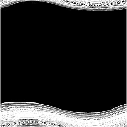
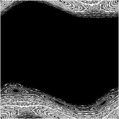
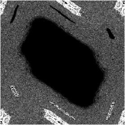
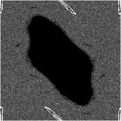
Figure 1: Classical phase space distribution for the standard map with $K=0.5$ (top left), $K=0.9$ (top right), $K=1.5$ (bottom left), $K=2$ (bottom right). Black is zero probability, white is maximal probability. As initial state we chose a uniform distribution on the set $-\pi\leq p\leq-3/4\pi$, $0\leq x\leq 2\pi$, and $1000$ iterations of the standard map were performed.

The classical standard map depends only on the parameter $K=kT$. The system undergoes a transition from integrability ($K=0$) to more and more developed chaos when $K$ increases, following the Kolmogorov-Arnold-Moser theorem. Chaotic zones get larger and larger until the value $K=K_{g}\approx 0.9716...$ is reached, where global chaos sets in, but a complex hierarchical structure of integrable islands surrounded by chaotic layers is still present. For $K\gg K_{g}$, the chaotic part covers most of the phase space. This system has been used for example as a model of particle confinement in magnetic traps, beam dynamics in accelerators or comet trajectories lichtenberg . Its phase space is a cylinder (periodicity in $\theta$), and since the map is periodic in $n$ with period $2\pi/T$, phase space structures repeat themselves in the $n$ direction on each cell of size $2\pi/T$. Fig.1 shows one such phase space cell for various values of the parameter $K$, showing the different regimes from quasi-integrability (many invariant curves preventing transport in the momentum direction) to a mixed regime with a large chaotic domain.

The quantum version of the standard map qchaos gives a unitary operator acting on the wave function $\psi$ through:

$$\bar{\psi}=\hat{U}\psi=e^{-ik\cos{\hat{\theta}}}e^{-iT\hat{n}^{2}/2}\psi,$$ (2)

where $\hat{n}=-i\partial/\partial\theta$, $\hbar=1$, and $\psi(\theta+2\pi)=\psi(\theta)$.

The quantum dynamics (2) depends on the two parameters $k$ and $T$, $T$ playing the role of an effective $\hbar$. The classical limit is $k\rightarrow\infty$, $T\rightarrow 0$ while keeping $K=kT=$ constant.

This quantum kicked rotator (2) is described by quite simple equations, making it practical for numerical simulations and quantum computing. Nevertheless, it displays a wealth of different behaviors depending on the values of the parameters. Indeed, classical dynamics undergoes a transition from integrability to fully developed chaos with intermediate mixed phases between these two regimes. Wave functions show complex structures related to the classical phase space corresponding to these different cases. In addition, for large $K$ where classical dynamics is strongly chaotic, quantum interference can lead to exponential localization of wave functions. This phenomenon is related to the Anderson localization of electrons in solids, and therefore enables to study this important solid state problem, which is still the subject of active research. The kicked rotator can also model the microwave ionization of Rydberg atoms IEEE , and has been experimentally realized with cold atoms raizen . For all these reasons, it has been the subject of many studies, and can be considered as a paradigmatic model of quantum chaos.

In GS ; Levi it was shown that evolving a $N$-dimensional wave function through the map (2) can be done with only $O(\log N)$ qubits and $O((\log N)^{3})$ operations on a quantum computer (compare with $O(N\log N)$ operations for the same simulation on a classical computer). Another quantum algorithm developed in pomeransky enables to perform the same quantum evolution (albeit approximately) with $O((\log N)^{2})$ operations. This system can therefore be simulated efficiently on a quantum computer, and can be used as a good test ground for assessing the complexity of various quantum algorithms for quantum phase space distributions.

In the following sections, we will study the efficiency of various quantum algorithms to obtain various information about the quantum phase space distribution functions. The simulation of a quantum system on a quantum computer based on qubits implies that the system is effectively discrete and finite. We therefore close the phase space in the momentum direction through periodic boundary conditions. We will concentrate on the regime where $T=2\pi/N$, $N$ being the Hilbert space dimension. This implies that the phase space contains only one classical cell, and increasing the number of qubits at $K$ constant decreases the effective $\hbar$ keeping the classical dynamics constant. Different $K$ values enable to probe various dynamical regimes, from integrability to chaos. The localization length in this regime becomes quickly larger than the system size for small number of qubits, thus allowing to explore the complexity of a chaotic wave function. Indeed, in the localized regime, the most important information resides not so much in such distributions, but in the localization properties, and their measurement on a quantum computer was already analyzed in loclength ; harper .

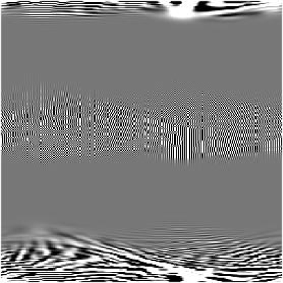
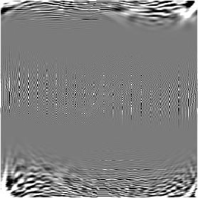
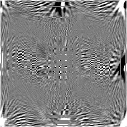
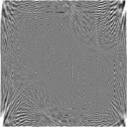
Figure 2: Wigner function for the quantum kicked rotator with parameters of Fig.1 $K=0.5$ (top left), $K=0.9$ (top right), $K=1.5$ (bottom left), $K=2$ (bottom right). Here $T=2\pi/N$, where $N=2^{n_{q}}$, with $n_{q}=7$. The whole Wigner function (on a $2N\times 2N$ lattice) is plotted. White marks positive maximal values, black negative values. Initial state is uniformly spread on the set $0\leq n<N/8$ (corresponding to the initial classical distribution in Fig.1) (this state can be built efficiently from $|n=0\rangle$ by $n_{q}-3$ Hadamard gates), and Wigner function is computed after $1000$ iterations of (2).

For such a quantum system on a $N$ dimensional Hilbert space, the general formalism of Wigner functions should be adapted. In particular, it is known that it should be constructed on $2N\times 2N$ points (see e.g. discrete ). For the kicked rotator, the formula for the discrete Wigner function is:

$$W(\Theta,n)=\sum_{m=0}^{N-1}\frac{e^{-\frac{2i\pi}{N}n(m-\Theta/2)}}{2N}\psi(\Theta-m)^{*}\psi(m),$$ (3)

with $\Theta=\frac{N\theta}{2\pi}$.

The Wigner function provides a pictorial representation of a wave function which can be compared with the classical phase space distribution, (see example in Fig.2), although quantum oscillations are present.

III III. Measuring the Wigner distribution

In pazwigner the first quantum algorithm was set up which enables to measure the value of the Wigner function at a given phase space point. The algorithm adds one ancilla qubit to the system and proceeds by applying one Hadamard gate to the ancilla qubit, then a certain operator $U(\Theta,n)$ is applied to the system controlled by the value of the ancilla qubit. After a last Hadamard gate is applied to the ancilla, its expectation value is $<\sigma^{z}>=Re[Tr(U(\Theta,n)\rho)]=2NW(\Theta,n)$ where $\rho$ is the density matrix and $N=2^{n_{q}}$ is the dimension of the Hilbert space. One iteration of this process requires only a logarithmic number of gates. Nevertheless, the total complexity of the algorithm may be much larger, since measuring $<\sigma^{z}>$ may require a very large number of measurements. This can be probed only through careful estimation of the asymptotic behavior of individual values of the Wigner function.

A drawback of the approach of pazwigner is that it does not allow easily further treatment on the Wigner function which may improve the total complexity of the algorithm. To this aim, the simplest way is to build explicitly the Wigner transform of the wave function as amplitudes of a register. This enables to use additional tools (amplitude amplification, wavelet transforms) which may increase the speedup over classical computation, as we will see.

Such an explicit construction of the Wigner function directly on the registers of the quantum computer is indeed possible in the following way. To get the Wigner function of $\hat{U}^{t}|\psi_{0}\rangle$ ($t$ iterations of an original wave function $|\psi_{0}\rangle$ through (2)), we start from an initial state (for example in $n$ representation) $|\psi_{0}\rangle\otimes|\psi^{*}_{0}\rangle$ $=\sum_{i=0}^{N-1}a_{i}|n_{i}\rangle\otimes\sum_{j=0}^{N-1}a^{*}_{j}|n_{j}\rangle$ $=\sum_{i=0}^{N-1}\sum_{j=0}^{N-1}a_{i}a^{*}_{j}|n_{i}\rangle|n_{j}\rangle$. This needs $2n_{q}$ qubits to hold the values of the wave function on a $N$-dimensional Hilbert space, where $N=2^{n_{q}}$. Then we apply the algorithm implementing the kicked rotator evolution operator $\hat{U}$ developed in GS to each subsystem independently. This operator can be described as multiplication by phases followed by a quantum Fourier transform (QFT). The multiplication by phases of each coefficient keeps the factorized structure. The QFT mixes only states with the same value of the other register attached, and therefore also keeps the factorized form. Let us see how it works for one iteration:

$$\sum_{i=0}^{N-1}\sum_{j=0}^{N-1}a_{i}a^{*}_{j}|n_{i}\rangle|n_{j}\rangle\rightarrow\sum_{i=0}^{N-1}\sum_{j=0}^{N-1}e^{-iTn_{i}^{2}/2}a_{i}a^{*}_{j}|n_{i}\rangle|n_{j}\rangle$$

(multiplication by $e^{-iT\hat{n_{i}}^{2}/2}$)

$$=\sum_{j=0}^{N-1}(\sum_{i=0}^{N-1}e^{-iTn_{i}^{2}/2}a_{i}|n_{i}\rangle)a^{*}_{j}|n_{j}\rangle\rightarrow\sum_{j=0}^{N-1}(\sum_{i=0}^{N-1}b_{i}|\theta_{i}\rangle)a^{*}_{j}|n_{j}\rangle$$

(QFT with respect to $n_{i}$)

$$\rightarrow\sum_{j=0}^{N-1}(\sum_{i=0}^{N-1}e^{-ik\cos{\theta_{i}}}b_{i}|\theta_{i}\rangle)a^{*}_{j}|n_{j}\rangle$$

(multiplication by $e^{-ik\cos{\theta_{i}}}$)

$$\rightarrow\sum_{j=0}^{N-1}(\sum_{i=0}^{N-1}c_{i}|n_{i}\rangle)a^{*}_{j}|n_{j}\rangle$$

(QFT with respect to $\theta_{i}$)

$$=(\sum_{i=0}^{N-1}c_{i}|n_{i}\rangle)\otimes(\sum_{j=0}^{N-1}a^{*}_{j}|n_{j}\rangle)=\hat{U}|\psi_{0}\rangle\otimes|\psi^{*}_{0}\rangle$$

We can thus get $\hat{U}^{t}|\psi_{0}\rangle\otimes\hat{U}^{*t}|\psi^{*}_{0}\rangle$ by applying the process several times. This can be done in a number of gates polynomial in $n_{q}$ ($O(tn_{q}^{3})$ if we use the algorithm of GS for implementing $\hat{U}$).

From such a state it is possible to build efficiently the state $\sum_{\theta,n}W(\theta,n)|\theta\rangle|n\rangle$. Indeed, building the Wigner transform can be done through a partial Fourier transform. To see this, we start from the state in $\theta$ representation, i.e. $|\psi\rangle\otimes|\psi^{*}\rangle$= $\sum_{\theta,\theta^{\prime}}\psi(\theta)\psi^{*}(\theta^{\prime})|\theta\rangle|\theta^{\prime}\rangle$. Then we add an extra qubit to the first register (needed to get values of $\theta+\theta^{\prime}$ between $0$ and $2N-1$) and realize the transformation:

$\sum_{\theta,\theta^{\prime}}\psi(\theta)\psi^{*}(\theta^{\prime})|\theta\rangle|\theta^{\prime}\rangle$ $\rightarrow\sum_{\theta,\theta^{\prime}}\psi(\theta)\psi^{*}(\theta^{\prime})|\theta+\theta^{\prime}\rangle|\theta^{\prime}\rangle$ (addition)

Let us call $\Theta=\theta+\theta^{\prime}$; then the state can be written $\sum_{\Theta,\theta^{\prime}}\psi(\Theta-\theta^{\prime})\psi^{*}(\theta^{\prime})|\Theta\rangle|\theta^{\prime}\rangle$ Then we realize a QFT of the second register only. The result is: $\sum_{\Theta}\sum_{n}(\sum_{\theta^{\prime}}e^{-\frac{2i\pi}{N}n\theta^{\prime}}\psi(\Theta-\theta^{\prime})\psi^{*}(\theta^{\prime}))|\Theta\rangle|n\rangle$ =$2\sqrt{N}\sum_{\Theta}\sum_{n}W(\Theta,n)e^{-\frac{2i\pi}{N}n\Theta/2}|\Theta\rangle|n\rangle$ where $\Theta$ varies from $0$ to $2N-1$ and $n$ from $0$ to $N-1$. To get the Wigner function on a $2N\times 2N$ grid, we need first to add an extra qubit in the state $|0\rangle$ and apply a Hadamard gate to it. If we interpret it as the most significant digit of $n$, the resulting state is $\sqrt{2N}\sum_{\Theta}\sum_{n=0}^{N-1}W(\Theta,n)e^{-\frac{2i\pi}{N}n\Theta/2}|\Theta\rangle|n\rangle+\sqrt{2N}\sum_{\Theta}\sum_{n=N}^{2N-1}W(\Theta,n)e^{-\frac{2i\pi}{N}(n-N)\Theta/2}|\Theta\rangle|n\rangle$. The final step consists in multiplying by the phases $e^{-\frac{2i\pi}{N}n\Theta/2}$ and $e^{-\frac{2i\pi}{N}(n-N)\Theta/2}$, which can be made by $n_{q}^{2}$ application of two-qubit gates (controlled phase-shifts). The final state is

$$|\psi_{f}\rangle=\sqrt{2N}\sum_{\Theta=0}^{2N-1}\sum_{n=0}^{2N-1}W(\Theta,n)|\Theta\rangle|n\rangle$$ (4)

One can check that the normalization is correct since it is known in general that $\sum_{\Theta=0}^{2N-1}\sum_{n=0}^{2N-1}W(\Theta,n)^{2}=1/2N$.

The advantage of this procedure in comparison to the one in pazwigner resides in the fact that individual values of the Wigner function are now encoded in the components of the wave function. This is in general a natural way to encode an image on a wave function: each basis vector corresponding to a position in phase space is associated with a coefficient giving the amplitude at this location. This way of encoding the Wigner function enables to perform some further operations to extract information efficiently through quantum measurements. We will envision three different strategies: direct measurements of each qubit, amplitude amplification and wavelet transform. The data of Fig.3-6 will enable us to compare these different strategies for different physical regimes of the kicked rotator model, with various levels of chaoticity. The quantity plotted is the inverse participation ratio (IPR). For a wave function $|\psi\rangle=\sum_{i=1}^{N}\psi_{i}|i\rangle$, where $|i\rangle$ is some basis, the inverse participation ratio is $\sum|\psi_{i}|^{2}/(\sum|\psi_{i}|^{4})$ and measures the number of significant components in the basis $|i\rangle$. The Wigner function verifies the sum rules $\sum W_{i}=1$ and $\sum W_{i}^{2}=\frac{1}{N}$. Following Levi we are lead by analogy to define the inverse participation ratio for the Wigner function, by the formula $\xi=1/(N^{2}\sum W_{i}^{4})$. If the Wigner function is composed of $N$ components of equal weights $1/N$, then $\xi=N$, whereas $N^{2}$ components of equal weights (in absolute value) $1/N^{3/2}$ give $\xi=N^{2}$. Thus the IPR $\xi$ gives an estimate of the number of the main components of the Wigner function.

Figure 3: Main plot: scaling of the IPR $\xi$ vs. $n_{q}$ for the Wigner function (empty squares) and for the wavelet transform of the Wigner function (full squares). The full straight lines represent the law $N^{2}$, $N=2^{n_{q}}$. Here $K=0.5$. In the inset, the ratio $R$ between IPR of Wigner function and wavelet transformed Wigner function is plotted. Parameters, number of iterations and initial state are the same as in Fig.2.

Figure 4: Main plot: scaling of the IPR $\xi$ vs. $n_{q}$ for the Wigner function (empty squares) and for the wavelet transform of the Wigner function (full squares). The full straight line represents the law $N^{1.75}$, while the dashed line represents $N^{2}$, $N=2^{n_{q}}$. Here $K=0.9$. In the inset, the ratio $R$ between IPR of Wigner function and wavelet transformed Wigner function is plotted. The full line represents the scaling $N^{0.25}$. Parameters, number of iterations and initial state are the same as in Fig.2.

Figure 5: Main plot: scaling of the IPR $\xi$ vs. $n_{q}$ for the Wigner function (empty squares) and for the wavelet transform of the Wigner function (full squares). The full straight line represents the law $N^{1.5}$, while the dashed line represents $N^{1.9}$, $N=2^{n_{q}}$. Here $K=1.5$. In the inset, the ratio $R$ between IPR of Wigner function and wavelet transformed Wigner function is plotted. The full line represents the scaling $N^{0.4}$. Parameters, number of iterations and initial state are the same as in Fig.2.

Figure 6: Main plot: scaling of the IPR $\xi$ vs. $n_{q}$ for the Wigner function (empty squares) and for the wavelet transform of the Wigner function (full squares). The full straight line represents the law $N^{1.4}$, while the dashed line represents $N^{1.8}$, $N=2^{n_{q}}$. Here $K=2$. In the inset, the ratio $R$ between IPR of Wigner function and wavelet transformed Wigner function is plotted. The full line represents the scaling $N^{0.75}$,while the dashed line represents $N^{0.35}$. Parameters, number of iterations and initial state are the same as in Fig.2.

To compare classical and quantum computation of this problem, we first should assess the complexity of obtaining the Wigner function on a classical computer. For a $N$-dimensional wave function, iterating $t$ times the map (2) costs $O(tN\log N)$ operations. Then getting all values of $W$ needs to perform $N$ Fourier transforms, requiring $O(N^{2}\log N)$ operations. The same is true for obtaining the largest values of $W$, if one does not know where they are: only the computation of all of them and subsequent sorting can provide them. Thus in both cases classical complexity is of the order $O(N^{2}\log N)$. This asymptotic law changes if one is interested in a single value of the Wigner function at some predetermined $(\Theta,n)$ value. In this case, only one Fourier transform is actually needed, so the classical complexity becomes of order $O(N\log N)$.

As concerns the quantum computer, we have to clarify the measurement protocol to assess the complexity of the algorithm. The most obvious strategy consists in measuring all the qubits after explicit construction of the wave function (4) and accumulating statistics until a good precision is attained on all values of the Wigner function. From Fig.3-6 (empty squares), we can see that in the four physical regimes considered, the IPR scales approximately as $N^{2}$. This implies that the Wigner function is spread out on the $N^{2}$ components, each term having comparable amplitude $W_{i}\sim N^{-3/2}$. This needs $N^{2}$ measurements to get a good precision. The number of quantum operations is therefore $O(tN^{2})$ ($N^{2}$ repetitions of $t$ iterations) up to logarithmic factors. This should be compared with the classical complexity of obtaining all values of the Wigner function, or only the largest ones, which both are of order $O(N^{2}\log N)$. This makes the quantum method no better than the classical one, albeit the quantum computer needs a logarithmic number of qubits whereas the classical computer needs exponentially more bits ($N$ bits versus $\log N$ qubits). This can translate in an improvement in effective computational time by for example distributing the computation over subsystems of qubits, and making simultaneous measurements, but this is obviously quite cumbersome.

Still, it can be remarked that for the values of $K$ for which the system is most chaotic, the IPR scales with a slightly lower power $N^{\alpha}$ with $\alpha\approx 1.8-1.9$. If this is verified asymptotically, then the quantum algorithm need only $O(tN^{\alpha})$ operations, and a small gain of $N^{2-\alpha}$ is realized. It is interesting to note that if the classical algorithm to compute the evolution of the map were more complex, i.e. of order $O(tN^{k})$ with $k>2$, then in this case the quantum algorithm will be better by an additional factor of $N^{k-2}$.

The phase space tomography method of pazwigner requires to measure $<\sigma^{z}>$ of an ancilla qubit, with $<\sigma^{z}>=NW(\Theta,n)$. Thus $<\sigma^{z}>\sim N^{-1/2}$, a value which requires $N$ measurements to be reasonably assessed. This should be compared with the classical cost of obtaining the value of the Wigner function at a predetermined location, which is of order $O(N\log N)$. Again, the method is not better than the classical one, although it uses a logarithmic number of qubits which can translate into an improvement in effective computational time by distributing the quantum computation. Similarly, when the IPR scales as $N^{\alpha}$ with $\alpha<2$, then the quantum algorithm is better by a factor of $N^{2-\alpha}$. For other maps for which classical simulation is of order $O(tN^{k})$ with $k>2$, the quantum algorithm will be better by an additional factor of $N^{k-2}$.

It is possible to use coarse-grained measurements in order to decrease the number of measurements of the wave function (4). To this aim, one measures only the first $n_{f}$ qubits with $n_{f}<n_{q}$ ($N=2^{n_{q}}$). This gives the integrated probability inside the $2^{2n_{f}}$ cells (sum of $2^{2n_{q}-2n_{f}}$ probabilities $|W(\Theta,n)|^{2}$)) in a number of measurements which scales with the number of cells and not any more with the number of qubits. This is possible if the wave function of the computer encodes the full Wigner function in its components, as in the algorithm exposed above. In principle, the complexity is $O(2^{2n_{f}})$ and a gain compared to classical computation can be obtained. There is a possibility of exponential gain with this strategy, since by fixing $n_{f}$ and letting $n_{q}$ increase, measuring the integrated probability becomes polynomial in $n_{q}$. Still, the precision is also polynomial, and it is possible that semiclassical methods enable to get such approximate quantities since with $n_{q}\rightarrow\infty$ the value of $\hbar$ becomes smaller and smaller and the system is well approximated by semiclassical calculations. If this holds, the advantage of quantum computation may be less spectacular.

A similar method can be applied to the phase space tomography method of pazwigner , but with a different result. In saraceno it is explained that one can compute averages of Wigner function on a given rectangular area by using an ancilla qubit. The process gives $<\sigma^{z}>=2N\sum W(\Theta,n)/N_{P}$, where $N_{P}$ is the number of points over which the summation is done. Note that contrary to the previous discussion, the sum is over $W$ and not $|W|^{2}$. In this case, the normalization constant $N_{P}$ makes the method comparable to direct phase space tomography of one value of the Wigner function at one phase space point. With this technique, there is no additional gain in adding up components.

A more refined strategy uses amplitude amplification amplification . It is a generalization of Grover’s algorithm grover . The latter starts from an equal superposition of $N$ states, and in $\sqrt{N}$ operations brings the amplitude along one direction close to one. Amplitude amplification increases the amplitude of a whole subspace. If $P$ is a projector on this subspace, and $\hat{V}$ is the operator taking $|0\rangle$ to a state having some projection on the desired subspace, repeated iterations of $\hat{V}(I-2|0\rangle\langle 0|)\hat{V}^{-1}(I-2P)$ on $\hat{V}|0\rangle$ will increase the projection. Indeed, if one write $\hat{V}|0\rangle=P\hat{V}|0\rangle+(I-P)\hat{V}|0\rangle$, the result of one iteration is to rotate the state toward $P\hat{V}|0\rangle$ staying in the subspace spanned by $P\hat{V}|0\rangle$ and $(I-P)\hat{V}|0\rangle$. If $a=|P\hat{V}|0\rangle|^{2}$, one can check that after one iteration the state is $(4a^{2}-3)P\hat{V}|0\rangle+(4a^{2}-1)(I-P)\hat{V}|0\rangle$, with a component along $(I-P)\hat{V}|0\rangle$ decreased by $4a^{2}$.

If $\hat{V}$ is chosen to be $\tilde{U}_{Wigner}\hat{U}^{t}$ (where $\tilde{U}_{Wigner}$ builds the Wigner transform), and $P$ to be a projector on the space corresponding to a square of size $N_{D}\times N_{D}$, the process of amplitude amplification will increase the total probability in the square, keeping the relative amplitude inside the square. This acts like a “microscope”, increasing the total probability of one part of the Wigner function but keeping the relative details correct. The total probability in a square of size $N_{D}\times N_{D}$, following the results shown in Fig.3-6, should be of the order $N_{D}^{2}/N^{2}$. Amplitude amplification will therefore need $N/N_{D}$ iterations to bring the probability inside the square close to one. Then according to Fig 3-6 $N_{D}^{2}$ measurements are needed to get all relative amplitudes with good precision. Total number of quantum operations is therefore $O(tN_{D}N)$ (up to logarithmic factors). This should be compared to the number of classical operations, $O(tN)$ for the evolution of the wave function, and $O(N_{D}N)$ for computing the Wigner function (construction of the Wigner function on a square of size $N_{D}^{2}$ needs only $N_{D}$ Fourier transforms of $N$ dimensional vectors). Both computations are therefore comparable for low $K$. When the scaling $N^{\alpha}$ ($\alpha<2$) for the IPR of the Wigner function is verified, then $N_{D}^{\alpha}$ measurements are enough to get the Wigner function on a quantum computer, and a small gain of $N_{D}^{2-\alpha}$ is present for the quantum algorithm. If the classical algorithm to compute the evolution of the map were more complex, i.e. of order $O(tN^{k})$ with $k>1$ (note the difference with the previous case where $k>2$ was needed) , then in this case the quantum algorithm will be better by an additional factor $N^{k-1}$ if $N_{D}$ and $t$ are kept fixed.

Our last strategy uses the wavelet transform. This transform Daub ; meyer is based on the wavelet basis, which differs from the usual Fourier basis by the fact that each basis vector is localized in position as well as momentum, with different scales. The basis vectors are obtained by translations and dilations of an original function and their properties enable to probe the different scales of the data as well as localized features, both in space and frequency. Wavelet transforms are used ubiquitously on classical computers for data treatment. Algorithms for implementing such transforms on quantum computers were developed in WT1 ; WT2 ; WT3 ; terraneo , and were shown to be efficient, requiring polynomial resources to treat an exponentially large vector. Effects of imperfections on a dynamical system based on the wavelet transform were investigated in terraneo . In the present paper, we implemented the 4-coefficient Daubechies wavelet transform ($D^{(4)}$), the most commonly used in applications, and applied it to the two-dimensional Wigner function (4).

The results in Fig.3-6 show that the IPR of the wavelet transform of the Wigner function scales as $N^{\beta}$, with $\beta$ decreasing from $\beta\approx 2$ to $\beta\approx 1.4$ when the chaos parameter $K$ is increased (for $K=0.5$, with low level of chaos, the wavelet transforms yield a compression factor of order $10$, but no visible asymptotic gain). This means that getting the most important coefficients in the wavelet basis needs only $N^{\beta}$ measurements. The quantum algorithm for getting them needs only $O(tN^{\beta})$ operations. On a classical machine, the slowest part is still the computation of the Wigner function, which scales as $O(N^{2})$. Therefore at fixed $t$ the gain is polynomial, of order $O(N^{2-\beta})$. However, recovering the coefficients of the original Wigner function needs to use a classical wavelet transform which needs $O(N^{2})$ operations. Still, the wavelet coefficients give information about the hierarchical structures in the wave function, so obtaining them with a better efficiency gives some physical information about the system.

Therefore, as concerns the quantum computation of the Wigner function, it seems a modest polynomial gain can be obtained by different methods, especially in the parameter regime where the system is chaotic, the most efficient method being the measurement of the wavelet transform of the distribution, although the interpretation of the results is less transparent.

IV IV. Measuring Husimi functions

As already noted in Section II, the Wigner function is comparable to a classical phase space distribution, but can take negative values. It is known that it becomes non-negative when coarse-grained over cells of size $\hbar$. One way to do this coarse-graining is to perform a convolution of the Wigner function with a Gaussian, giving the Husimi distribution husimi :

$$\rho_{H}(\theta_{0},n_{0})=|\langle\phi_{(\theta_{0},n_{0})}|\psi\rangle|^{2}$$ (5)

where $\phi_{(\theta_{0},n_{0})}(\theta,n)=A\sum_{n}e^{-(n-n_{0})^{2}/4a^{2}-i\theta_{0}n}|n\rangle$ is a Gaussian coherent state centered on $(\theta_{0},n_{0})$ with width $a$ ($A$ is a normalization constant). An interesting quantum algorithm was proposed in saraceno to compute this distribution, based on phase space tomography. It uses a relatively complicated subroutine which builds an approximation of coherent states on a separate register. This method is similar to the Wigner function computation through an ancilla qubit analyzed in the preceding section, and gives comparable results.

In frahm , a very fast quantum algorithm was proposed to build a modified Husimi function, which is defined by:

$$\rho_{H}^{(p)}(\theta_{0},n_{0})=|\langle\phi_{(\theta_{0},n_{0})}^{(p)}|\psi\rangle|^{2}$$ (6)

where $\phi_{(\theta_{0},n_{0})}^{(p)}(\theta,n)=(1/N^{1/4})\sum_{n=n_{0}}^{n_{0}+\sqrt{N}-1}e^{-i\theta_{0}n}|n\rangle$ is a modified coherent state centered on $(\theta_{0},n_{0})$. The convolution is not made any more with a Gaussian function, but with a box function of size $\sqrt{N}$ in momentum. This implies a very good localization in momentum, but in contrast in the angle representation the amplitude decreases only as a power law since the Fourier transform of the box function is the function $\frac{\sin x}{x}$.

This transform can be evaluated quite efficiently on a quantum computer without computing the Wigner function itself. Indeed, as shown in frahm , it can be computed by applying a QFT to the first half of the qubits. This partial Fourier transform uses $\frac{n_{q}}{4}(\frac{n_{q}}{2}+1)$ quantum elementary operations to build from a wave function $|\psi\rangle$ with $N=2^{n_{q}}$ components the state

$$|\psi_{H}\rangle=\sum_{\theta,n}H(\theta,n)|\theta\rangle|n\rangle$$ (7)

where $\theta$ and $n$ take only $\sqrt{N}$ values each and $|H(\theta,n)|^{2}$ is the modified Husimi function (6). Performing the same task on a classical computer needs $O(N\log(N)^{2})$ operations. We will concentrate on this method to compute Husimi functions, since it seems to be the most simple and easy to implement, and gives a good picture of the wave function as can be seen in the implementations made in frahm ; lee .

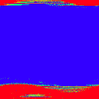
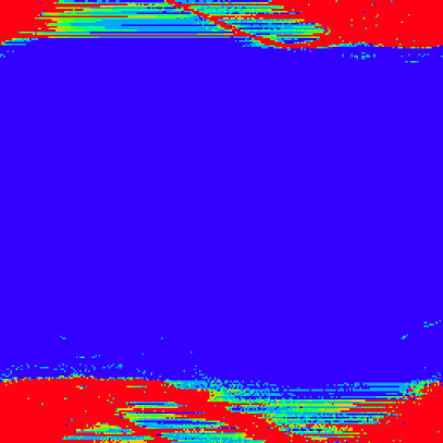
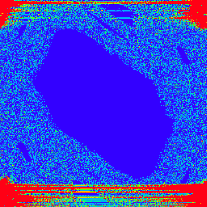
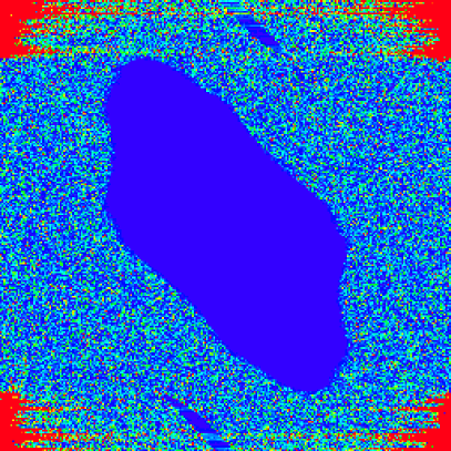
Figure 7: (Color online) Modified Husimi function (6) for the quantum kicked rotator with $K=0.5$ (top left), $K=0.9$ (top right), $K=1.5$ (bottom left), $K=2$ (bottom right). Here $T=2\pi/N$, where $N=2^{n_{q}}$, with $n_{q}=16$. The function is plotted on a lattice of $\sqrt{N}\times\sqrt{N}$ and each point is the average of $N$ points. Initial state is the same as in Fig.2 (corresponding to the initial classical distribution in Fig.1), and the function is computed after $1000$ iterations of (2). Red (gray) is maximal value, blue (black) minimal value.

In Fig.7, we show the result of performing the evolution (2) on a wave packet in $N$-dimensional Hilbert space for four different values of $K$, and then applying the partial Fourier transform. The result is an array of $\sqrt{N}\times\sqrt{N}$ points, each point representing an average over $\sim N$ neighboring values of the Wigner function. The figure shows that this transformation allows to obtain efficiently a positive phase space distribution which can be compared with the classical distributions, for example in Fig.1.

Figure 8: Scaling for the IPR $\xi$ vs $n_{q}$ for the function $H(\theta,n)$ in (7), with parameters $K=0.5$ and $T=2\pi/N$, $N=2^{n_{q}}$. Main plot: empty squares represent the IPR of $H(\theta,n)$ function , the full squares represent the IPR of the wavelet transform of the modulus of $H(\theta,n)$. The full line is $N^{0.6}$. In the inset, the ratio $R$ between IPR of $H(\theta,n)$ and wavelet transform of $|H(\theta,n)|$ is plotted for different $n_{q}$, the full line is $N^{0.6}$. Number of iterations and initial state are the same as in Fig.7.

Figure 9: Scaling for the IPR $\xi$ vs $n_{q}$ for the function $H(\theta,n)$ in (7), with parameters $K=0.9$ and $T=2\pi/N$, $N=2^{n_{q}}$. Main plot: empty squares represent the IPR of $H(\theta,n)$, the full squares represent the IPR of the wavelet transform of the modulus of $H(\theta,n)$. The full line is $N^{0.3}$, the dashed line is $N^{0.5}$. In the inset, the ratio $R$ between IPR of $H(\theta,n)$ and wavelet transform of $|H(\theta,n)|$ is plotted for different $n_{q}$, the full line is $N^{0.2}$. Number of iterations and initial state are the same as in Fig.7.

Figure 10: Scaling for the IPR $\xi$ vs $n_{q}$ for the function $H(\theta,n)$ in (7), with parameters $K=1.5$ and $T=2\pi/N$, $N=2^{n_{q}}$. Main plot: empty squares represent the IPR of $H(\theta,n)$, the full squares represent the IPR of the wavelet transform of the modulus of $H(\theta,n)$. The full line is $N^{0.2}$, the dashed line is $N^{0.7}$. In the inset, the ratio $R$ between IPR of $H(\theta,n)$ and wavelet transform of $|H(\theta,n)|$ is plotted for different $n_{q}$. Number of iterations and initial state are the same as in Fig.7.

Figure 11: Scaling for the IPR $\xi$ vs $n_{q}$ for the function $H(\theta,n)$ in (7), with parameters $K=2$ and $T=2\pi/N$, $N=2^{n_{q}}$. Main plot: empty squares represent the IPR of $H(\theta,n)$, the full squares represent the IPR of the wavelet transform of the modulus of $H(\theta,n)$. The dashed line is $N^{0.7}$. In the inset, the ratio $R$ between IPR of $H(\theta,n)$ and wavelet transform of $|H(\theta,n)|$ is plotted for different $n_{q}$, the full line is $N^{0.7}$. Number of iterations and initial state are the same as in Fig.7.

In Fig.8-11 we show the IPR of the result of this transform and of an additional wavelet transform of this function. The data show that with this modified Husimi distribution the compression of information is much better than in the case of the Wigner function.

Indeed, in all four parameter regimes considered, the IPR of the function scales as $N^{\gamma}$, with $0.5\leq\gamma\leq 0.7$. This means that the most important components of the modified Husimi distribution can be measured with $\sim N^{\gamma}$ quantum measurements. Thus on a quantum computer the whole process of evolving the wave function up to time $t$, transforming it into the modified Husimi distribution and measuring it needs $O(tN^{\gamma})$ operations. On the contrary, a classical computer will need $O(tN)$ operations for the evolution, and $O(N)$ for the modified Husimi transform (up to logarithmic factors). Thus for the system (2), computation of the modified Husimi transform is more efficient on a quantum computer (including measurement) than on a classical one. This gain would disappear if the transform had IPR $\sim N$.

As in the preceding section, one can use coarse-grained measurements in order to increase the probability. Again, this gives the integrated probability inside the cells in a number of measurements which scales with the number of cells, with the same drawbacks than in section III.

If we use amplitude amplification, the gain is even better. Amplitude amplification will need $\sqrt{N/N_{D}}$ iterations to bring the probability inside a square of size $\sqrt{N_{D}}\times\sqrt{N_{D}}$ close to one. Then according to Fig. 8-11 $N_{D}^{\gamma}$ measurements are needed, with $0.5\leq\gamma\leq 0.7$. The total number of quantum operations is therefore $O(t\sqrt{N}N_{D}^{\gamma-1/2})$. Classically, we still need $O(tN)$ operations for the evolution, and $O(\sqrt{N}\sqrt{N_{D}})$ for the transform (up to logarithmic factors). Thus for small $N_{D}$ a quadratic gain is achieved. Interestingly enough, this gain persists in the case where the IPR of the modified Husimi function is $\sim N$, even though the previous method then will not give any gain. Since the IPR cannot be larger than $N$, this means that with amplitude amplification the quantum computer is in general at least quadratically faster at evaluating part of the modified Husimi function than any classical device. If the classical algorithm to compute the evolution of the map were more complex, i.e. of order $O(tN^{k})$ with $k>1$, then in this case the quantum algorithm will be better by a factor $N^{k-1/2}$ if $N_{D}$ and $t$ are kept fixed, making the gain even larger, but still polynomial.

We also analyzed the use of the wavelet transform to compress these data and minimize the number of measurements. At this point a slight complication appears. In the previous section, individual amplitudes of the wave function in (4) were actual values of the Wigner function, so performing a quantum wavelet transform of (4) was equivalent to a wavelet transform of the Wigner function. In the case at hand, the wave function of the quantum computer is such that the modulus square of its components give the modified Husimi distribution. One can perform a quantum wavelet transform of this wave function, with real and imaginary parts for all coefficients, which gives the wavelet coefficients of a complex-valued distribution whose square is the modified Husimi distribution. It is not clear how to interpret the resulting coefficients, and anyway our data have shown that this process does not decrease the IPR (data not shown), thus making it an inefficient way of treating such data. However, Figures 8-11 show that if one take the modulus of the wave function, then the IPR of the wavelet transform of this function is quite small, scaling as $O(N^{\delta})$, with $\delta\approx 0-0.2$. So the modified Husimi function itself is well compressed by the wavelet transform. It is the phase of $H(\theta,n)$ in (7) which, although irrelevant for the Husimi functions, prevents compression by the wavelet transform. To use efficiently the wavelet transform, we therefore need to get rid of the phases, i.e. construct a wave function whose components are the moduli or moduli square of the preceding wave functions.

Such a wave function can be prepared by starting from two initial wave packets on two separate registers $|\psi_{0}\rangle\otimes|\psi_{0}^{*}\rangle$, and as in the previous section make them evolve independently to get $\hat{U}^{t}|\psi_{0}\rangle\otimes\hat{U}^{*t}|\psi_{0}^{*}\rangle$. Then a partial Fourier transform is applied independently to both registers, yielding $\sum H(\theta,n)H(\theta^{\prime},n^{\prime})^{*}|\theta\rangle|\theta^{\prime}\rangle|n\rangle|n^{\prime}\rangle$. Then amplitude amplification should be used to select the diagonal components, yielding $\sum|H(\theta,n)|^{2}|\theta\rangle|n\rangle$. These components represented a probability $N/N^{2}=1/N$ of the full original wave function, thus this process costs $O(t\sqrt{N})$ operations up to logarithmic factors. This procedure gives us a final wave function whose components are now the modified Husimi function itself, without the irrelevant phases. We can now apply the quantum wavelet transform to this wave function. Afterward, measuring the main components of the wave function should need only $O(N^{\delta})$ quantum measurements. The cost of the total procedure is therefore $O(tN^{\delta+1/2})$ quantum operations, whereas classical computation will cost $O(tN)$ operations. Obtaining the main wavelet components of this modified Husimi distribution is therefore more efficient on a quantum computer than on a classical one, albeit the gain is still polynomial.

V V. Standard images

The investigations in the previous sections show that computation of quantum phase space distributions can be more efficient on a quantum computer than on a classical device. An usually polynomial gain can be obtained for the whole process of producing the distribution and measuring its values. These phase space distributions are in effect examples of two-dimensional images. It is interesting to explore these questions of efficiency of image processing on a quantum computer in a more general setting.

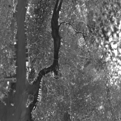
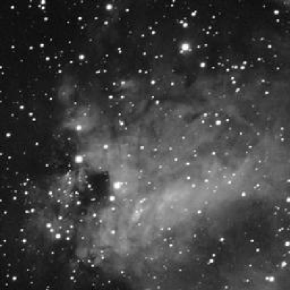
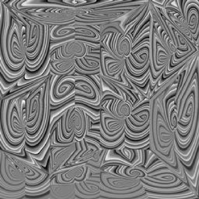
Figure 12: Images analyzed in this section. Top: girl image (left) and New York City picture (right). Bottom: galaxy image taken from NASA website (left) and a fractal picture built on the purpose of studying image compression (right).

Fig.12 shows four examples of classical images which we can use as benchmark to test different strategies of processing them. The top left image (the girl) is a standard example used in the field of classical image processing. Top right is a aerial view of New York City, bottom left an astronomical photograph, and bottom right an artificially built picture with fractal-like structures. They represent diverse types of images that can be produced and processed for various purposes. We will suppose in the following that these black and white pictures are encoded on a quantum wave function in the form $\psi=\sum_{x,y}a_{xy}|x\rangle|y\rangle$ where $x,y$ are indexes of $N^{2}$ pixels and $a_{xy}$ are the amplitudes on each pixel (positive number). Of course, contrary to the previous examples, we do not know how to produce in an efficient way such types of wave functions. We therefore concentrate on the problem of extracting information efficiently from such a wave function once it has been produced.

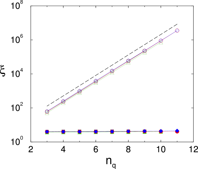
Figure 13: (Color online) Scaling for the IPR $\xi$ vs $n_{q}$ for the images with different resolutions. Full symbols: $\xi$ after wavelet transform. Empty symbols: $\xi$ for the original images. with different resolution (from 32 $\times$ 32 to 2048 $\times$ 2048). Squares refer to the girl image, circles to the New York City image, triangles to the galaxy image, and diamonds to the fractal image. The dashed line is the law $N^{2}$ with $N=2^{n_{q}}$. The original images are 8-bit gray scale images. They are encoded in the wave function from which the IPR is computed.

Fig.13 permits to analyze two of the strategies precedingly developed. The IPR of the different images are shown to scale like $N^{2}$, implying that direct measurement of all qubits will need $O(N^{2})$ measurements to get the most important components (since these components scale also like $O(N^{2})$). As in the case of the Wigner function, coarse-grained measurements are possible, and require a number of measurements proportional to the number of cells. This is more efficient, at the price of losing information on scales smaller than the cell size.

The use of amplitude amplification on a small part of the picture (polynomial in $n_{q}$) enables to bring this part to a probability close to $1$ in $O(N)$ Grover-like iteration. So if one is interested in details of the picture at a specific place predetermined, this strategy is more efficient than the direct measurement. Of course, precise efficiency of the quantum process compared to classical methods will depend on the relative complexity of the classical and quantum image production, which probably varies with the problem.

The full symbols in Fig.13 give the IPR of the wavelet transform of the image. That is, the image is encoded in a quantum wave function as previously, and a quantum wavelet transform is applied. The resulting wave function displays an IPR which grows slowly with $n_{q}$. Actually, data from Fig.13 are compatible with a polynomial growth with $n_{q}$ of the IPR. This would indicate that the wavelet transform is very efficient in compressing information from standard images. Obtaining the main components of the wavelet transform would demand polynomial number of measurements compared to an exponential one for the original image wave function. This can transfer to an exponential gain in the full process if the image can be encoded also in a polynomial number of operations in $n_{q}$.

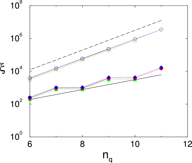
Figure 14: (Color online) Scaling for the IPR $\xi$ vs $n_{q}$ for the images with different resolutions, the tiling method (see text) is used, with tiles of size $\sim\sqrt{N}\times\sqrt{N}$ Full symbols: $\xi$ after wavelet transform. Empty symbols: $\xi$ for the original images. with different resolution (from 32 $\times$ 32 to 2048 $\times$ 2048). Squares refer to the girl image, circles to the New York City image, triangles to the galaxy image, and diamonds to the fractal image. The dashed line is the law $N^{2}$ with $N=2^{n_{q}}$, the full line is the law $N$. The original images are 8-bit gray scale images. They are encoded in the wave function and the IPR is computed from the latter.

In Fig.14, a different strategy is studied. Namely, in analogy with the MPEG standard for image compression, the image is decomposed into many tiles, and each tile is independently wavelet-transformed. This procedure is tested in the case where tiles are of size $\sqrt{N}\times\sqrt{N}$. Fig.14 shows that although the final IPR grows more quickly with $n_{q}$ than in the case of Fig.13, the IPR seems asymptotically to be smaller again than with the full image wave function. Data from Fig.14 are compatible with an IPR growing like $O(N)$, implying that the number of measurements is the square root of the one for the full wave function. This suggests a polynomial speed up with this method. We note that a similar strategy for a quantum sound treatment was discussed in lee .

Figure 15: Comparison IPR / entropy for the girl image of Fig.12. Full symbols are for IPR, empty symbols for $2^{S}$, where $S$ is the entropy. Squares and circles are for the wavelet transform, diamonds and triangles for the original image. Data for the three other images of Fig.12 give the same result.

Fig.15 enables to confirm the preceding results which use the IPR. Indeed, an alternative quantity to quantify the spreading of a wave function on a predetermined basis is the entropy. For a $N$-dimensional wave function $|\psi\rangle$ with projections on a basis $|\phi_{j}\rangle$ given by $W_{j}=|\langle\psi|\phi_{j}\rangle|^{2}$, the entropy is defined by $S=-\sum_{j}W_{j}\log_{2}W_{j}$. It takes values from $S=0$ ($\psi=\phi_{j}$ for some $j$) to $S=\log_{2}N$ ($\psi=\frac{1}{\sqrt{N}}\sum_{j}|\phi_{j}\rangle$). Both IPR and $2^{S}$ give an estimate of the number of components of the wave function. The data show that although both quantities are different, they show a similar behavior with $n_{q}$ as do their wavelet transform, confirming that the preceding results are robust.

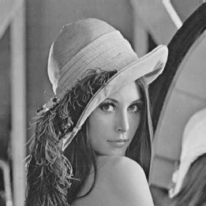
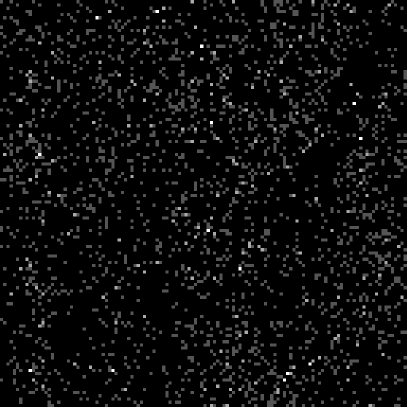
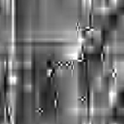
Figure 16: Image reconstruction from Monte Carlo sampling and quantum wavelet sampling. Top: exact girl image (left) and sampled with $2500$ Monte Carlo points (right). Bottom: reconstruction after sampling with $2500$ measurements in the wavelet basis after full (left) and tiled (right) wavelet transform. The images are $128\times 128$ i.e. $\sim 16000$ points in total.

The preceding discussion gives some numerical arguments suggesting that main components of the wavelet transform can be obtained more efficiently than the image itself. This gives information on the patterns present in the picture, and can be considered as an information in itself. It is also worth studying how much information about this original image is present in these main components of the wavelet transform. Fig.16 shows an attempt of reconstruction of one image from these main components only. The results displayed on this figure show that although some features are distinguishable with this technique (better than with the Monte-Carlo sampling), a lot of information from the original figure has been lost. It is possible that better results are obtained for larger system sizes, but this regime cannot be reached by our classical numerical simulations. Still, even if the largest wavelet coefficients by themselves are not enough to give a good approximation of the original image, they bring some information about it that can be obtained with a small number of measurements.

VI VI. Conclusion

In this paper, we have analyzed and numerically tested the quantum computation of Wigner and Husimi distributions for quantum systems. Two methods of computation for the Wigner function, one original to this paper, were considered. We studied different strategies to extract information from the wave function of the quantum computer, namely direct measurements, coarse-grained measurements, amplitude amplification and measure of wavelet-transformed wave function. For the Wigner function, the largest (polynomial) gain is obtained through the use of the wavelet transform, although other methods might yield a smaller gain in the chaotic regime. For the Husimi distribution, the gain is much larger, although it is still polynomial, and increases with the use of amplitude amplification and wavelet transforms. At last, the study of real images show that the wavelet transform enables to compress information and therefore to lower the number of measurements in the quantum case, although a lot of information is lost in the process.

One of the authors (M.T.) acknowledges Benjamin Lévi and Stefano Gagliano for useful discussions about classical image treatment, and for helping him in finding the high-resolution images in Fig.12. We thank the IDRIS in Orsay and CalMiP in Toulouse for access to their supercomputers. This work was supported by the EC RTN contract HPRN-CT-2000-0156 and by the project EDIQIP of the IST-FET program of the EC.

References

- (1) M. A. Nielsen and I. L. Chuang, Quantum Computation and Quantum Information (Cambridge University Press, Cambridge, 2000).
- (2) P. W. Shor, in Proceedings of the 35th Annual Symposium on the Foundations of Computer Science, edited by S. Goldwasser (IEEE Computer Society, Los Alamitos, CA, 1994), p. 124.
- (3) L. K. Grover, Phys. Rev. Lett. 79, 325 (1997).
- (4) S. Lloyd, Science 273, 1073 (1996); D. S. Abrams and S. Lloyd, Phys. Rev. Lett. 79, 2586 (1997).
- (5) R. Schack, Phys. Rev. A 57, 1634 (1998).
- (6) B. Georgeot and D. L. Shepelyansky, Phys. Rev. Lett. 86, 2890 (2001).
- (7) P. H. Song and D. L. Shepelyansky, Phys. Rev. Lett. 86, 2162 (2001).
- (8) G. Benenti, G. Casati, S. Montangero and D. L. Shepelyansky, Phys. Rev. Lett. 87, 227901 (2001).
- (9) A. A. Pomeransky and D. L. Shepelyansky, Phys. Rev. A 69, 014302 (2004).
- (10) E. Wigner Phys. Rev. 40, 749 (1932); M. V. Berry, Phil. Trans. Royal Soc. 287, 237 (1977).
- (11) S.-J. Chang and K.-J. Shi, Phys. Rev. A 34, 7 (1986).
- (12) B. Lévi, B. Georgeot and D. L. Shepelyansky, Phys. Rev. E 67, 046220 (2003).
- (13) B. Lévi and B. Georgeot, Phys. Rev. E 70, 056218 (2004).
- (14) K. M. Frahm, R. Fleckinger and D. L. Shepelyansky, Eur. Phys. J. D 29, 139 (2004).
- (15) C. Miquel, J. P. Paz, M. Saraceno, E. Knill, R. Laflamme and C. Negrevergne, Nature 418, 59 (2002).
- (16) J. P. Paz, A. J. Roncaglia and M. Saraceno, Phys. Rev. A 69, 032312 (2004).
- (17) G. Brassard and P. Høyer, in Proceedings of Fifth Israeli Symposium on Theory of Computing and Systems (IEEE Computer Society, Los Alamitos, CA, 1997) pp. 12-23; G. Brassard, P. Høyer, M. Mosca and A. Tapp, in Quantum Computation and Quantum Information: A Millenium Volume, edited by S. J. Lomonaco, Jr. and H. E. Brandt (AMS, Contemporary Mathematics Series Vol. 305, 2002).
- (18) I. Daubechies, Ten Lectures on Wavelets, CBMS-NSF Series in Applied Mathematics (SIAM, Philadelphia, 1992).
- (19) Y. Meyer, Wavelets: Algorithms and Applications (SIAM, Philadelphia, 1993).
- (20) P. Høyer, quant-ph/9702028 (1997).
- (21) A. Fijaney and C. Williams, Lecture Notes in Computer Science 1509, 10 (Springer, 1998); quant-ph/9809004.
- (22) A. Klappenecker, in Wavelet Applications in Signal and Image Processing VII, edited by M. A. Unser, A. Aldroubi, A. F. Laine, SPIE (1999), p. 703; quant-ph/9909014.
- (23) M. Terraneo and D. L. Shepelyansky, Phys. Rev. Lett. 90, 257902 (2003).
- (24) M. Kolobov, Rev. Mod. Phys. 71, 1539 (1999).
- (25) A. I. Lvovsky, H. Hansen, T. Aichele, O. Benson, J. Mlynek and S. Schiller, Phys. Rev. Lett. 87, 050402 (2001).
- (26) B. V. Chirikov, in Les Houches Lecture Series, edited by M.-J. Giannoni, A. Voros and J. Zinn-Justin, (North-Holland, Amsterdam, 1991), Vol. 52.
- (27) B. V. Chirikov, Phys. Rep. 52, 263 (1979); A. Lichtenberg and M. Lieberman, Regular and Chaotic Dynamics, (Springer, New York, 1992).
- (28) G. Casati, I. Guarneri, and D. L. Shepelyansky, IEEE Jour. of Quant. Elect. 24, 1420 (1988); P.M. Koch and K.A.H. van Leeuwen, Phys. Rep. 255, 289 (1995).
- (29) F. L. Moore, J. C. Robinson, C. F. Bharucha, B. Sundaram and M. G. Raizen, Phys. Rev. Lett. 75, 4598 (1995).
- (30) G. Benenti, G. Casati, S. Montangero and D. L. Shepelyansky, Phys. Rev. A 67, 052312 (2003).
- (31) C. Miquel, J. P. Paz and M. Saraceno Phys. Rev. A 65, 062309 (2002).
- (32) J. W. Lee, A. D. Chepelianskii and D. L. Shepelyansky, quant-ph/0309018 and in Proceedings of the SPIE conference Noise and information in nanoelectronics, sensors, and standards II edited by J.M.Smulko, Y.Blanter, M.I.Dykman, L.B.Kish, 5472, 246 (2004).