Present address: ]Institute for Quantum Information Science, University of Calgary, Calgary, AB, T2N 1N4, Canada Present address: ]Departments of Chemistry and Electrical Engineering, University of Southern California, Los Angeles, CA 90089

Entanglement Observables and Witnesses for Interacting Quantum Spin Systems

Abstract

We discuss the detection of entanglement in interacting quantum spin systems. First, thermodynamic Hamiltonian-based witnesses are computed for a general class of one-dimensional spin-$1/2$ models. Second, we introduce optimal bipartite entanglement observables. We show that a bipartite entanglement measure can generally be associated to a set of independent two-body spin observables whose expectation values can be used to witness entanglement. The number of necessary observables is ruled by the symmetries of the model. Illustrative examples are presented.

Entanglement is a striking feature of quantum mechanics, revealing the existence of non-local correlations among different parts of a quantum system. Entanglement has been recognized as an essential resource for quantum information processing Nielsen:book . This has provided strong motivation for studies probing for the presence of naturally available entanglement in interacting spin systems OConnor:01 ; Arnesen:01Gunlycke:01Wang:01 . Moreover, the realisation that entanglement can also affect macroscopic properties (such as the magnetic susceptibility) of bulk solid-state systems  Ghosh:03 ; Brukner:04a , has increased the interest in characterizations of entanglement in terms of macroscopic thermodynamical observables. An observable which can distinguish between entangled and separable states in a quantum system is called an entanglement witness Terhal:00aTerhal:02Bruss:02 . Several different methods for experimental detection of entanglement using witness operators have been proposed Bourennane:04Rahimi:04Stobinska:04 . Entanglement witnesses have recently been obtained in terms of expectation values of thermodynamical observables such as internal energy and magnetization Brukner:04 ; Toth:04 ; Bartlett:04 , and magnetic susceptibility Brukner:04a .

Our aim in this work is two-fold: first, we find an entanglement witness for a broad class of interacting spin-$1/2$ particles, thus generalizing the result of Refs. Brukner:04 ; Toth:04 ; Bartlett:04 . This is an entanglement witness for all spin-$1/2$ based solid-state quantum computing proposals, such as electron spins in quantum dots Loss:98 and P donors in Si Kane:98Vrijen:00 . While this approach is very general, its drawback is that it is sub-optimal, in the sense that it does not detect all entangled states. In contrast, in the second part of this work, we introduce the concept of an optimal bipartite entanglement observable. This allows us to construct optimal bipartite-entanglement witnesses for qubit systems. The essential idea here is to directly relate bipartite entanglement measures and the expectation value of spin observables Wang:02a .

Hamiltonian-based entanglement witnesses.— An important class of spin-based solid-state quantum computing proposals is approximately governed by diagonal exchange interactions (involving only $\sigma_{i}^{\alpha}\sigma_{j}^{\alpha}$ terms, where $\alpha\in\{x,y,z\}$ and $\sigma_{i}^{\alpha}$ is the Pauli matrix for spin $i$) Loss:98 ; Kane:98Vrijen:00 . However, spin-orbit coupling introduces off-diagonal terms into the exchange Hamiltonian Kavokin:01 . In this case previous results concerning Hamiltonian-based entanglement witnesses Toth:04 ; Brukner:04 ; Bartlett:04 do not apply, since they are restricted to the diagonal case. Here we construct an appropriately generalized entanglement witness.

The most general Hamiltonian describing $N$ nearest-neighbor coupled spin-$1/2$ particles in 1D is of the form $H=\sum_{i}\sum_{\alpha,\beta\in\{x,y,z\}}g_{i,i+1}^{\alpha\beta}\sigma_{i}^{\alpha}\sigma_{i+1}^{\beta}$, where $g_{i,i+1}^{\alpha\beta}=(g_{i,i+1}^{\beta\alpha})^{\ast}$. There are thus nine independent parameters for each pair of spins $i,i+1$. It is convenient to re-express $H$ in terms of a scalar part and symmetric and anti-symmetric parts. In addition we allow for the presence of a global external magnetic field $\mathbf{B}$: $H=-\mathbf{B}\cdot\sum_{i=1}^{N}{\bm{\sigma}}_{i}+\sum_{i=1}^{N}\sum_{\alpha=x,y,z}J_{\alpha}\sigma_{i}^{\alpha}\sigma_{i+1}^{\alpha}\\ +\sum_{i=1}^{N}\mathbf{A}\cdot({\bm{\sigma}}_{i}\times{\bm{\sigma}}_{i+1})+\sum_{i=1}^{N}(\mathbf{C}\cdot{\bm{\sigma}}_{i})(\mathbf{C}\cdot{\bm{\sigma}}_{i+1})$, where ${\bm{\sigma}}_{i}=(\sigma_{i}^{x},\sigma_{i}^{y},\sigma_{i}^{z})$, $J_{\alpha}$ are exchange coupling constants, and we assume periodic boundary conditions (${\bm{\sigma}}_{N+1}\equiv{\bm{\sigma}}_{1}$). The anisotropic term involving $\mathbf{A}$ (the Dzyaloshinskii-Moriya vector in solid-state physics) typically arises due to spin-orbit coupling; $|\mathbf{A}|/J$ has been estimated to be in the range $0.01-0.8$ in coupled quantum dots in GaAs Kavokin:01 . The vector $\mathbf{C}$ can arise also due to dipole-dipole coupling and other sources.

We now derive a thermodynamical entanglement witness for a system governed by $H$. Let $J=\max_{\alpha}\{|J_{\alpha}|\}$, $A=\max_{\alpha}\{|A_{\alpha}|\}$. Let $\langle X\rangle\equiv\mathrm{Tr}(\rho X)$, with $\rho$ the system density matrix. Let $u=\left\langle H\right\rangle/N$ be the per-spin internal energy and $\mathbf{m}=(m_{x},m_{y},m_{z})$ the magnetization vector with components $m_{\alpha}=\sum_{i=1}^{N}\left\langle\sigma_{i}^{\alpha}\right\rangle/N$. Then $H$ yields:

$$N \!\!\!\left|u+\mathbf{B}\cdot\mathbf{m}\right|\leq\left|\sum_{i=1}^{N}\sum_{\alpha=x,y,z}J_{\alpha}\left\langle\sigma_{i}^{\alpha}\sigma_{i+1}^{\alpha}\right\rangle\right|$$

$$+\left|\sum_{i=1}^{N}\left\langle\mathbf{A}\cdot({\bm{\sigma}}_{i}\times{\bm{\sigma}}_{i+1})\right\rangle\right|+\left|\sum_{i=1}^{N}\left\langle(\mathbf{C\cdot}{\bm{\sigma}}_{i})(\mathbf{C\cdot}{\bm{\sigma}}_{i+1})\right\rangle\right|.$$

Consider an arbitrary separable density matrix $\rho=\sum_{k}p_{k}\rho_{k}^{1}\otimes\rho_{k}^{2}\otimes...\otimes\rho_{k}^{N}$, where $\sum_{k}p_{k}=1$ and all $p_{k}\geq 0$. It has been shown that for such $\rho$, using the easily verified facts $\langle\sigma_{i}^{\alpha}\sigma_{i+1}^{\beta}\rangle=\left\langle\sigma_{i}^{\alpha}\right\rangle\langle\sigma_{i+1}^{\beta}\rangle$ and $\sum_{\alpha=x,y,z}\left\langle\sigma_{i}^{\alpha}\right\rangle^{2}\leq 1$, and the Cauchy-Schwarz (CS) inequality $|\sum_{i}a_{i}b_{i}|\leq(\sum_{i}a_{i}^{2}\sum_{j}b_{j}^{2})^{1/2}$, that $\left|\sum_{i=1}^{N}J_{x}\left\langle\sigma_{i}^{x}\sigma_{i+1}^{x}\right\rangle+J_{y}\left\langle\sigma_{i}^{y}\sigma_{i+1}^{y}\right\rangle+J_{z}\left\langle\sigma_{i}^{z}\sigma_{i+1}^{z}\right\rangle\right|\leq NJ$ Toth:04 ; Brukner:04 . We therefore obtain bounds for the remaining two terms. Let $x_{i}\equiv\left\langle\sigma_{i}^{x}\right\rangle$, $(xy)_{i}\equiv\left\langle\sigma_{i}^{x}\sigma_{i+1}^{y}\right\rangle$, etc. Using again the above facts and the CS inequality we have

$$| \!\!\!\sum_{i=1}^{N}\left\langle\mathbf{A}\cdot({\bm{\sigma}}_{i}\times{\bm{\sigma}}_{i+1})\right\rangle|\leq\sum_{i=1}^{N}|\left\langle\mathbf{A}\cdot({\bm{\sigma}}_{i}\times{\bm{\sigma}}_{i+1})\right\rangle|$$

$$\!\!\!\leq 2A\sum_{i=1}^{N}\left|(yz)_{i}+(zx)_{i}+(xy)_{i}\right|$$

$$\!\!\!=2A\sum_{i=1}^{N}\left|y_{i}z_{i+1}+z_{i}x_{i+1}+x_{i}y_{i+1}\right|$$

$$\!\!\!\leq 2A\sum_{i=1}^{N}(\sum_{\alpha}\left\langle\sigma_{i}^{\alpha}\right\rangle^{2})^{1/2}(\sum_{\alpha}\left\langle\sigma_{i+1}^{\alpha}\right\rangle^{2})^{1/2}\leq 2NA.$$

Note that if we assume no symmetry breaking, i.e., $\left\langle\sigma_{i}^{\alpha}\right\rangle\equiv\left\langle\sigma^{\alpha}\right\rangle$, then in fact $|\sum_{i=1}^{N}\left\langle\mathbf{A}\cdot({\bm{\sigma}}_{i}\times{\bm{\sigma}}_{i+1})\right\rangle|=0$.

We now obtain an upper bound for the third term. In the standard Bloch-sphere parametrization for the individual spin density matrices we have: $\rho=\frac{1}{2}(I+\mathbf{n}\cdot{\bm{\sigma}})$, where $|\mathbf{n}|\leq 1$. Then $\left\langle\mathbf{C}\cdot{\bm{\sigma}}\right\rangle=\mathbf{C}\cdot\mathbf{n}\leq\left|\mathbf{C}\right||\mathbf{n}|\leq\left|\mathbf{C}\right|$. Therefore,

$$| \!\!\!\sum_{i=1}^{N}\left\langle(\mathbf{C}\cdot{\bm{\sigma}}_{i})(\mathbf{C}\cdot{\bm{\sigma}}_{i+1})\right\rangle|\leq\sum_{i=1}^{N}\left|\left\langle(\mathbf{C}\cdot{\bm{\sigma}}_{i})(\mathbf{C}\cdot{\bm{\sigma}}_{i+1})\right\rangle\right|$$

$$=\sum_{i=1}^{N}\left|\left\langle\mathbf{C}\cdot{\bm{\sigma}}_{i}\right\rangle\right|\left|\left\langle\mathbf{C}\cdot{\bm{\sigma}}_{i+1}\right\rangle\right|\leq N\left|\mathbf{C}\right|^{2}.$$

These upper bounds combine to yield the entanglement witness:

$$W\equiv\left|u+\mathbf{B}\cdot\mathbf{m}\right|/(J+2A+\left|\mathbf{C}\right|^{2}).$$ (1)

The numerator consists of macroscopic, observable quantities. The denominator consists of material parameters. We have seen that separability implies $W\leq 1$. Therefore if $W>1$ the system is entangled. When $J_{\alpha}\equiv J$ and the anistropic terms in $H$ are entirely due to the spin-orbit interaction, it is possible to relate $H$ to the isotropic Heisenberg Hamiltonian via a unitary transformation Kavokin:01 ; WuLidar:03 . Applying this transformation to the examples of entangled states that are detected by $W$ in the case $\mathbf{A}=\mathbf{C}=\mathbf{0}$, found in Refs. Toth:04 ; Brukner:04 , yields examples of non-trivial entangled states detected by $W$ when $\mathbf{A},\mathbf{C}\neq\mathbf{0}$. The importance of the witness $W$ is that it is directly applicable to a wide class of spin-$1/2$ based solid-state quantum computing proposals Loss:98 ; Kane:98Vrijen:00 , where the effect of spin-orbit coupling is known to be non-negligible Kavokin:01 .

Spin-based entanglement witnesses.— Let us turn now to the construction of optimal bipartite-entanglement witnesses, based on spin observables. Consider a general two-body observable $\widehat{R}=\sum R_{\alpha\beta\gamma\delta}(ij)\left|\alpha\right\rangle_{i}\left|\beta\right\rangle_{j}\left\langle\gamma\right|_{i}\left\langle\delta\right|_{j}$, where $\{\left|\alpha\right\rangle_{i}\}$ is a basis for the Hilbert space, $i,j$ enumerate $d$ -level systems, and $\alpha,\beta,\gamma,\delta\in\{0,1,...,d-1\}$. The expectation value of $\widehat{R}$ can generally be written as WuSarandyLidar:04

$$\langle\,\widehat{R}\,\rangle=\sum_{ij}{\text{Tr}}(\mathbf{R}(ij)\mathbf{\rho}^{ij}),$$ (2)

where $\mathbf{R}(ij)$ are $d\times d$ matrices with elements $R_{\alpha\beta\gamma\delta}(ij)$ and $\rho^{ij}$ is the two-body reduced density matrix. Eq. (2) holds for any mixed state and for any $d$. Here we are especially interested in $d=2$, i.e., the qubit case. We then use the standard basis $\left\{\left|00\right\rangle,\left|01\right\rangle,\left|10\right\rangle,\left|11\right\rangle\right\}$ for any pair $(i,j)$ of spins, and denote $\rho_{11}^{ij}=\left\langle 0_{i}0_{j}\right|{\hat{\rho}}^{ij}\left|0_{i}0_{j}\right\rangle$, $\rho_{12}^{ij}=\left\langle 0_{i}0_{j}\right|{\hat{\rho}}^{ij}\left|0_{i}1_{j}\right\rangle$, etc. For an operator $\widehat{R}$ displaying a constant interaction between nearest-neighbor particles, the non-vanishing matrices $\mathbf{R}(ij)$ are given by $\mathbf{R}(i,i+1)\equiv\mathbf{R}$ $(\forall\,i)$. Moreover, if translation invariance is assumed in the system then $\rho^{i,i+1}\equiv\rho$. Hence we can rewrite Eq. (2) as

$$\langle\,\widehat{\mathcal{R}}\,\rangle={\text{Tr}}(\mathbf{R}\mathbf{\rho}),$$ (3)

where $\widehat{\mathcal{R}}=\widehat{R}/N$, with $N$ the number of nearest-neighbor pairs in the system.

A convenient bipartite entanglement measure is the negativity Vidal:02a , ranging from $0$ (no entanglement) to $1$ (maximal entanglement), defined as follows:

$$\mathcal{N}(\rho)=2\,\max(0,-\min_{\alpha}(\mu_{\alpha})),$$ (4)

where $\mu_{\alpha}$ are the eigenvalues of the partial transpose $\rho^{T_{A}}$ of the two-particle reduced density operator $\rho$, given by $\left\langle\alpha\beta\right|\rho^{T_{A}}\left|\gamma\delta\right\rangle=\left\langle\gamma\beta\right|\rho\left|\alpha\delta\right\rangle$. We denote the lowest eigenvalue of $\rho^{T_{A}}$ by $\mu_{m}$ which, for composite systems of dimensions $2\times 2$ and $2\times 3$, is non-negative if and only if the state is separable Peres:96 ; Horodecki:96 . Thus, from Eq. (4), one can see that separability implies vanishing negativity Wang:02a .

The eigenvalue $\mu_{m}$, which is the key object of our framework, is generally a non-linear function of the matrix elements of the density operator. However, let us first consider the linear case, which occurs for several interesting quantum spin systems, as will be illustrated later. In this case, we can directly relate $\mu_{m}$ to a single observable which plays the role of an entanglement witness. Indeed, assume that $\mu_{m}=\sum_{a,b=1}^{4}f_{ab}\rho_{ab}$, where $f_{ab}$ are constants. Then, defining the matrix elements of $\widehat{\mathcal{R}}$ as $R_{ab}=f_{ba}$ we obtain

$$\mu_{m}={\text{Tr}}(\mathbf{R}\rho)=\langle\,\widehat{\mathcal{R}}\,\rangle.$$ (5)

Therefore, the observable $\widehat{\mathcal{R}}$ directly detects the existence of bipartite entanglement in the system. $\langle\,\widehat{\mathcal{R}}\,\rangle<0$ implies bi-partite entanglement, while otherwise the state is separable.

Eq. (5) can also be established, formally, for those cases where $\mu_{m}$ depends non-linearly on $\rho$. Indeed, from Eq. (3) it follows that

$$\langle\,\widehat{\mathcal{R}}\,\rangle={\text{Tr}}(\mathbf{R}^{T_{A}}\mathbf{\rho}^{T_{A}})=\sum_{\alpha=1}^{4}\left\{W\mathbf{R}^{T_{A}}W^{\dagger}\right\}_{\alpha\alpha}\mu_{\alpha},$$ (6)

where the matrix $\mathbf{R}^{T_{A}}$ is defined through $\left\langle\alpha\beta\right|\mathbf{R}^{T_{A}}\left|\gamma\delta\right\rangle=\left\langle\gamma\beta\right|\mathbf{R}\left|\alpha\delta\right\rangle$, $W$ is a unitary matrix which diagonalizes $\mathbf{\rho}^{T_{A}}$ (note that $\mathbf{\rho}^{T_{A}}$ is Hermitian Peres:96 ), and the $\{\mu_{\alpha}\}$ denote the four eigenvalues of $\mathbf{\rho}^{T_{A}}$. If we choose $\widehat{\mathcal{R}}$ such that

$$W\mathbf{R}^{T_{A}}W^{\dagger}={\text{diag}}(e_{1},e_{2},e_{3},e_{4}),$$ (7)

where $e_{\alpha}=1$ for the value of $\alpha$ such that $\mu_{\alpha}=\mu_{m}$ and $e_{\alpha}=0$ for the other ones, then as desired $\langle\,\widehat{\mathcal{R}}\,\rangle=\mu_{m}$. Hence the expectation value of $\widehat{\mathcal{R}}$ can be used in general as a criterion of separability. However, in the non-linear case, if we define $\widehat{\mathcal{R}}$ through Eq. (7), $\widehat{\mathcal{R}}$ itself will be a function of the density matrix (since $W$ is). One would then need to measure a complete set of observables to find $\,\widehat{\mathcal{R}}$, which just corresponds to quantum state tomography Nielsen:book . We show below that in the presence of symmetries the number of measurements required to construct $\widehat{\mathcal{R}}$ can be drastically reduced.

XYZ spin chain in a magnetic field.— In order to provide an example of spin-based witnesses in quantum spin chains, let us consider a parametric family of spin Hamiltonians $H=\sum_{i=1}^{N}H_{i,i+1}({\bm{\theta}}_{i},{\bm{\theta}}_{i+1})$, where $H_{i,i+1}({\bm{\theta}}_{i},{\bm{\theta}}_{i+1})=U({\bm{\theta}}_{i})U({\bm{\theta}}_{i+1})H_{i,i+1}U^{\dagger}({\bm{\theta}}_{i+1})U^{\dagger}({\bm{\theta}}_{i})$, $U({\bm{\theta}}_{i})=\exp(i{\bm{\theta}}_{i}\cdot{\bm{\sigma}}_{i})$, and

$$H_{i,i+1} = J_{x}\sigma_{i}^{x}\sigma_{i+1}^{x}+J_{y}\sigma_{i}^{y}\sigma_{i+1}^{y}+J_{z}\sigma_{i}^{z}\sigma_{i+1}^{z}$$ (8)

$$+J_{xy}\sigma_{i}^{x}\sigma_{i+1}^{y}+J_{yx}\sigma_{i}^{y}\sigma_{i+1}^{x}+h\sigma_{i}^{z},$$

with periodic boundary conditions assumed, i.e. $\sigma_{N+1}^{\alpha}=\sigma_{1}^{\alpha}$. Observe that a large class of one-dimensional spin models is covered by the Hamiltonian (8). This family of Hamiltonians obeys the constraint $\left[H,\sigma_{i}^{z}\sigma_{i+1}^{z}\right]=0$ and belongs to the subalgebra $su(2)\oplus su(2)\subset su(4)$. Defining $T_{i}^{\pm}\equiv\frac{1}{2}\left(\sigma_{i}^{x}\sigma_{i+1}^{x}\pm\sigma_{i}^{y}\sigma_{i+1}^{y}\right)$, $R_{i}^{\pm}\equiv\frac{1}{2}\left(\sigma_{i}^{x}\sigma_{i+1}^{y}\pm\sigma_{i}^{y}\sigma_{i+1}^{x}\right)$, $Z_{i}^{\pm}\equiv\frac{1}{2}(\sigma_{i}^{z}\pm\sigma_{i+1}^{z})$, one of the $su(2)$ terms is generated by the set of operators $\{T_{i}^{+},R_{i}^{-},Z_{i}^{-}\}$ (respectively with coefficients $J_{x}+J_{y}$, $J_{xy}-J_{yx}$, and $h$, in $H$) and preserves the two dimensional subspace spanned by $\left\{\left|01\right\rangle,\left|10\right\rangle\right\}$. The other $su(2)$ is generated by $\{T_{i}^{-},R_{i}^{+},Z_{i}^{+}\}$ (respectively with coefficients $J_{x}-J_{y}$, $J_{xy}+J_{yx}$, and $h$, in $H$) and preserves the other two dimensional subspace spanned by $\left\{\left|00\right\rangle,\left|11\right\rangle\right\}$. The Hamiltonian $H_{i,i+1}({\bm{\theta}}_{i},{\bm{\theta}}_{i+1})$ has the same entanglement properties as $H_{i,i+1}$ since they are connected through local unitary transformations. Therefore, assuming that the initial state has the same symmetry as the Hamiltonian (no symmetry breaking), the nearest-neighbor reduced density matrix for an arbitrary mixed state reads, in the standard $\{\left|00\right\rangle,\left|01\right\rangle,\left|10\right\rangle,\left|11\right\rangle\}$ basis

$$\rho=\left[\begin{array}[]{cccc}a&0&0&y\\ 0&b&z&0\\ 0&z^{\ast}&c&0\\ y^{\ast}&0&0&d\end{array}\right].$$ (9)

Positivity of $\rho$ implies that $ad\geq|y|^{2}$ and $bc\geq|z|^{2}$, with $a,b,c,d\geq 0$. Computing the eigenvalues of $\rho^{T_{A}}$ leads to two independent possibilities for the lowest eigenvalue $\mu_{m}$:

$$\mu_{m}^{(1)} = (a+d-\sqrt{(a-d)^{2}+4\left|z\right|^{2}})/2,$$ (10)

$$\mu_{m}^{(2)} = (b+c-\sqrt{(b-c)^{2}+4\left|y\right|^{2}})/2.$$ (11)

The condition for entanglement $\mu_{m}<0$, together with positivity of $\rho$, yields the restrictions

$$\mu_{m}^{(1)} < 0\Rightarrow ad<bc,$$ (12)

$$\mu_{m}^{(2)} < 0\Rightarrow bc<ad.$$ (13)

Note that, since $\mu_{m}$ is nonlinear in the density matrix elements, the resulting witness $\widehat{\mathcal{R}}$, obtained from Eqs. (6) and (7), will be density matrix-dependent. Indeed, for $\mu_{m}=\mu_{m}^{(1)}$,

$$\widehat{\mathcal{R}} = {\rm Im}(f)R^{-}+{\rm Re}(f)T^{+}-\frac{1}{2}\frac{(a-d)}{\sqrt{(a-d)^{2}+4|z|^{2}}}Z^{+}$$ (14)

$$+ \!\!\!\frac{1}{4}\left(I\otimes I+\sigma^{z}\otimes\sigma^{z}\right),$$

where $f\equiv-z/\sqrt{(a-d)^{2}+4|z|^{2}}$, and $R^{-},T^{+},Z^{+}$ were defined above. It is seen from this result that the state-dependence can be removed if the following constraints are obeyed: $a=d$ and $z$ is either real or imaginary. These constraints are obeyed, e.g., for the isotropic Heisenberg model (see below). In this case we need to measure just one observable in order to determine the entanglement properties of the system. Analyzing the second possibility, i.e. $\mu_{m}=\mu_{m}^{(2)}$, we obtain

$$\widehat{\mathcal{R}} = -{\rm Im}(g)R^{+}+{\rm Re}(g)T^{-}-\frac{1}{2}\frac{(b-c)}{\sqrt{(b-c)^{2}+4|y|^{2}}}Z^{-}$$ (15)

$$+ \frac{1}{4}\left(I\otimes I-\sigma^{z}\otimes\sigma^{z}\right),$$

where $g\equiv-y/\sqrt{(b-c)^{2}+4|y|^{2}}$, and $R^{+},T^{-},Z^{-}$ were defined above. Similarly, $\widehat{\mathcal{R}}$ is state-independent in Eq. (15) for $b=c$ and $y$ either real or imaginary. An example of this case is given by the transverse field Ising model (see below). But even in the case of the rather general Hamiltonian (8), it is clear that instead of full-scale quantum state tomography, it suffices to measure the elements $\{a,d,z\}$ or $\{b,c,y\}$, in order to construct the witness operator $\widehat{\mathcal{R}}$.

Heisenberg model.— Let us consider the constraints $J_{x}=J_{y}=J_{z}\equiv J>0$ and $J_{xy}=J_{yx}=h=0$ in Eq. (8). Then we have the antiferromagnetic Heisenberg chain, whose Hamiltonian reads $H=J\sum_{i=1}^{N}\left(\sigma_{i}^{x}\sigma_{i+1}^{x}+\sigma_{i}^{y}\sigma_{i+1}^{y}+\sigma_{i}^{z}\sigma_{i+1}^{z}\right)$. $H$ is invariant under cyclic spin translations and has $SU(2)$ symmetry, with $H$ commuting with the total spin components $\sum_{i}\sigma_{i}^{\alpha}$, $\alpha\in\{x,y,z\}$. The elements of $\rho$ in Eq. (9) then obey further constraints, namely, $y=0$, $z=z^{\ast}<0$, $a=d=1+\langle\sigma_{i}^{z}\sigma_{i+1}^{z}\rangle$, and $b=c=1-\langle\sigma_{i}^{z}\sigma_{i+1}^{z}\rangle$, with $\langle\sigma_{i}^{z}\sigma_{i+1}^{z}\rangle\leq 0$ OConnor:01 ; Wang:02a (a). It then follows from Eq. (11) that the eigenvalue $\mu_{m}^{(2)}$ is always non-negative, whence entanglement is determined by the eigenvalue $\mu_{m}^{(1)}$, given by Eq. (10). Thus, the witness comes from the observable in Eq. (14), which becomes $\widehat{\mathcal{R}}=(\sigma_{i}^{x}\sigma_{i+1}^{x}+\sigma_{i}^{y}\sigma_{i+1}^{y}+\sigma_{i}^{z}\sigma_{i+1}^{z}+I)/4$ (for any site $i$). This yields the entanglement witness $\langle\,\widehat{\mathcal{R}}\,\rangle=\frac{1}{4}\left(u/J+1\right)$, where we have used that, due to the translation invariance and $SU(2)$ symmetry, the correlation functions satisfy the relations: $\langle\sigma_{i}^{x}\sigma_{i+1}^{x}\rangle=\langle\sigma_{i}^{y}\sigma_{i+1}^{y}\rangle=\langle\sigma_{i}^{z}\sigma_{i+1}^{z}\rangle=u/(3J)$  Wang:02a (a). Remarkably, this spin-based witness is (upto an irrelevant prefactor) precisely the Hamiltonian-based entanglement witness found in Ref. Brukner:04 (and in our generalized Hamiltonian-based result above). Since our spin-based approach is optimal for bi-partite entanglement ($\langle\,\widehat{\mathcal{R}}\,\rangle$ is essentially the negativity), this is a proof that the Hamiltonian-based witness Brukner:04 detects all bi-partite entangled states.

Transverse Field Ising model.— As a final example we analyze the ferromagnetic one-dimensional Ising chain in the presence of a transverse magnetic field. This model corresponds to taking $J_{x}=-\lambda J$ and $h=-J$ in Eq. (8), with $J>0$ and all the other couplings vanishing: $H=-J\sum_{i=1}^{N}\left(\lambda\sigma_{i}^{x}\sigma_{i+1}^{x}+\sigma_{i}^{z}\right)$. Then $y=y^{\ast}$ ($Z_{2}$ symmetry of $H$) and $b=c$ (translation symmetry of $H$) WuSarandyLidar:04 . From the analysis of the thermal correlation functions, which can be obtained analytically Barouch:71 , it can be shown that, in contrast to the Heisenberg case, entanglement is now determined by the eigenvalue $\mu_{m}^{(2)}$ in Eq. (11). From Eq. (15), our spin-based entanglement observable is then $\widehat{\mathcal{R}}=-\frac{1}{4}(\sigma_{i}^{x}\sigma_{i+1}^{x}-\sigma_{i}^{y}\sigma_{i+1}^{y}+\sigma_{i}^{z}\sigma_{i+1}^{z}-1)$ for any site $i$. The expectation value of this observable can be determined from measurements of the nearest-neighbor spin-spin correlations $\langle\sigma_{i}^{\alpha}\sigma_{i+1}^{\alpha}\rangle$. This can be done, e.g., by inelastic neutron scattering Hohenberg:74 . We note that it was shown in Ref. Brukner:04a that spin-spin correlation functions can act as entanglement witnesses in bulk solids. Our witness operator $\widehat{\mathcal{R}}$ is optimal, so that it can, moreover, yield precise macroscopic predictions. For instance, we plot in Fig. 1 the witness as a function of $\beta=1/kT$ for several values of $\lambda$, where $k$ is the Boltzmann constant and $T$ is the temperature. From this figure, we can obtain the exact critical temperature $T_{c}$ for the entanglement-separability transition. For $\lambda=1$, we have $\beta_{c}\approx 1.93$ or $kT_{c}\approx 0.51$ (in units such that $J=1$). This temperature can be compared to the value $0.41$ obtained in Ref. Toth:04 by using an energy witness. The reason for the small difference is that the energy witness of Ref. Toth:04 is derived from an entanglement bound and, despite being a good approximation, neglects some entangled states which are detected by $\widehat{\mathcal{R}}$.

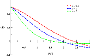
Figure 1: Witness for the transverse field Ising model. The entanglement-separability transition temperature is indicated by the intersection with the horizontal axis.

Acknowledgments.— We gratefully acknowledge financial support from CNPq-Brazil (to M.S.S.), and the Sloan Foundation, PREA and NSERC (to D.A.L.).

References

(1)
M. A. Nielsen and I. L. Chuang, Quantum Computation and Quantum
Information (Cambridge University Press, Cambridge, UK, 2000).
(2)
K. M. O’Connor and W. K. Wootters, Phys. Rev. A 63, 052302 (2001).
(3)
M. C. Arnesen, S. Bose, and V. Vedral, Phys. Rev. Lett. 87, 017901 (2001);
D. Gunlycke et al., Phys. Rev. A 64, 042302 (2001);
X. Wang, Phys. Rev. A 64, 012313 (2001); A. Saguia and
M. S. Sarandy, Phys. Rev. A 67, 012315 (2003).
(4)
S. Ghosh, T. F. Rosenbaum, G. Aeppli, and S. N. Coppersmith, Nature 425, 48
(2003).
(5)
C. Brukner, V. Vedral, and A. Zeilinger, eprint quant-ph/0410138.
(6)
B. M. Terhal, Phys. Lett. A 271, 319 (2000);
D. Bruß, J. Math. Phys. 43, 4237 (2002).
(7)
M. Bourennane et al., Phys. Rev. Lett. 92, 087902 (2004);
R. Rahimi et al., eprint quant-ph/0405175;
M. Stobinska and K. Wódkiewicz, Phys. Rev. A 71, 032304 (2005).
(8)
C. Brukner and V. Vedral, eprint quant-ph/0406040.
(9)
G. Toth, Phys. Rev. A 71, 010301(R) (2005) .
(10)
M. R. Dowling, A. C. Doherty, and S. D. Bartlett, Phys. Rev. A 70, 062113 (2004).
(11)
D. Loss and D. P. DiVincenzo, Phys. Rev. A 57, 120 (1998).
(12)
B. E. Kane, Nature 393, 133 (1998);
R. Vrijen et al., Phys. Rev. A 62, 012306 (2000).
(13)
We note that conceptually related studies established a connection between concurrence
and correlation functions: (a) X. Wang and P. Zanardi, Phys. Lett. A 301, 1 (2002);
(b) U. Glaser, H. Buttner, and H. Fehske, Phys. Rev. A 68, 032318 (2003).
(14)
K. V. Kavokin, Phys. Rev. B 64, 075305 (2001);
K. V. Kavokin, Phys. Rev. B 69, 075302 (2004).
(15)
L.-A. Wu and D. A. Lidar, Phys. Rev. Lett. 91, 097904 (2003).
(16)
L.-A. Wu, M. S. Sarandy, and D. A. Lidar, Phys. Rev. Lett. 93, 250404 (2004).
(17)
G. Vidal and R. F. Werner, Phys. Rev. A 65, 032314 (2002).
(18)
A. Peres, Phys. Rev. Lett. 77, 1413 (1996).
(19)
M. Horodecki, P. Horodecki, and R. Horodecki, Phys. Lett. A 223, 1
(1996).
(20)
E. Barouch and B. M. McCoy, Phys. Rev. A 3, 786 (1971).
(21)
P. C. Hohenberg and W. F. Brinkman, Phys. Rev. B 10, 128131 (1974).