Scalar and vector modulation instabilities induced by vacuum fluctuations in fibers:
numerical study

Abstract

We study scalar and vector modulation instabilities induced by the vacuum fluctuations in birefringent optical fibers. To this end, stochastic coupled nonlinear Schrödinger equations are derived. The stochastic model is equivalent to the quantum field operators equations and allow for dispersion, nonlinearity, and arbitrary level of birefringence. Numerical integration of the stochastic equations is compared to analytical formulas in the case of scalar modulation instability and non depleted pump approximation. The effect of classical noise and its competition with vacuum fluctuations for inducing modulation instability is also addressed.

I Introduction

In the early 1980s single-mode silica optical fibers were recognized as a privileged medium for experiments in quantum optics because they exhibit a well defined transverse mode and very low losses. The Kerr nonlinearity of silica has been used to produce non classical states of light. Squeezed state production in fibers was pioneered by Levenson et al. Levenson et al. (1985a, b) in 1985. Since then a large number of squeezing experiments have been performed with cw-light or short optical pulses (for a review see Sizmann and Leuchs (1999)).

More recently, Fiorentino et al. demonstrated that optical fibers may also be used to produce twin-photons pairs Fiorentino et al. (2002). This new kind of twin-photon source is well suited for fiber-optic quantum communication and quantum cryptography networks. In contrast with the traditional twin-photon sources, based on the $\chi^{(2)}$ down-conversion process, it avoids large coupling losses occurring when the pairs are launched into long distance communication fibers. The physical process used in Fiorentino et al. (2002) to generate twin-photon pairs is a four-wave mixing (FWM) phase-matched by the interplay of the optical Kerr effect and the chromatic dispersion, called (scalar) modulation instability (MI). This process can be basically understood as the destruction of two pump photons at frequency $\omega_{0}$ and the creation of Stokes (red-shifted) and anti-Stokes (blue-shifted) photons at frequencies $\omega_{s}$ and $\omega_{a}$ satisfying the energy conservation relation $2\omega_{0}=\omega_{s}+\omega_{a}$. In the time domain, the beating of the pump, signal and idler waves produces a fast modulation of the pump envelope.

MI is a spontaneous phenomena which can be described in the framework of classical nonlinear optics Agrawal (1995). In this classical framework, one usually considers that MI is induced by some incoherent noise initially present on the pump wave. Twin-photon pair production requires however a very low input noise power to be efficient (otherwise the twin-photons are buried in the background photon noise). Such a regime is dominated by vacuum fluctuations and requires a quantized field theory to be described properly. A small-perturbation approach of this problem Potasek and Yurke (1987) (non depleted pump approximation) shows that vacuum fluctuations can induce the MI even in the absence of any classical input noise. This is an ideal situation for twin-photon pairs production, but it never occurs in a real life experiment. In practice, classical input noise and vacuum fluctuations compete for inducing MI.

Understanding the dynamical development of MI from a quantum point of view is an important issue for the design of fiber-optics twin-photon pairs sources. We present an unified approach to this problem based on the stochastic nonlinear Schrödinger equations (SNLSE) Carter et al. (1987); Drummond and Carter (1987); Kennedy and Wright (1988); Kennedy and Wabnitz (1988); Kennedy (1991); Drummond and Corney (2001). This formalism is equivalent to quantum-field Heisenberg equations but has two main advantages. First, it is very suitable for numerical simulations of complex situations where classical noise and vacuum fluctuations act together. Second the correspondence principle of quantum physics, i.e. the transition from quantum to classical world, looks very natural in the SNLSE formalism.

The MI observed in standard non-birefringent single-mode silica fibers is often referred to as scalar modulation instability (S-MI) because polarization of light plays no role in this process. In birefringent fibers different kinds of MI may appear because of the interplay of nonlinearity, chromatic dispersion and birefringence. This case will be referred as vector modulation instability (V-MI). Twin-photon pairs sources based on V-MI have not been demonstrated yet, in contrast with S-MI based sources Fiorentino et al. (2002). In this article, we will however address both issues because we recognize that V-MI twin-photon pairs sources could be more practicable than S-MI based ones. The theoretical and computational tools that we developed apply to all kind of MI, including the low-birefringence, high-birefringence and scalar limits.

This article is divided into four sections, beginning with the present introduction. The second section consists of a review of the approach based on a perturbation analysis around the steady state solution. This is the simplest method of approaching the problem of MI. It allows us to set the stage for the more sophisticated approach we then develop and to make contact with earlier work in the field. Then in Sec. III we exhibit the SNLSE for scalar and vector MI. Contrary to the approach of Sec. II these equations are not based on a perturbation analysis and are valid in the strongly non linear regime. They describe both MI originating from classical noise and from vacuum fluctuations (quantum noise). The SNLSE we obtain generalize the earlier results of Carter et al. (1987); Drummond and Carter (1987); Kennedy and Wright (1988); Kennedy and Wabnitz (1988); Kennedy (1991). In particular the SNLSE we obtain does not require the birefringence to be either small or large as in earlier work Kennedy and Wabnitz (1988); Kennedy (1991), but are valid for all values of the birefringence. For the interested reader we present a self contained derivation of these equations in the Appendix. In Sec. IV we use the split-step Fourier method to integrate the SNLSE derived in Sec. III, and illustrate our algorithm on the cases of scalar MI and of vector MI both for weak, intermediate, and strong birefringence. In order to interpret the results of the numerical integration it is essential to introduce the notion of mode. This allows us to compare the numerical results and the analytical solutions derived from perturbation theory. We also compare in detail the characteristics of MI induced by classical noise and by quantum noise. In a companion article Amans et al. (2004) we shall show that our numerical results are in very good quantitative agreement with experimental results.

II Scalar modulation instability: perturbation analysis

As pointed out in the introduction several kind of MI can occur in optical fibers. From a general point of view, MI occurs when the continuous wave (steady-state) propagation is unstable. The most straightforward way to get some insight on how the MI develops is to perform a small-perturbation analysis of the steady-state. However this method has limitations: it cannot address the strongly non linear regime and simple analytical formulas cannot be always obtained by this method.

In this section we illustrate the perturbation method in the case of S-MI, which is the simplest. S-MI occurs in isotropic fibers in the anomalous dispersion regime. In what follows we will review the most important aspects of this approach, focussing on the comparison between the classical and quantum descriptions, and on the limitations of this approach. In Sec. IV, we will compare the analytical formulas for S-MI derived from the perturbation analysis to numerical results from the SNLSE derived in Sec. III. The discussion of MI in birefringent fibers is also postponed to Sec III and Sec. IV.

II.1 Classical description

In an isotropic single-mode fiber, the electric field may be written

$$\mathbf{E}(\mathbf{r},t)=F(x,y)A(z,t)\exp[i\beta_{0}z-\omega_{0}t]\mathbf{\hat{x}}+\mathrm{c.c.}$$ (1)

where $\mathbf{\hat{x}}$ is a unit vector orthogonal to the fiber axis ($z$-axis), $\omega_{0}$ the carrier angular frequency and $\beta_{0}=\beta(\omega_{0})$ the associated propagation wave number (modal propagation constant). $F(x,y)$ stands for the mode profile function and $A(z,t)$ for the field envelope. The field is supposed to be polarized linearly. This is not restrictive because of the isotropy assumption. The complex envelope $A$ evolves according to the nonlinear Shrödinger equation (NLSE) that can be established from Maxwell’s electromagnetic theory Agrawal (1995). If the envelope is normalized in such way that $|A(z,t)|^{2}$ is equal to the instantaneous power flowing through the plane $z=\text{constant}$ at time $t$, the NLSE is obtained in the following form:

$$\frac{\partial A}{\partial z}+\frac{1}{v_{g}}\frac{\partial A}{\partial t}=-i\frac{\beta_{2}}{2}\frac{\partial^{2}A}{\partial t^{2}}+i\gamma|A|^{2}A.$$ (2)

Here $v_{g}=(d\beta/d\omega)^{-1}$ is the group velocity of the wave, $\beta_{2}=d^{2}\beta/d\omega^{2}$ the group-velocity dispersion (GVD) parameter and $\gamma$ is fiber nonlinearity parameter defined as

$$\gamma=\frac{3\omega_{0}\chi_{xxxx}}{4\epsilon_{0}n_{0}^{2}c^{2}A_{\text{eff}}}$$ (3)

where $n_{0}$ is the fiber mean linear index of refraction, $A_{\text{eff}}$ the mode effective area and $\chi_{xxxx}$ is the diagonal element of the fiber $\chi^{(3)}$ nonlinearity tensor.

S-MI is observed when a continuous wave (cw) or a quasi-cw optical pulse is launched into the fiber. In the cw-case, when an optical power $P_{0}$ at frequency $\omega_{0}$ in injected, a first order perturbation analysis of Eq. (2) shows that the cw steady-state solution $A_{st}(z)=\sqrt{P_{0}}\exp{(i\gamma P_{0}z)}$ becomes instable in the anomalous dispersion regime ($\beta_{2}<0$). The instability manifests itself by a parametric gain at frequencies $\omega_{0}\pm\Omega$ with $0<\Omega<2\sqrt{\gamma P_{0}/|\beta_{2}|}$. The maximal gain $g=2\gamma P_{0}L$ occurs for $\Omega=\sqrt{2\gamma P_{0}/|\beta_{2}|}\equiv\Omega_{\text{max}}$ Agrawal (1995). Noise at these frequencies is strongly amplified. As a result, the optical spectrum at the fiber output exhibits two sidebands at frequencies $\omega_{0}\pm\Omega_{\text{max}}$. This analysis supposes that the pump power remains constant (undepleted pump approximation) and a cw regime. However, numerical simulations of Eq. (2) show that the above formula also hold for quasi-cw (for instance nanosecond) optical pulses (see Sec. IV).

Sideband generation can be interpreted as a FWM process phase-matched by the interplay of dispersion and Kerr nonlinearity. From this point of view, the MI process can be seen as the destruction of two pump photons at frequency $\omega_{0}$ followed by the creation of Stokes and anti-Stokes photons at frequencies $\omega_{s}=\omega_{0}-\Omega_{\text{max}}$ and $\omega_{a}=\omega_{0}+\Omega_{\text{max}}$ respectively. In the cw-case and non depleted pump approximation, the output power spectral density at frequencies $\omega_{s}$ and $\omega_{a}$ can be computed using analytical formulas Stolen and Bjorkholm (1982) for given initial conditions. These formulas also hold for quasi-cw pulses provided one replace Stokes and anti-Stokes power spectral densities by the number $n_{s}$ and $n_{a}$ of Stokes and anti-Stokes photons located in the same temporal mode as the pump wave (see Sec. IV.2 for a detailed analysis of this issue). For example, assuming an incoherent initial noise, one finds

$$n_{s}(L) = n_{s}(0)\cosh^{2}(\gamma P_{0}L)+n_{a}(0)\sinh^{2}(\gamma P_{0}L),\phantom{MM}$$ (4a)

$$n_{a}(L) = n_{a}(0)\cosh^{2}(\gamma P_{0}L)+n_{s}(0)\sinh^{2}(\gamma P_{0}L),\phantom{MM}$$ (4b)

where $L$ is the propagation distance. These equations show that classical incoherent noise is amplified exponentially with gain $g=2\gamma P_{0}L$.

Noise induced S-MI was first demonstrated experimentally by Tai et al. in 1986 Tai et al. (1986a). This experiment confirmed two main predictions of the classical theory: the amplification of Stokes and anti-Stokes photons and the power-dependence of their frequency shift. However the classical theory of S-MI only holds when the initial number of noise photons is high or in a stimulated regime when a coherent probe pulse at Stokes or anti-Stokes frequency is injected together with the pump pulse Tai et al. (1986b). Eqs. (4) are unable to explain ab nihilo generation of Stokes and anti-Stokes twin-photons reported in Fiorentino et al. (2002). Neither are they valid when the mean photon numbers $n_{s}(0)$ and $n_{a}(0)$ are of the order of one or lower. In this regime vacuum fluctuations play a central role and field quantization is required.

II.2 Quantum description

To take into account vacuum fluctuations, fields must be quantized. The quantum counterpart of the NLSE (2) is known as the quantum nonlinear Shrödinger equation (QNLSE) Kennedy and Wright (1988); Lai and Haus (1989); Wright (1991); Haus (2000); Korolkova and Leuchs (2001):

$$\frac{\partial\hat{A}}{\partial z}+\frac{1}{v_{g}}\frac{\partial\hat{A}}{\partial t}=-i\frac{\beta_{2}}{2}\frac{\partial^{2}\hat{A}}{\partial t^{2}}+i\gamma\hat{A}^{\dagger}\hat{A}\hat{A},$$ (5)

where $\hat{A}$ is the quantum operator corresponding to the field envelope and $\hat{A}^{\dagger}$ its hermitic conjugated. $\hat{A}$ and $\hat{A}^{\dagger}$ satisfy the bosonic equal-space commutation rule:

$$\left[\hat{A}(z,t),\hat{A}^{\dagger}(z,t^{\prime})\right]=\hbar\omega_{0}\delta(t-t^{\prime}).$$ (6)

The normalization constant $\hbar\omega_{0}$ stems from the normalization chosen for the field envelope. In the quantum propagation theory, the expectation value of the optical power flowing through the plane $z=\text{constant}$ at time $t$ is given by $\langle\hat{A}^{\dagger}(z,t)\hat{A}(z,t)\rangle$. In a one dimensional system, space and time play a symmetrical role. The dynamics can be described either in terms of spatial wave-packet evolution (evolution picture) or in terms of temporal wave-packet propagation (propagation picture). The first picture is the must common in quantum field theory and leads to equal-time commutation rules between the envelope fields $\hat{A}$ and $\hat{A}^{\dagger}$. In this section however, we chose to work in the propagation picture (which is usual in nonlinear optics) in order to get a closer correspondence between quantum (5) and classical (2) equations. In this case equal-space commutation rules (6) must be imposed to $\hat{A}$ and $\hat{A}^{\dagger}$ Blow et al. (1990). (In contrast, the evolution picture is used in the Appendix A to derive the stochastic equations of Sec. III.)

In the cw regime, the basics of the quantum theory of S-MI can be understood by performing a first-order perturbation analysis of the steady state solution of Eq. (5). Because the pump field contains a large number of photons one can treat it as a classical coherent wave. Using this approximation the steady-state solution is just the classical one: $A_{st}(z)=\sqrt{P_{0}}\exp{(i\gamma P_{0}z)}$. The disturbed field can be written as:

$$\hat{A}(z,t)=A_{st}(z)+\hat{a}(z,t).$$ (7)

The disturbance operator $\hat{a}(z,t)$ is defined by Eq. (7). It satisfies the same commutation rule as $\hat{A}(z,t)$:$\left[\hat{a}(z,t),\hat{a}^{\dagger}(z,t^{\prime})\right]=\hbar\omega_{0}\delta(t-t^{\prime})$. Injecting the ansatz (7) into Eq. (5) one obtains a propagation equation for the disturbance $\hat{a}(z,t)$. Supposing that the disturbance is small (non depleted pump approximation) this equation can be linearized and solved analytically in the Fourier domain Potasek and Yurke (1987).

Using this method one finds that the quantum and classical theory predict the same frequency dependence of the parametric gain. In contrast the quantum and classical theory differ in that they do not predict the same growth law for Stokes and anti-Stokes photon numbers. One easily finds that the quantum counterparts of Eqs. (4) are

$$n_{s}(L) = n_{s}(0)\cosh^{2}(\gamma P_{0}L)$$ (8a)

$$+[n_{a}(0)+1]\sinh^{2}(\gamma P_{0}L),$$

$$n_{a}(L) = n_{a}(0)\cosh^{2}(\gamma P_{0}L)$$ (8b)

$$+[n_{s}(0)+1]\sinh^{2}(\gamma P_{0}L),$$

where $n_{s}$ and $n_{a}$ stand now for the expectation values of the photon number operators: $n_{i}=\langle\hat{n}_{i}\rangle$, $i=s,a$. These equations show that S-MI can be observed even in absence of any classical input noise. Setting $n_{s}(0)=n_{a}(0)=0$ in Eqs. (8) gives the number of Stokes and anti-Stokes photons produced by the sole action of vacuum fluctuations:

$$n_{s}(L)=n_{a}(L)=\sinh^{2}(\gamma P_{0}L).$$ (9)

Eqs. (8) hold only for perfectly phase-matched photons at frequencies $\omega_{s}$ and $\omega_{a}$ and uncorrelated initial noise but can be easily generalized to get round these restrictions.

Although Eqs. (8) and (9) give a good insight into the physics of vacuum-fluctuations induced S-MI and photon pairs generation, they are not suitable for quantitative predictions in the pulsed regime. This is because the effective value of the pump power $P_{0}$ depends on pump pulse shape, duration, and spectral width. Furthermore the energy spectral density of Stokes and anti-Stokes waves deduced from (9) is highly dependent on the precise definition of modes. This will be discussed in Sec. IV.2. In the next sections we will show how to get around these difficulties by introducing the SNLSE and solving it numerically.

III Scalar and vector modulation
instabilities: Stochastic equations

One can go beyond the perturbation analysis of S-MI by solving the QNLSE (5) numerically. Such a plan could seem cumbersome because Eq. (5) is a field-operator equation. The problem can be bypassed by converting the operator equation (5) into c-number equations. This can be performed by choosing a representation for the electromagnetic field. In this article, we will use the positive $P$-representation ($P^{(+)}$) introduced by Drummond and Gardiner Drummond and Gardiner (1980). The c-number equations obtained in this way are not standard deterministic partial derivative equations but stochastic (Langevin-type) ones.

Using the $P^{(+)}$ representation, it can be shown Drummond and Carter (1987); Carter et al. (1987); Kennedy and Wright (1988) that the QNLSE (5) is equivalent to the following set of stochastic equations:

$$\frac{\partial A}{\partial z}+\frac{1}{v_{g}}\frac{\partial A}{\partial t} = -i\frac{\beta_{2}}{2}\frac{\partial^{2}A}{\partial t^{2}}+i\gamma[A^{\dagger}(z,t)A(z,t)]A(z,t)+\sqrt{i\gamma\hbar\omega_{0}}~{}\zeta_{1}(z,t)~{}A(z,t),$$ (10a)

$$\frac{\partial A^{\dagger}}{\partial z}+\frac{1}{v_{g}}\frac{\partial A^{\dagger}}{\partial t} = +i\frac{\beta_{2}}{2}\frac{\partial^{2}A^{\dagger}}{\partial t^{2}}-i\gamma[A^{\dagger}(z,t)A(z,t)]A^{\dagger}(z,t)+\sqrt{-i\gamma\hbar\omega_{0}}~{}\zeta_{2}(z,t)~{}A^{\dagger}(z,t).\phantom{MM}$$ (10b)

Eqs. (10a) and (10b) look like the classical NLSE (2) and its complex conjugated, except for the last terms which accounts for vacuum fluctuations. These last terms contains two independent zero-mean Gaussian white noise random fields $\zeta_{1}(z,t)$ and $\zeta_{2}(z,t)$ characterized by the following second order moments:

$$\langle\zeta_{k}(z,t)\zeta_{l}(z^{\prime},t^{\prime})\rangle=\delta_{kl}\delta(z-z^{\prime})\delta(t-t^{\prime}),$$ (11)

with $(k,l)\in\{1,2\}^{2}$. Because the random fields $\zeta_{1}$ and $\zeta_{2}$ are not complex conjugated of each other, the envelope fields $A$ and $A^{\dagger}$ are only complex conjugated ”in mean” and have to be treated as different mathematical objects.

Eqs. (10) can be solved on a computer. The numerical methods used for this task will be briefly explained in Sec. IV.1. Note that solving Eqs. (10) gives a single realization of the stochastic process. In order to calculate the expectation value of a quantum observable, a statistical average on many realizations is required. Thus one generates a large number of realizations $(A_{[n]}(z,t),A^{\dagger}_{[n]}(z,t))$, $n=1,\ldots,N$. In order to calculate the expectation value of a quantum observable one then carries out a statistical average over the many realizations. For example, the expectation value of the energy spectral density of a pulse is given by:

$$S_{E}(z,\Omega)={1\over N}\sum_{n=1}^{N}\tilde{A}_{[n]}^{\dagger}(z,\Omega)\tilde{A}_{[n]}(z,\Omega),$$ (12)

where $\tilde{X}(z,\Omega)=\int_{-\infty}^{\infty}X(z,t)~{}e^{i\Omega t}~{}dt$ designates the Fourier transform of the field $X(z,t)$ and $\Omega$ is the detuning from the pump angular frequency $\omega_{0}$.

In practice, a few realizations are enough when the number of photons per mode is high. However in a regime dominated by vacuum fluctuations hundreds of realizations are typically required to get precise values. A comparison between Stokes and anti-Stokes photon production predicted by the SNLSE (10) and the analytical formulas (8) will be presented in sections IV.2 and IV.3.

The V-MI occurs in birefringent fibers. These fibers are characterized by different propagation constants $\beta_{0x}$ and $\beta_{0y}$ and different group velocities $v_{gx}$ and $v_{gy}$ for the $x$- and $y$-axis polarized modes. The numerical study of vacuum fluctuations induced V-MI requires an extension of Eqs. (10) that takes into account the phase mismatch parameter $\Delta\beta_{0}=\beta_{0x}-\beta_{0y}$ as well as the group-velocity mismatch $\Delta\beta_{1}=1/v_{gx}-1/v_{gy}$. Such extensions have been established in earlier works for the low-birefringence Kennedy and Wabnitz (1988) and the hight-birefringence Kennedy (1991) limits. We generalized these results for an arbitrary level of birefringence and obtained the following stochastic coupled nonlinear Schrödinger equations:

$$\frac{\partial A_{x}}{\partial z}+\frac{1}{v_{gx}}\frac{\partial A_{x}}{\partial t} = -i\frac{\beta_{2}}{2}\frac{\partial^{2}A_{x}}{\partial t^{2}}+i\gamma\left[A_{x}^{\dagger}A_{x}+(1-B)A_{y}^{\dagger}A_{y}\right]A_{x}+i\gamma B(A_{y})^{2}A_{x}^{\dagger}e^{-2i\Delta\beta_{0}z}$$ (13a)

$$+\sqrt{i\gamma\hbar\omega_{0}}\left[\zeta_{1}A_{x}+\sqrt{B}\zeta_{3}A_{y}e^{-i\Delta\beta_{0}z}\right],$$

$$\frac{\partial A_{x}^{\dagger}}{\partial z}+\frac{1}{v_{gx}}\frac{\partial A_{x}^{\dagger}}{\partial t} = +i\frac{\beta_{2}}{2}\frac{\partial^{2}A_{x}^{\dagger}}{\partial t^{2}}-i\gamma\left[A_{x}^{\dagger}A_{x}+(1-B)A_{y}^{\dagger}A_{y}\right]A_{x}^{\dagger}-i\gamma B(A_{y}^{\dagger})^{2}A_{x}e^{+2i\Delta\beta_{0}z}$$ (13b)

$$+\sqrt{-i\gamma\hbar\omega_{0}}\left[\zeta_{2}A_{x}^{\dagger}+\sqrt{B}\zeta_{4}A_{y}^{\dagger}e^{+i\Delta\beta_{0}z}\right],$$

$$\frac{\partial A_{y}}{\partial z}+\frac{1}{v_{gy}}\frac{\partial A_{y}}{\partial t} = -i\frac{\beta_{2}}{2}\frac{\partial^{2}A_{y}}{\partial t^{2}}+i\gamma\left[A_{y}^{\dagger}A_{y}+(1-B)A_{x}^{\dagger}A_{x}\right]A_{y}+i\gamma B(A_{x})^{2}A_{y}^{\dagger}e^{+2i\Delta\beta_{0}z}$$ (13c)

$$+\sqrt{i\gamma\hbar\omega_{0}}\left[\zeta_{1}A_{y}-\sqrt{B}\zeta_{3}A_{x}e^{+i\Delta\beta_{0}z}\right],$$

$$\frac{\partial A_{y}^{\dagger}}{\partial z}+\frac{1}{v_{gy}}\frac{\partial A_{y}^{\dagger}}{\partial t} = +i\frac{\beta_{2}}{2}\frac{\partial^{2}A_{y}^{\dagger}}{\partial t^{2}}-i\gamma\left[A_{y}^{\dagger}A_{y}+(1-B)A_{x}^{\dagger}A_{x}\right]A_{y}^{\dagger}-i\gamma B(A_{x}^{\dagger})^{2}A_{y}e^{-2i\Delta\beta_{0}z}$$ (13d)

$$+\sqrt{-i\gamma\hbar\omega_{0}}\left[\zeta_{2}A_{y}^{\dagger}-\sqrt{B}\zeta_{4}A_{x}^{\dagger}e^{-i\Delta\beta_{0}z}\right],$$

where $(A_{x},A_{x}^{\dagger})$ and $(A_{y},A_{y}^{\dagger})$ are stochastic envelope fields associated to the $x$- and $y$-axis modes respectively, and $B=\chi_{xyyx}/\chi_{xxxx}$ is a parameter that measures the strength of the nonlinear coupling between the $x$ and $y$ components. Its value lies between 0 and 1 and depends on the nonlinearity mechanism. For silica fiber, we can set $B=1/3$ because the Kerr non linearity has principally an electronic origin. Four independent gaussian random fields $\zeta_{k}(z,t)$ are needed to reproduce the effect of vacuum fluctuations. They are characterized by the second order moments (11), as in the scalar case, with $(k,l)\in\{1,2,3,4\}^{2}$. The demonstration of this set of equations is outlined in the Appendix A.

Note that, in contrast to the scalar case, a perturbation analysis does not lead to simple analytical formulas for vacuum-fluctuations induced V-MI. For this reason Eqs. (13) constitute a valuable theoretical tool.

IV Numerical integration of the SNLSE

IV.1 Sample Spectra

We have developed a method for integrating numerically the SNLSE in the case where the pump is represented by a pulse of finite duration. Our method is based on the split-step Fourier (SSF) method Agrawal (1995). We have had to generalize the method in two ways. First of all the stochastic noise is modeled by including a noise term at each propagation step. Second in the case of the V-MI we must alternate not only between the time and Fourier domain, but also between the linear and circular polarization basis. Switching from time to Fourier domain is the basics of the SSF method: it permits to handle the time-derivatives in a simple way. Similarly, it turns out that, whereas the terms with time-derivatives are easier to handle in the linear polarization basis, the $\gamma$-dependent terms are better managed in the circular polarization basis.

The quantum noise in the SNLSE (13) contains four independent real zero-mean Gaussian white noise functions $\zeta_{k}(z,t)$ characterized by Eq. (11). In the numerical method, time and space are discretized with respective discretization steps $\tau$ and $h$. So each family of noise functions $\zeta_{k}(z,t)$ becomes a finite number of random variables $\zeta_{k}[i_{z},i_{t}]$ chosen according to a zero-mean Gaussian law of variance $\frac{1}{h\tau}$. The variance value is imposed by the normalization condition (11). The matrixes $\zeta_{k}[i_{z},i_{t}]$ ($k=1,...,4$) define the stochastic path of each realization. In contrast, when we will study the effect of classical noise we will add it once, at the beginning of the pulse propagation, to the spectral distribution of the signal $\tilde{A}(0,\Omega)$.

As we have previously indicated only the expectation values of observables have a physical meaning in the stochastic equations. From a numerical point of view this means that one must average the calculated quantities over several realizations of the stochastic path, and/or the classical input noise. Usually, averaging over a hundred of realizations gives an uncertainty on the numerical results less than $1$ dB in the non-zero gain frequency-range. Finally we note that including the stochastic terms do not increase significantly the numerical complexity of a single realization.

Some sample spectra obtained using our algorithm are presented in Fig. 1 in the cases of S-MI (Fig. 1a), low birefringence V-MI (Fig. 1b), and high birefringence V-MI (Fig. 1c). The energy spectral density is plotted versus the frequency detuning from the pump. The physical parameters used in these simulations are listed in Table 1. In every simulation, the pump wave has been supposed to be an unchirped linearly polarized Gaussian pulse with peak power $P_{0}$ and full-width-half-maximum duration $T_{\text{FWHM}}$. No classical noise has been added, and an average over 50 realizations of the stochastic process has been performed.

		Fig. 1a	Fig. 1b	Fig. 1c
$\lambda_{0}$	[nm]	1550	1550	1064
$\beta_{2}$	[ps2km-1]	-17	+60	+30
$\gamma$	[W-1km-1]	2	2	2
$T_{\text{FWHM}}$	[ns]	1	0.1	0.2
$P_{0}$	[W]	2	400	300
$\Delta\beta_{0}$	[m-1]	0	2.09	628.31
$\Delta\beta_{1}$	[fs m-1]	0	1.72	354.91
$\theta$	[degree]	0	0	45

Table 1: Simulation parameters for Fig. 1a-c.

The frequency detuning of the side bands agrees with linear perturbation theory. (In order to make the comparison easier we have indicated in Fig. 1a-c the angular frequency shifts $\Omega_{\text{max}}$ at which maximum gain is expected on the basis of the linear perturbation theory.)

Moreover the SNLSE predict quantitatively the effect of vacuum fluctuations on the evolution of the energy spectral density of the electromagnetic field. In Sec. IV.2 we will show that this evolution is also in very good agreement with linear perturbation theory when the number of Stokes and anti-Stokes photons generated is small enough. When the side bands are well-developed, the perturbation theory fails to predict correct values of $S_{E}$. In contrast, the SNLSE algorithm still gives accurate results. In this limit numerical results can be easily confronted to experimental data. In Amans et al. (2004), we report an experiment on high birefringence spontaneous V-MI in the anomalous dispersion regime that shows that the theoretical spectra from the SNLSE model tally with the experimental ones.

It is interesting to note that the curves of Fig. 1a look more noisy than those of Fig. 1b although we have performed the same number of stochastic realizations in both cases. This is because the number of realizations needed to achieve a given precision on the expectation value of a quantum operator is a function of the relative value of the spatial step $h$ and the typical distance over which the nonlinear effects act; both are different in the simulations of Fig. 1a and Fig. 1b. In practice, the smaller the spatial step, the fewer the number of realizations needed to achieve a given precision on expectation values. In Fig. 1, 50 realizations are enough to estimate $S_{E}$ with an accuracy of about $1.5$ dB.

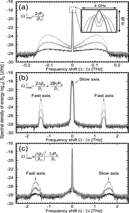
Figure 1: MI spectra for various birefringence regime. Simulation parameters are listed in Tab. 1. (a) Spontaneous S-MI in perfectly isotropic fiber in the anomalous dispersion regime. Black, dark gray and light gray curves correspond to a propagation length $L$ = 500, 1000, 1500 m, respectively. The inset exhibits the pump spectral broadening due to the self-phase-modulation (SPM) effect. (b) Spontaneous V-MI in a slightly birefringent fiber in the normal dispersion regime. The pump is polarized along the slow axis, Stokes and anti-Stokes photons appear on the orthogonal axis. Black, dark gray and light gray curves correspond to a propagation length $L$ = 16, 24, 32 m, respectively. (c) Spontaneous V-MI in a strongly birefringent fiber in the normal dispersion regime. The pump polarization axis makes an angle of 45 degrees with the slow axis. Stokes (anti-Stokes) photons appear on the slow (fast) axis. Black, dark gray and light gray curves correspond to a propagation length $L$ = 10, 20, 30 m, respectively.

We also point out that the noise level visible at non phase-matched frequencies has no physical meaning. It can be lowered by averaging over a higher number of realizations. However, the number of realizations needed to achieve an accurate estimation of $S_{E}$ in the non phase-matched part of the spectrum is usually very high. When tractable, a linear perturbation analysis will be less time-consuming.

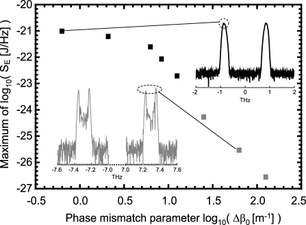
Figure 2: The figure illustrates the effect of an increasing birefringence on the weak-birefringence V-MI phenomenology. The parameters of the simulations are: $\lambda_{0}=1550$ nm, $\beta_{2}=$ 60 ps² km^-1, $\gamma=2$ W^-1 km^-1, $T_{\text{FWHM}}=100$ ps, $P_{0}=$ 400 W, and $L=$  40 m. The pump wave is polarized along the slow axis. The fiber beat-length was varied from 10 m to 5 cm. The values of $\Delta\beta_{0}$ and $\Delta\beta_{1}$ where deduced from Eq. (14). The plot shows the maximum value of $S_{E}$ in the side bands as a function of $\Delta\beta_{0}$. Black squares (gray squares) correspond to a single (double) peak structure (see the text).

Because our algorithm permits to investigate intermediate birefringence, we have also studied the effect of group velocity mismatch on the transition from low to high birefringence limits. To our knowledge, this transition has never been fully investigated before. Fig. 2 shows the results of simulations with the same parameters as in Fig. 1b except that the propagation length has been set to $L=40$ m and that the fiber beat length $L_{B}$ was varied from 10 m to 5 cm. The value of the maximal energy spectral density $S_{E}$ in the side bands is plotted versus the phase mismatch parameter. By lowering $L_{B}$, we increase the value of the phase mismatch $\Delta\beta_{0}$ and the group-velocity mismatch $\Delta\beta_{1}$ according to the relations

$$\Delta\beta_{0}=\frac{2\pi}{L_{B}},\quad\Delta\beta_{1}=\frac{\lambda_{0}}{cL_{B}},$$ (14)

where $c$ is the vacuum speed of light. When the birefringence increases, the side bands move away from the pump spectrum and their amplitude decreases. Subsequently the side bands acquire a double peak structure (see Fig. 2). This behavior is due to the walk-off of the produced Stokes and anti-Stokes photons. One easily shows that $1/v_{ga}-1/v_{gs}=\sqrt{8\beta_{2}\Delta\beta_{0}}$, where $v_{gs}$ and $v_{ga}$ are the Stokes and anti-Stokes photons group velocities, respectively. Applying this formula to our simulation and taking $\Delta\beta_{0}=10$ m^-1, one sees that the Stokes and anti-Stokes photons have walked 87.6 ps away while their FWHM duration is 100 ps. Stokes and anti-Stokes walk-off limits the coherent exponential amplification of quantum noise. The typical length scale over which the side bands growth takes place is given by $T_{\text{FWHM}}/\sqrt{8\beta_{2}\Delta\beta_{0}}$. We point out that this analysis also hold for a cw-pump: The coherent amplification of the side bands stops when the walk-off of Stokes and anti-Stokes photons exceeds the coherence length of the pump. However, in the cw-case, Stokes and anti-Stokes photons generated in the first coherence length act as an input noise that will be amplified in the following coherence length. The process is reproduced as many times as the number of coherence lengths in the propagation distance. One usually argues Memyuk (1987); Agrawal (1995) that the weak birefringence phenomenology disappears because the coherent-coupling terms in Eqs. (13) (those containing the factor $\exp[\pm(2)i\Delta\beta_{0}z]$) average to zero when $\Delta\beta_{0}$ is high. This statement is equivalent to saying that $\Omega_{\text{max}}$ tends to infinity. Our analysis shows however that walk-off has an even stronger effect.

Until now we have not yet demonstrated that modeling vacuum-fluctuations induced MI using SNLSE predicts the correct values of $S_{E}$. In subsections IV.2 we compare the absolute values of the energy spectral density at the maximum gain obtained using our program and the linear perturbation analysis. Having clarified in this way the interpretation of the results of our numerical simulations we turn to a detailed comparison of the effect of classical and quantum noises. That is we compare the effects of classical noise in the initial conditions and the quantum noise added at each step of the integration.

IV.2 Comparing numerical integration and linear perturbation theory

In our numerical simulations we have taken the pump laser to be a Gaussian pulse without chirp. Its instantaneous power and energy spectral density can be written

$$P(t) = P_{0}\exp(-\frac{t^{2}}{2\sigma_{t}^{2}}),$$ (15a)

$$S_{E}(\Omega) = \frac{P_{0}}{2\sigma_{\omega}^{2}}\exp(-\frac{\Omega^{2}}{2\sigma_{\omega}^{2}})$$ (15b)

with $\sigma_{t}\sigma_{\omega}=\frac{1}{2}$. The numerical integration of the SNLSE provides us with the spectral density of energy $S_{E}(L,\Omega)$ at the end of the fiber, see Eq. (12). On the other hand the linear perturbation theory is based on small perturbation analysis around a continuous monochromatic pump. We would like to compare quantitatively the predictions of these two approaches.

For definiteness we carry out this comparison in the case of scalar MI. We shall focus our investigation on the intensity of the sidebands at the peak of the MI gain ($\Omega=\Omega_{\text{max}}$) in the two approaches when we modify the propagation length and as we modify the duration $\sigma_{t}$ of the pulse.

The linear perturbation theory is based on a continuous monochromatic pump. For this reason the theory predicts a rate of photon production per unit time. This suggests that if one takes the pump to be a pulse localized in time, the number of photons produced should be proportional to the pulse duration, all other parameters being kept constant. Simulations based on SNLSE confirm this phenomenology. This is illustrated in Fig. 3a, where the energy spectral density at $\Omega_{\text{max}}$ is plotted as a function of $\gamma P_{0}L$ for three different pulse durations. Note however that the above argument is valid for square pulses but is not very satisfactory for Gaussian ones. A better understanding of the origin of this scaling can be obtained by making appeal to the notion of mode and of Heisenberg box.

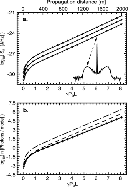
Figure 3: Values of the number of photons created at the maximum gain frequency obtained by integrating numerically the SNLSE as a function of propagation length $L$. In order to keep the maximum gain frequency constant we have kept the peak power $P_{0}$ constant in each figure. The horizontal axis is given in dimensionless units of $\gamma P_{0}L$ where $P_{0}$ is either the power of the continuous pump wave in the linear approximation, or the peak power of the Gaussian pump pulse. The top panel is plotted in the density of energy representation whereas the bottom panel is plotted in the number of photons-per-mode representation using the rescaling of Eq. (16). In both panels, the up-triangles, the circles and the down-triangles correspond to FWHM durations respectively equal to 4 ns, 1 ns and 0.25 ns. Note that these three curves coincide perfectly in panel (b), thereby showing the relevance of the rescaling (16). In the bottom panel, the dash-dotted line results from the analytic solution Eq. (9). The dashed line corresponds to Eq. (9) convoluted with the pump shape then rescaled according to Eq. (16), see the text. All other parameters are identical to those used in Fig. 1a.

In order to introduce the notion of mode, recall that a temporal signal can be represented by a distribution in the time-frequency plane. But because of the time-frequency uncertainty relations, a point in this plane has no physical meaning. This problem is well known in signal processing where one usually thinks in terms of local time-frequency decompositions, using windowed Fourier transforms (WFT) or wavelet transforms Mallat (1999). Such a local time-frequency decomposition allows one to decompose a signal into orthogonal local functions, called modes. These can be depicted as surface elements in the time-frequency plane. Fourier-transform limited pulses, such as our pump pulse (15), are represented by Gaussian distributions on the time-frequency plane, called the Wigner-Ville distributions. This distribution is very similar to the Wigner distribution used in quantum optics to represent a quantum state of light. In particular two different Fourier-limited Gaussian pulses sufficiently different in time or central frequency can be considered as quasi-orthogonal modes. A set of quasi non overlapping Gaussian Wigner-Ville distributions can be taken as a base for the time-frequency decomposition of the field. One can visualize this modal base by imagining that the time-frequency plane is paved with adjacent elementary surface elements, called Heisenberg boxes, roughly representing the area of Gaussian quasi non overlapping Wigner-Ville distributions. The precise area of the Heisenberg boxes is a matter of taste depending on how strong orthogonality is required. A usual convention is to take this area equal to $\sigma_{t}\times\sigma_{\omega}=1/2$.

This set of (quasi) mode is convenient for our problem because, during the pulse propagation in the fiber, the uncertainty on the creation time of a photon is defined by the variance $\sigma_{t}^{2}$ of the pump pulse, and implies an uncertainty on its frequency defined by the variance $\sigma_{\omega}^{2}$. More precisely, in the case of S-MI, the pump pulse (15) produces photons that occupy single Heisenberg boxes located at the same time as the pump but at angular frequencies $\omega_{0}\pm\Omega$ ($0<\Omega<\sqrt{2}\Omega_{\text{max}}$). Formulas (8) and (9) of Sec. II.2 thus give the number of photons created in these Stokes and anti-Stokes modes.

Our numerical simulations provide us with the spectral distribution of energy $S_{E}$. Hence we need to reexpress this as the number $n$ of photons produced per mode of duration $\sigma_{t}$ and spectral width $\sigma_{\omega}$:

$$n(\Omega)=\frac{S_{E}(\Omega)}{\hbar\omega_{0}}\times\sigma_{\omega}=\frac{S_{E}(\Omega)}{\hbar\omega_{0}}\frac{\sqrt{2\ln 2}}{T_{\text{FWMH}}}.$$ (16)

Fig. 3b shows the effect of scaling the spectra according to Eq. (16). When expressed in terms of number of photons per modes the three curves of Fig. 3a (corresponding to three different pump durations) come down to a single one in Fig. 3b (continuous line). This shows that the notion of mode helps in interpreting the results of the numerical integration. The number of produced photons does not depend of the pump duration: The pump duration just alters their time-frequency characteristics. The dash-dotted curve in Fig. 3b corresponds to a direct application of Eq. (9). A discrepancy with the simulations based on the SNLSE can be noted. It is simply due to the fact that our choice of size of Heisenberg boxes, hence the normalization factor in Eq. (16), is somewhat arbitrary. By taking the Heisenberg boxes a bit bigger, one can put the continuous and dash-dotted curves of Fig 3b in superposition. In the rest of the text, however, we maintain the normalization relation Eq. (16) for clarity.

There is another way to compare the results of SNLSE simulations to the linear perturbation theory that avoids the concept of modes. One first computes the power spectral density given by the quantum perturbation analysis on a monochromatic pump wave. Then one convolutes this with the Gaussian spectral distribution of the real pump pulse. This procedure gives a good approximation of the energy spectral density generated by the Gaussian pump. The dashed curve of Fig. 3b corresponds to the peak energy spectral density computed by this method and rescaled according to Eq. (16) in order to be independent of the pulse duration. The agreement with the continuous curve is now much better. The origin of the small difference in slope in the exponential amplification regime still remains unclear. It may be due to the self-phase-modulation broadening of the pump spectrum, which is not taken into account by the linear perturbation analysis.

As a conclusion we obtain a good quantitative agreement between the simulation based on SNLSE and the linear perturbation analysis. We have also shown that the only physical quantity that can be rigorously predicted by the quantum nonlinear propagation theory is the energy spectral density and that the concept of mode, although very useful, must be handled with care. Especially formulas like (8) and/or (9) may only be used as a rough approximation tool because there is no objective way to define a time-frequency mode.

IV.3 Classical versus Quantum Noise

From Figs. 3 it is clear that the spontaneous MI growth can be divided into two different stages. So long as the number of particles created by mode is less than one ($n<1$), one is in a quantum regime dominated by vacuum fluctuations. In contrast, for $n$ above 1 the modulation instability is amplified exponentially and quantum effects become negligible.

We now investigate the transition between the quantum and classical regimes in presence of some classical noise. We have chosen to model this noise by modifying the initial conditions and adding a white noise to the amplitude of the pump pulse in the Fourier domain. For definiteness and simplicity, we continue to focus on scalar modulation instability.

The classical initial noise $\widetilde{N}(\Omega)$ was chosen according to two criteria: (i) the noise must correspond to a random fluctuation of the pump amplitude in the time domain and (ii) the statistic of $\widetilde{N}(\Omega)$ (for each frequency) must lead to a spectral density of energy $\langle\widetilde{N}(\Omega)\widetilde{N}^{\ast}(\Omega)\rangle$ constant as a function of the frequency. Several noise definitions can meet these criteria. We have chosen to study two particular cases : the pure spectral phase noise

$$\widetilde{N}_{\phi}(\Omega)=\widetilde{A}\exp(i\pi\zeta(\Omega)),$$ (17)

and the Gaussian noise

$$\widetilde{N}_{\text{G}}(\Omega)=\frac{\widetilde{A}}{\sqrt{2}}\times(\zeta_{1}(\Omega)+i\zeta_{2}(\Omega)),$$ (18)

where $\widetilde{A}$ is a real constant and $\zeta_{j}(\Omega)$ are independent real zero-mean Gaussian white noise random fields. In our simulations $\zeta_{j}(\Omega)$ where discretized and replaced with random quantities $\zeta_{j}[i_{\omega}]$ (one for each discretized frequency) drawn according a zero-mean Gaussian law of variance 1. We have compared S-MI spectra averaged over 50 realizations, obtained from both classical noises (with quantum noise set to zero). Both noises lead to equivalent results. The difference between the spectra is lower than 0.3 dB on the full spectral span, which is less than the residual averaging noise (See Fig.1a), and therefore negligible. Hereafter, the classical noise is set according to Eq. (17). It corresponds to a white flux of photons without any phase correlations between each frequency component.

In Fig. 4 we compare the peak intensity of side bands in the case of vacuum-fluctuations induced MI and the (unphysical) case of MI induced by the classical noise alone. In the quantum regime where the number of particles per mode is small the two approaches differ strongly whereas in the exponential amplification regime they give similar results, although different classical noise levels give rise to different final number of photons.

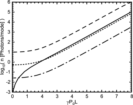
Figure 4: Comparison between a MI growing from quantum noise (solid line) and from purely classical noise. The number of photons in the Stokes and anti-Stokes modes is plotted as a function of the propagation length (expressed in dimensionless units $\gamma P_{0}L$). The input noises in the classical situation correspond to the following amount of photons per mode: (i) $1/40$ (dash-dotted line), (ii) $1/2$ (dotted line), and (iii) 10 (dashed line). The simulation parameters are those of Fig. 1a.

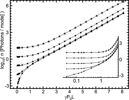
Figure 5: Simulated values of the number of photons in the Stokes and anti-Stokes modes in the realistic case when MI grows from both quantum and classical noise. The classical noise intensities are defined in order to correspond to an amount of photons per GHz: (i) 0.1 (circles), (ii) 1 (up-triangles), (iii) 10 (down-triangles), and (iv) 100 (stars). The squares correspond to a purely quantum noise. The simulation parameters are those of Fig. 1a. The inset is a zoom corresponding to the the lowest $\gamma P_{0}L$-parameters. It is drawn in a logarithmic-scale.

The simulations of Fig. 5 take into account both classical and quantum noises. They illustrate the realistic situation when both noises compete for producing modulation instability. If the order of magnitude of the classical noise is such that there is less than one photon per mode, the quantum noise dominates and the curve is (except for very small values of the gain) indistinguishable from the case where there is no classical noise. On the other hand if the number of noise photons per mode is much larger than one, the classical noise dominates and the intensity of the sidebands is indistinguishable from purely classical situations depicted in Fig. 4. These numerical results are consistent with Eqs. (8), in which the term 1 represents the contribution of the vacuum fluctuation. If $n_{s}$ or $n_{a}$ are higher than 1, Eqs. (8) tend to Eqs. (4) corresponding to the classical description.

In summary we have shown that if one considers only the peak intensity of the sidebands, the quantum origin of the instability can only be seen in the regime where the number of photons per mode (produced or initially present) is small whereas when the number of photons per mode is large the effect of vacuum fluctuations is indistinguishable from that of classical noise. Good quantitative agreement between the two approaches in the exponential amplification regime is obtained when the number of noise photons is $1/2$ per mode. Note that other quantum effects, such as two mode squeezing, may be present in the regime where many photons are produced per mode, but exhibiting them requires looking at correlations between the two sidebands.

IV.4 Using classical noise to compute the instabilities induced by vacuum fluctuations

We can now discuss the well-known trick which consists in introducing a half photon per mode into a classical simulation (then removing it) to simulate the spontaneous effects. To see how this works we compare Eqs. (4) which describe the MI induced by classical noise and Eq. (9) which is derived from the quantum theory and gives the number of photons produced per mode by the action of vacuum fluctuations alone. Now, if we introduce the same amount of Stokes and anti-Stokes noise photons $n_{0}$ in Eqs. (4) we find:

$$\frac{n_{a}^{Cl}}{2n_{0}}-\frac{1}{2}=\frac{n_{s}^{Cl}}{2n_{0}}-\frac{1}{2}=\sinh^{2}(\gamma P_{0}L)=n_{a}^{Qu}=n_{s}^{Qu},$$ (19)

where $Cl$ and $Qu$ denote respectively the classical approach and the quantum approach. Taking $n_{0}=\frac{1}{2}$, Eq. (19) shows the agreement between the quantum predictions (right hand side) and the classical predictions (left hand side). Note that $n_{0}$ can be any real value (except for 0), hence the spontaneous growth of the number of photons per mode can be simulated with any number of initial classical photons if the pump depletion is neglected.

We have compared, using numerical integration, the direct quantum approach based on the SNLSE (without classical noise) and the classical approach in which one first integrates the NLSE with some initial classical noise then rescales the spectra according to the left side of Eq. (19). The discrepancy between both approaches is measured by the following ratio in dB scale:

$$\eta=10\log_{10}\left(\frac{n^{Qu}}{\frac{n^{Cl}}{2n_{0}}-\frac{1}{2}}\right),$$ (20)

Applying Eq. (20) to the data reported in Fig. 4, one founds that for $\gamma P_{0}L$ higher than 0.2, $\eta$ is constant for any classical noise amplitude: $\eta$=1.9 dB $\pm$0.3 dB. Note that both noise definitions Eq. (17) and Eq. (18) lead to the same $\eta$. Moreover this results may be extended to $\gamma P_{0}L$ lower than 0.2 by increasing the number of realizations. The origin of non-zero value of $\eta$ may come from the mode definition used in Eq. (16). Indeed the numerical integration of SNLSE gives the physical spectral density of energy $S_{E}$ whereas the calculus trick — left hand side of Eq. (19) — leads to values interpreted as a number of photons per mode which must be rescaled to give $S_{E}$.

In summary, in the case of pump pulses of finite duration, a full quantum treatment based on the SNLSE leads to a direct quantitative prediction whereas the calculus trick only gives a good approximation whose accuracy is dependent of the modes definition.

V Conclusion

We generalized to an arbitrary level of birefringence the stochastic nonlinear Schrödinger equations describing the propagation of pulses through a nonlinear $\chi^{(3)}$ medium with linear birefringence and group-velocity dispersion, and developed numerical routines to compute them. Because these stochastic equations are equivalent to quantum field operator equations, we used them to compute spontaneous (or vacuum-fluctuations induced) modulation instability spectra in various birefringence regimes, including weak, high but also intermediate birefringence which has not been studied so far. In particular we showed that the decline of the number of photons generated by the weak-birefringence V-MI when the birefringence increases, is attributable to the increase of the walk-off between Stokes and anti-Stokes photons, although the weak-birefringence V-MI gain remains constant. We then investigated the absolute values of the energy spectral density at the maximum gain in the case of scalar modulation instabilities induced by vacuum fluctuations. We obtained good quantitative agreement between the simulation based on SNLSE and the linear perturbation analysis. Then we have carried out a detailed comparison of the effect of classical and quantum noise and shown that the quantum origin of the instability can only be seen in the regime where the number of photons per mode produced or initially present is small. Finally we note that the quantum nonlinear propagation theory predicts the energy spectral density and that the concept of mode, although very useful, must be handled with care. The present work forms the basis for numerical and experimental investigation of vacuum-fluctuations induced V-MI in regimes which have been little investigated so far, and we hope to report on this in the near future Amans et al. (2004).

Although we have not developed this aspect in this article the stochastic equations can also be used to computed intensity correlations between side bands and predict special quantum effects like squeezing. For this reason the stochastic equations (13) are a valuable tool for computing quantum effects in birefringent nonlinear $\chi^{(3)}$ media, especially optical fibers. The stochastic model may also be adapted to include Raman and Brillouin effects (see Drummond and Corney (2001) for the scalar case). Higher order dispersion effects can also be included in a straightforward way.

*

Appendix A Stochastic coupled nonlinear Schrödinger equations

In order to derive the SNLSE (13), we will proceed in three stages. First, we will establish the interaction Hamiltonian that governs field evolution in a lossless, dispersive, and birefringent fiber. We will only present an heuristic derivation of this Hamiltonian and put the emphasis on appropriate approximations. A rigorous derivation requires a discussion of electromagnetic field quantization in material media Hillery and Mlodinow (1984); Drummond (1990); Blow et al. (1990); Drummond and Corney (2001), which is outside the scope of this article. Second, we will use this Hamiltonian to find the Liouville equation describing the evolution of the density operator of the field and convert it into a Fokker-Planck equation using the $P^{(+)}$-representation. Finally, we will establish the connection between the Fokker-Planck equation and the stochastic equations (13).

A.1 Linear and Nonlinear Hamiltonians

In a dispersive birefringent medium the positive-frequency part of the $s$-polarized electric field component ($s=x,y$) can be decomposed on monochromatic modes in the following way Blow et al. (1990):

$$\hat{E}^{(+)}_{s}(\mathbf{r})=i\int d\beta\left(\frac{\hbar~{}\omega_{s}(\beta)~{}v_{gs}(\beta)}{4\pi\epsilon_{0}n_{s}(\beta)cA}\right)^{\frac{1}{2}}\hat{a}_{s}(\beta)F(x,y)e^{i\beta z}.$$ (21)

Eq. (21) can be seen as defining $\hat{a}_{s}(\beta)$. The operators $\hat{a}_{s}(\beta)$ and its hermitic conjugated $\hat{a}_{s}^{\dagger}(\beta)$ are, respectively, the annihilation and creation operators for a $s$-polarized photon propagating in the fiber with a propagation constant $\beta$ and having an angular frequency $\omega_{s}(\beta)$. According to the canonical quantization, they satisfy the commutation rule

$$[\hat{a}(\beta),\hat{a}^{\dagger}(\beta^{\prime})]=\delta(\beta-\beta^{\prime}).$$ (22)

In Eq. (21), $n_{s}(\beta)$ and $v_{gs}(\beta)$ are respectively the linear index of refraction and group velocity corresponding to the $s$-polarized monochromatic mode with frequency $\omega_{s}(\beta)$, and

$$A=\int\int|F(x,y)|^{2}dxdy.$$ (23)

The operator representing the $s$-polarized electric field component is given by

$$\hat{E}_{s}(\mathbf{r})=\hat{E}^{(+)}_{s}(\mathbf{r})+\hat{E}^{(-)}_{s}(\mathbf{r}),$$ (24)

where $\hat{E}^{(-)}_{s}(\mathbf{r})=[\hat{E}^{(+)}_{s}(\mathbf{r})]^{\dagger}$ is the negative-frequency part of $\hat{E}_{s}(\mathbf{r})$.

The total Hamiltonian $\hat{H}_{T}$ representing the sum of the vacuum electromagnetic energy and the dielectric energy stored in the fiber can be decomposed in a linear part $\hat{H}_{L}$ and a nonlinear one $\hat{H}_{NL}$.

The linear part,

$$\hat{H}_{L}=\int d\beta\sum_{s=x,y}\hbar\omega_{s}(\beta)\hat{a}_{s}^{\dagger}(\beta)\hat{a}_{s}(\beta),$$ (25)

takes into account the free-field energy and the energy stored into the dielectric through linear interactions, including the effects of linear dispersion and linear birefringence through the dispersion relations $\omega_{s}=\omega_{s}(\beta)$.

If the field bandwidth is narrow compared to the central angular frequency $\omega_{0}$, dispersion can be neglected in the $\chi^{(3)}$ interactions and the nonlinear part of the Hamiltonian can be written

$$\hat{H}_{NL}=-\frac{1}{4}\epsilon_{0}d\int d^{3}r\sum_{ijkl}\chi_{ijkl}E_{i}^{(-)}E_{l}^{(-)}E_{j}^{(+)}E_{k}^{(+)},$$ (26)

where $\chi_{ijkl}$ stands for $\chi_{ijkl}(\omega_{0};\omega_{0},\omega_{0},-\omega_{0})$. This simplified Hamiltonian only takes into account the Kerr effect, which is the dominant one for quasi-monochromatic fields. Since the medium is supposed lossless, the $\chi^{(3)}$ tensor has the full permutation symmetry Boyd (1992). The degeneracy factor $d=6$ takes this symmetry into account, by counting the number of way to permute the frequency arguments and the indexes of the $\chi^{(3)}$ tensor. A further useful approximation is to consider that the $\chi^{(3)}$ process is isotropic Svirko and Zheludev (1998); Boyd (1992):

$$\chi_{ijkl}=\chi_{xxyy}\delta_{ij}\delta_{kl}+\chi_{xyxy}\delta_{ik}\delta_{jl}+\chi_{xyyx}\delta_{il}\delta_{jk}.$$

Since the field bandwidth is supposed narrow, the permutation symmetry also requires that $\chi_{xxyy}=\chi_{xyxy}$:

$$\chi_{ijkl}=\chi_{xyxy}(\delta_{ij}\delta_{kl}+\delta_{ik}\delta_{jl})+\chi_{xyyx}\delta_{il}\delta_{jk}.$$ (27)

Using Eq. (27), the nonlinear Hamiltonian becomes

$$\hat{H}_{NL}=-\frac{3}{2}\epsilon_{0}\chi_{xxxx}\int d^{3}r \bigg{(} \sum_{s}\hat{E}_{s}^{(-)}\hat{E}_{s}^{(-)}\hat{E}_{s}^{(+)}\hat{E}_{s}^{(+)}+(1-B)\sum_{s\neq s^{\prime}}\hat{E}_{s}^{(-)}\hat{E}_{s^{\prime}}^{(-)}\hat{E}_{s}^{(+)}\hat{E}_{s^{\prime}}^{(+)}$$ (28)

$$+B\sum_{s\neq s^{\prime}}\hat{E}_{s}^{(-)}\hat{E}_{s}^{(-)}\hat{E}_{s^{\prime}}^{(+)}\hat{E}_{s^{\prime}}^{(+)}\bigg{)},$$

where we defined $B=\chi_{xyyx}/\chi_{xxxx}$, and factored out $\chi_{xxxx}=2\chi_{xyxy}+\chi_{xyyx}$.

Another consequence of the narrow-bandwidth assumption is that the square-rooted bracket in Eq. (21) can be taken out of the integral and one can write

$$\hat{E}^{(+)}_{s}(\mathbf{r})\approx i\left(\frac{\hbar\omega_{0}v_{gs0}}{2\epsilon_{0}~{}n_{s0}~{}c~{}A}\right)^{1/2}F(x,y)\hat{\psi}_{s}(z,t)e^{i(\beta_{s0}z-\omega_{0}t)},$$ (29)

where

$$\hat{\psi}_{s}(z,t)=\frac{e^{i(\omega_{0}t-\beta_{s0}z)}}{\sqrt{2\pi}}\int d\beta_{s}~{}\hat{a}_{s}(\beta_{s})~{}e^{i\beta_{s}z}.$$ (30)

In Eqs. (29) and (30), $n_{s0}$, $v_{gs0}$, and $\beta_{s0}$ stand respectively for the index of refraction, the group-velocity, and the propagation constant at frequency $\omega_{0}$ on the $s$-axis. The operator $\hat{\psi}$ is an envelope operator because fast oscillations in space and time have factored out. This implies that $\hat{\psi}$ is explicitly time-dependent in the Schrodinger picture. The operator $\hat{\psi}_{s}^{\dagger}\hat{\psi}_{s}dz$ represents the number of $s$-polarized photons in $[z,z+dz]$. One can easily check that

$$[\hat{\psi}_{s}(z,t),\hat{\psi}_{s^{\prime}}^{\dagger}(z^{\prime},t)]=\delta_{ss^{\prime}}\delta(z-z^{\prime}).$$ (31)

Using Eq. (29), $\hat{H}_{NL}$ takes the following simple form:

$$\hat{H}_{NL}=-\frac{\hbar}{2}\Theta\int \Big{[} \Big{(}\hat{\psi}_{x}^{\dagger}\hat{\psi}_{x}^{\dagger}\hat{\psi}_{x}\hat{\psi}_{x}+\hat{\psi}_{y}^{\dagger}\hat{\psi}_{y}^{\dagger}\hat{\psi}_{y}\hat{\psi}_{y}\Big{)}+2(1-B)\hat{\psi}_{x}^{\dagger}\hat{\psi}_{y}^{\dagger}\hat{\psi}_{x}\hat{\psi}_{y}$$ (32)

$$+B\Big{(}(\hat{\psi}_{x}^{\dagger})^{2}\hat{\psi}_{y}^{2}e^{2i\Delta\beta_{0}z}+(\hat{\psi}_{y}^{\dagger})^{2}\hat{\psi}_{x}^{2}e^{-2i\Delta\beta_{0}z}\Big{)}\Big{]}dz,$$

where

$$\Theta=\frac{3\hbar\omega_{0}^{2}v_{g0}^{2}\chi_{xxxx}}{4\epsilon_{0}n_{0}^{2}c^{2}A_{\text{eff}}},\quad A_{\text{eff}}=\frac{A^{2}}{\int\int|F(x,y)|^{4}dx~{}dy}.$$ (33)

Let’s note that we have set $n_{0}\equiv n_{x0}\approx n_{y0}$ and $v_{g0}\equiv v_{gx0}\approx v_{gy0}$. The linear Hamiltonian $\hat{H}_{L}$ can also be expressed in function of the operators $(\hat{\psi}_{s},\hat{\psi}^{\dagger}_{s})$, $s=x,y$, by developing $\omega_{s}(\beta)$ in a Taylor expansion around $\beta_{s0}$ up to the second order,

$$\omega_{s}(\beta)=\omega_{0}+\omega^{\prime}_{s}(\beta-\beta_{s0})+\frac{\omega^{\prime\prime}_{s}}{2}(\beta-\beta_{s0})^{2}+...,$$ (34)

where $\omega^{\prime}_{s}=\frac{d\omega_{s}}{d\beta}|_{\beta_{0}}=v_{gs0}$ and $\omega^{\prime\prime}_{s}=\frac{d^{2}\omega_{s}}{d\beta^{2}}|_{\beta_{0}}$. Using Eq. (34) and inverting Eq. (30), one finds that $\hat{H}_{L}=\hat{U}+\hat{H}^{\prime}_{L}$, where

$$\hat{U}=\hbar\omega_{0}\sum_{s=x,y}\int\hat{\psi}_{s}^{\dagger}(z)\hat{\psi}_{s}(z)dz,$$ (35)

and

$$\hat{H}^{\prime}_{L}=\frac{\hbar}{2}\sum_{s=x,y}\int[i\omega^{\prime}_{s}(\frac{d\hat{\psi}_{s}^{\dagger}}{dz}\hat{\psi}_{s}-\hat{\psi}_{s}^{\dagger}\frac{d\hat{\psi}_{s}}{dz})+\omega^{\prime\prime}_{s}\frac{d\hat{\psi}_{s}^{\dagger}}{dz}\frac{d\hat{\psi}_{s}}{dz}]dz.$$ (36)

In the Heisenberg picture, the hamiltonian $\hat{U}$ is responsible of a free oscillation $\exp(-i\omega_{0}t)$ of the fields $\hat{\psi}_{s}$ ($s=x,y$). This oscillation will cancel out the explicit oscillation $\exp(i\omega_{0}t)$ already present in the definition (30). For this reason, we prefer to continue the discussion in the interaction picture:

$$(\hat{\psi}_{s})_{I} = \hat{\psi}_{s}\exp(-i\omega_{0}t),$$ (37)

$$\hat{H}_{I} = \hat{H}_{T}-\hat{U}=\hat{H}^{\prime}_{L}+\hat{H}_{NL}.$$ (38)

To simplify the notations we will drop the $I$ index in later equations.

A.2 From Liouville to stochastic equations

In the quantized theory, the state of the electromagnetic field is represented by the density operator $\hat{\rho}(t)$. Its evolution, in the interaction picture, is given by the Liouville equation

$$i\hbar\frac{d}{dt}\hat{\rho}=[\hat{H},\hat{\rho}],$$ (39)

where $\hat{H}$ is the Hamiltonian defined by Eq. (38). Using Eqs. (36) and (32), the calculation of the right-hand side of Eq. (39) is straightforward, so we do not write it here explicitly.

In order to obtain stochastic equations from the Liouville equation (39), we generalized the argument of Drummond and Gardiner Drummond and Gardiner (1980) for monomode fields and their extension to multimode scalar fields given is Kennedy and Wright (1988). We introduce the multimode coherent states $|\{\alpha\}\rangle$ defined as the eigenstates of the annihilation operators $\hat{a}_{s}(\beta)$

$$\hat{a}_{s}(\beta)|\{\alpha\}\rangle=\alpha_{s}(\beta)|\{\alpha\}\rangle.$$

As a consequence, $|\{\alpha\}\rangle$ are also eigenstates of the envelope operator (37)

$$\hat{\psi}_{s}(z)|\{\alpha\}\rangle=\psi_{s}(z)|\{\alpha\}\rangle,$$

with

$$\psi_{s}(z)=\frac{1}{\sqrt{2\pi}}\int d\beta_{s}~{}\alpha_{s}(\beta_{s})~{}e^{i(\beta_{s}-\beta_{s0})z}.$$

This suggest the alternative notation $|\bm{\psi}(z)\rangle\equiv|\{\alpha\}\rangle$, with $\bm{\psi}(z)=(\psi_{x}(z),\psi_{y}(z))$, for the multimode coherent state. The basic idea of $P^{(+)}$-representation is to expand the density operator on nondiagonal coherent state projection operators defined as

$$\hat{\Lambda}(\bm{\Psi}(z))=\frac{|\bm{\psi}(z)\rangle\langle(\bm{\psi^{\dagger}})^{*}(z)|}{\langle(\bm{\psi^{\dagger}})^{*}(z)|\bm{\psi}(z)\rangle},$$ (40)

where $\bm{\psi^{\dagger}}(z)=(\psi_{x}^{\dagger}(z),\psi_{y}^{\dagger}(z))$ is a new set of fields different from $\bm{\psi}(z)$. Denoting $\bm{\Psi}(z)=(\psi_{x}(z),\psi_{x}^{\dagger}(z),\psi_{y}(z),\psi_{y}^{\dagger}(z))$, this expansion can be written in the following way:

$$\hat{\rho}(t)=\int P(\bm{\Psi};t)\hat{\Lambda}(\bm{\Psi})d\mu(\bm{\Psi}),$$ (41)

where the integration measure $d\mu(\bm{\Psi})$ means that the integration is carried over all the possible fields $\psi_{s}$ and $\psi_{s}^{\dagger}$, $s=x,y$. Taking into account the definition (40) one can show that,

$$\hat{\psi}_{s}(z)\hat{\Lambda} = \psi_{s}(z)\hat{\Lambda},$$ (42a)

$$\hat{\psi}^{\dagger}_{s}(z)\hat{\Lambda} = \left(\psi_{s}^{\dagger}(z)+\frac{\delta}{\delta\psi_{s}(z)}\right)\hat{\Lambda},$$ (42b)

$$\hat{\Lambda}\hat{\psi}^{\dagger}_{s}(z) = \psi_{s}^{\dagger}(z)\hat{\Lambda},$$ (42c)

$$\hat{\Lambda}\hat{\psi}_{s}(z) = \left(\frac{\delta}{\delta\psi^{\dagger}_{s}(z)}+\psi_{s}(z)\right)\hat{\Lambda},$$ (42d)

where $\delta/\delta\psi_{s}(z)$ and $\delta/\delta\psi_{s}^{\dagger}(z)$ are functional derivatives. Eqs. (42) generalize the corresponding monomode identities of Drummond and Gardiner (1980).

The $P$-function always exist and is positive for any density operator. The $P$-function is useful for calculating normal ordered moments:

$$\langle(\hat{\psi}_{s}^{\dagger})^{m}(\hat{\psi}_{s^{\prime}})^{n}\rangle=\int(\psi_{s}^{\dagger})^{m}(\psi_{s^{\prime}})^{n}P(\bm{\Psi};t)d\mu(\bm{\Psi}).$$ (43)

In particular, Eq. (43) shows that $P$ is normalized to unity: $1=\int P(\bm{\Psi};t)d\mu(\bm{\Psi})$. It can be interpreted as a genuine probability density on the (infinite dimensional) space sustained by the field $\psi_{s}(z)$ and $\psi^{\dagger}_{s}(z)$.

To obtain the time evolution of $P$, we insert the expansion (41) into the Liouville equation (39) and find

$$\int\frac{\partial P}{\partial t}\hat{\Lambda}(\bm{\Psi})d\mu(\bm{\Psi})=\int d\mu(\bm{\Psi})\int dzP(\bm{\Psi};t)\left(C_{k}(\bm{\Psi})\frac{\delta}{\delta\Psi_{k}(z)}+\frac{1}{2}D_{kl}(\bm{\Psi})\frac{\delta^{2}}{\delta\Psi_{k}(z)\delta\Psi_{l}(z)}\right)\hat{\Lambda}(\bm{\Psi}),$$ (44)

where summation over $k$ and $l$ is implied. The $C_{k}$’s are the components of a four-dimension drift vector $\bm{C}$, with

$$C_{1}(\bm{\Psi}) = -\omega^{\prime}_{x}\frac{\partial\psi_{x}}{\partial z}+i\frac{\omega^{\prime\prime}_{x}}{2}\frac{\partial^{2}\psi_{x}}{\partial z^{2}}$$ (45)

$$+i\Theta(\psi^{{\dagger}}_{x}\psi_{x}\psi_{x}+(1-B)\psi^{\dagger}_{y}\psi_{y}\psi_{x})$$

$$+i\Theta B\psi^{\dagger}_{x}\psi_{y}^{2}e^{-2i\Delta\beta_{0}z}$$

The $C_{2}$, $C_{3}$, and $C_{4}$ components have a similar form. $C_{2}$ is obtained from (45) by making the substitution (i) $i\rightarrow-i$, $\psi_{x}\leftrightarrow\psi^{{\dagger}}_{x}$, and $\psi_{y}\leftrightarrow\psi^{{\dagger}}_{y}$. $C_{3}$ is obtained by (ii) exchanging $x$- and $y$-indexes in (45), and making the subtitution $\Delta\beta_{0}\rightarrow-\Delta\beta_{0}$. To obtain $C_{4}$, both substitutions (i) and (ii) must be performed. The $D_{kl}$ are the elements of a symmetric diffusion matrix $\bm{D}$ that can be written in the form $\bm{D}=\bm{B}\bm{B}^{T}$, where

$$\bm{B}=\sqrt{i\Theta}\begin{pmatrix}\psi_{x}&0&\sqrt{B}\psi_{y}e^{-i\Delta\beta_{0}z}&0\\ 0&i\psi^{\dagger}_{x}&0&i\sqrt{B}\psi^{\dagger}_{y}e^{i\Delta\beta_{0}z}\\ \psi_{y}&0&-\sqrt{B}\psi_{x}e^{i\Delta\beta_{0}z}&0\\ 0&i\psi^{\dagger}_{y}&0&-i\sqrt{B}\psi^{{\dagger}}_{x}e^{-i\Delta\beta_{0}z}\end{pmatrix}.$$ (46)

Using Eqs. (42), on can deduce from Eq. (44) that the $P(\bm{\Psi};t)$ verifies a functional Fokker-Planck equation with a semi positive-definite diffusion matrix. We refer to Kennedy and Wright (1988) for a demonstration since Eq. (44) has the same structure as Eq. (4.19) in Kennedy and Wright (1988). Because of the semipositivity of the diffusion matrix, the positivity of $P$ is maintained during evolution.

The stochastic equations equivalent to the Fokker-Planck equation for $P$ can be written in the following compact form:

$$\frac{\partial}{\partial t}\Psi_{k}(z,t)=C_{k}(\bm{\Psi})+B_{kl}(\bm{\Psi})\zeta_{l}(z,t),$$ (47)

where $(k,l)\in\{1,2,3,4\}^{2}$, and $\zeta_{l}(z,t)$ are the independent zero-mean Gaussian white noise random fields introduced in Sec. III and characterized by the second order moments (11). The $\bm{C}$ vector gives the deterministic evolution of the fields as predicted by the classical theory of light. The way vacuum fluctuations modify the classical evolution is determined by the structure of the $\bm{B}$ matrix. If one discards the stochastic terms, the fields $\psi^{\dagger}_{s}$ and $\psi_{s}$ appear to be just complex conjugated of each other. However, when vacuum fluctuations are taken into account, $\psi^{\dagger}_{s}$ and $\psi_{s}$ must be treated as independent fields that are only complex conjugate in mean.

As they stand, Eqs. (47) seems to differ from Eqs. (13). Actually, both writings are equivalent. To highlight the equivalence we first notice that, according to the instantaneous-power normalization of the $(A_{s},A_{s}^{\dagger})$ fields, one has the following relations:

$$A_{s}(z,t) = \sqrt{\hbar\omega_{0}v_{gs0}}\psi_{s}(z,t),$$ (48a)

$$A_{s}^{\dagger}(z,t) = \sqrt{\hbar\omega_{0}v_{gs0}}\psi^{\dagger}_{s}(z,t).$$ (48b)

Inserting (48) into (47), and noting that $\omega^{\prime}_{s}=v_{gs0}$ and $\Theta=\hbar\omega_{0}v_{g0}^{2}\gamma$, we find

$$\frac{\partial A_{x}}{\partial z}+\frac{1}{v_{gx0}}\frac{\partial A_{x}}{\partial t} = +i\frac{\omega^{\prime\prime}_{x}}{2v_{gx0}}\frac{\partial^{2}A_{x}}{\partial z^{2}}+i\gamma\left[A_{x}^{\dagger}A_{x}+(1-B)A_{y}^{\dagger}A_{y}\right]A_{x}+i\gamma B(A_{y})^{2}A_{x}^{\dagger}e^{-2i\Delta\beta_{0}z}$$ (49a)

$$+\sqrt{i\gamma\hbar\omega_{0}}\left[\zeta_{1}A_{x}+\sqrt{B}\zeta_{3}A_{y}e^{-i\Delta\beta_{0}z}\right],$$

$$\frac{\partial A_{x}^{\dagger}}{\partial z}+\frac{1}{v_{gx0}}\frac{\partial A_{x}^{\dagger}}{\partial t} = -i\frac{\omega^{\prime\prime}_{x}}{2v_{gx0}}\frac{\partial^{2}A_{x}^{\dagger}}{\partial z^{2}}-i\gamma\left[A_{x}^{\dagger}A_{x}+(1-B)A_{y}^{\dagger}A_{y}\right]A_{x}^{\dagger}-i\gamma B(A_{y}^{\dagger})^{2}A_{x}e^{+2i\Delta\beta_{0}z}$$ (49b)

$$+\sqrt{-i\gamma\hbar\omega_{0}}\left[\zeta_{2}A_{x}^{\dagger}+\sqrt{B}\zeta_{4}A_{y}^{\dagger}e^{+i\Delta\beta_{0}z}\right],$$

$$\frac{\partial A_{y}}{\partial z}+\frac{1}{v_{gy0}}\frac{\partial A_{y}}{\partial t} = +i\frac{\omega^{\prime\prime}_{y}}{2v_{gy0}}\frac{\partial^{2}A_{y}}{\partial z^{2}}+i\gamma\left[A_{y}^{\dagger}A_{y}+(1-B)A_{x}^{\dagger}A_{x}\right]A_{y}+i\gamma B(A_{x})^{2}A_{y}^{\dagger}e^{+2i\Delta\beta_{0}z}$$ (49c)

$$+\sqrt{i\gamma\hbar\omega_{0}}\left[\zeta_{1}A_{y}-\sqrt{B}\zeta_{3}A_{x}e^{+i\Delta\beta_{0}z}\right],$$

$$\frac{\partial A_{y}^{\dagger}}{\partial z}+\frac{1}{v_{gy0}}\frac{\partial A_{y}^{\dagger}}{\partial t} = -i\frac{\omega^{\prime\prime}_{y}}{2v_{gy0}}\frac{\partial^{2}A_{y}^{\dagger}}{\partial z^{2}}-i\gamma\left[A_{y}^{\dagger}A_{y}+(1-B)A_{x}^{\dagger}A_{x}\right]A_{y}^{\dagger}-i\gamma B(A_{x}^{\dagger})^{2}A_{y}e^{-2i\Delta\beta_{0}z}$$ (49d)

$$+\sqrt{-i\gamma\hbar\omega_{0}}\left[\zeta_{2}A_{y}^{\dagger}-\sqrt{B}\zeta_{4}A_{x}^{\dagger}e^{-i\Delta\beta_{0}z}\right].$$

Eqs. (49) differs from Eqs. (13) only in the first term of the right member. For each axis, the group-velocity dispersion parameter is $\beta_{2s}=-\omega^{\prime\prime}_{s}/v_{gs0}^{3}$. When the typical pulse duration $T$ is such that $T/\beta_{2s}$ is much bigger than the group-velocity $v_{gs0}$, which is the common situation in fiber-optics, the following operator approximation holds

$$\frac{\partial^{2}}{\partial z^{2}}\approx\frac{1}{v_{gs0}^{2}}\frac{\partial^{2}}{\partial t^{2}}.$$ (50)

Inserting (50) into Eqs. (49), and noting that usually $\beta_{2x}\approx\beta_{2y}\equiv\beta_{2}$ one obtains the stochastic equations (13).

References

- Levenson et al. (1985a) M. D. Levenson, R. M. Shelby, A. Aspect, M. Reid, and D. F. Walls, Phys. Rev. A 32, 1550 (1985a).
- Levenson et al. (1985b) M. D. Levenson, R. M. Shelby, and S. H. Perlmutter, Opt. Lett. 10, 514 (1985b).
- Sizmann and Leuchs (1999) A. Sizmann and G. Leuchs, in Progress in Optics 39, edited by E. Wolf (North-Holland, Amsterdam, 1999).
- Fiorentino et al. (2002) M. Fiorentino, P. L. Voss, J. E. Sharping, and P. Kumar, IEEE Photonics Technology Letters 14, 983 (2002).
- Agrawal (1995) G. P. Agrawal, Nonlinear Fiber Optics (Academic Press, San Diego, 1995).
- Potasek and Yurke (1987) M. J. Potasek and B. Yurke, Phys. Rev. A 35, 3974 (1987).
- Carter et al. (1987) S. J. Carter, P. D. Drummond, M. D. Reid, and R. M. Shelby, Phys. Rev. Lett. 58, 1841 (1987).
- Drummond and Carter (1987) P. D. Drummond and S. J. Carter, J. Opt. Soc. Amer. B 4, 1565 (1987).
- Kennedy and Wright (1988) T. A. B. Kennedy and E. M. Wright, Phys. Rev. A 38, 212 (1988).
- Kennedy and Wabnitz (1988) T. A. B. Kennedy and S. Wabnitz, Phys. Rev. A 38, 563 (1988).
- Kennedy (1991) T. A. B. Kennedy, Phys. Rev. A 44, 2113 (1991).
- Drummond and Corney (2001) P. D. Drummond and J. F. Corney, J. Opt. Soc. Am. B 18, 139 (2001).
- Amans et al. (2004) D. Amans, E. Brainis, Ph. Emplit, and S. Massar, in preparation.
- Stolen and Bjorkholm (1982) R. H. Stolen and J. E. Bjorkholm, IEEE J. Quantum Electron. QE-18, 1062 (1982).
- Tai et al. (1986a) K. Tai, A. Hasegawa, and A. Tomita, Phys. Rev. Lett. 56, 135 (1986a).
- Tai et al. (1986b) K. Tai, A. Tomita, J. L. Jewell, and A. Hasegawa, Appl. Phys. Lett. 49, 236 (1986b).
- Lai and Haus (1989) Y. Lai and H. A. Haus, Phys. Rev. A 40, 844 (1989).
- Wright (1991) E. M. Wright, Phys. Rev. A 43, 3836 (1991).
- Haus (2000) H. A. Haus, Electromagnetic Noise and Quantum Optical Measurements (Springer-Verlag, Berlin, 2000).
- Korolkova and Leuchs (2001) N. Korolkova and G. Leuchs, in Coherence and Statistics of Photons and Atoms, edited by J. Peřina (John Wiley & Sons, New York, 2001).
- Blow et al. (1990) K. J. Blow, R. Loudon, S. J. D. Phoenix, and T. J. Shepherd, Phys. Rev. A 42, 4102 (1990).
- Drummond and Gardiner (1980) P. D. Drummond and C. W. Gardiner, J. Phys. A 13, 2353 (1980).
- Memyuk (1987) C. R. Memyuk, IEEE J. Quantum Electron. 23, 174 (1987).
- Mallat (1999) S. Mallat, A Wavelet Tour of Signal Processing (Academic Press, San Diego, 1999).
- Hillery and Mlodinow (1984) M. Hillery and L. D. Mlodinow, Phys. Rev. A 30, 1860 (1984).
- Drummond (1990) P. D. Drummond, Phys. Rev. A 42, 6845 (1990).
- Boyd (1992) R. W. Boyd, Nonlinear Optics (Academic Press, Boston, 1992).
- Svirko and Zheludev (1998) Y. P. Svirko and N. I. Zheludev, Polarization of Light in Nonlinear Optics (John Wiley & sons, Chichester, 1998).