Quantum Compiling with
Approximation of Multiplexors

Abstract

A quantum compiling algorithm is an algorithm for decomposing (“compiling”) an arbitrary unitary matrix into a sequence of elementary operations (SEO). Suppose $U_{in}$ is an ${N_{B}}$-bit unstructured unitary matrix (a unitary matrix with no special symmetries) that we wish to compile. For ${N_{B}}>10$, expressing $U_{in}$ as a SEO requires more than a million CNOTs. This calls for a method for finding a unitary matrix that: (1)approximates $U_{in}$ well, and (2 is expressible with fewer CNOTs than $U_{in}$. The purpose of this paper is to propose one such approximation method. Various quantum compiling algorithms have been proposed in the literature that decompose $U_{in}$ into a sequence of $U(2)$-multiplexors, each of which is then decomposed into a SEO. Our strategy for approximating $U_{in}$ is to approximate these intermediate $U(2)$-multiplexors. In this paper, we will show how one can approximate a $U(2)$-multiplexor by another $U(2)$-multiplexor that is expressible with fewer CNOTs.

1 Introduction

In quantum computing, elementary operations are operations that act on only a few (usually one or two) qubits. For example, CNOTs and one-qubit rotations are elementary operations. A quantum compiling algorithm is an algorithm for decomposing (“compiling”) an arbitrary unitary matrix into a sequence of elementary operations (SEO). A quantum compiler is a software program that implements a quantum compiling algorithm.

One measure of the inefficiency of a quantum compiler is the number of CNOTs it uses to express an unstructured unitary matrix (a unitary matrix with no special symmetries). We will henceforth refer to this number as $N_{CNOT}$. Although good quantum compilers will also require optimizations that deal with structured matrices, unstructured matrices are certainly an important case worthy of attention. Minimizing the number of CNOTs is a reasonable goal, since a CNOT operation (or any 2-qubit interaction used as a CNOT surrogate) is expected to take more time to perform and to introduce more environmental noise into the quantum computer than a one-qubit rotation. Ref.[1] proved that for matrices of dimension $2^{N_{B}}$ (${N_{B}}=$ number of bits), $N_{CNOT}\geq\frac{1}{4}(4^{N_{B}}-3{N_{B}}-1)$. This lower bound is achieved for ${N_{B}}=2$ by the 3 CNOT circuits first proposed in Ref.[2]. It is not known whether this bound can be achieved for ${N_{B}}\geq 3$.

${N_{B}}$	$\frac{1}{4}(4^{N_{B}}-3{N_{B}}-1)$	$4^{{N_{B}}-1}$
1	0.00	1
2	2.25	4
3	13.50	16
4	60.75	64
5	252.00	256
6	1,019.25	1,024
7	4,090.50	4,096
8	16,377.75	16,384
9	65,529.00	65,536
10	262,136.25	262,144
11	1,048,567.50	1,048,576
12	4,194,294.75	4,194,304
13	16,777,206.00	16,777,216
14	67,108,853.25	67,108,864
15	268,435,444.50	268,435,456

Suppose $U_{in}$ is an ${N_{B}}$-bit unstructured unitary matrix that we wish to compile. As the above table illustrates, compiling $U_{in}$ is hopeless for ${N_{B}}>10$ unless we approximate $U_{in}$. We need a method for finding a unitary matrix that: (1) approximates $U_{in}$ well, and (2) is expressible with fewer CNOTs than $U_{in}$. The purpose of this paper is to propose one such approximation method. The use of approximations in quantum compiling dates back to the earliest papers in the field. For example, Refs.[3] and [4] contain discussions on this issue. As Ref.[3] points out, even when compiling a highly structured matrix like the Discrete Fourier Transform matrix, some gates that contribute negligibly to its exact SEO representation can be omitted with impunity.

Refs.[5][6] and [7] discuss a quantum compiling algorithm that decomposes an arbitrary unitary matrix into a sequence of $U(2)$-multiplexors, each of which is then decomposed into a SEO. Other workers have proposed[8][9] alternative quantum compiling algorithms that also generate $U(2)$-multiplexors as an intermediate step.

The strategy proposed in this paper for approximating $U_{in}$ is to approximate the intermediate $U(2)$-multiplexors whose product equals $U_{in}$. In this paper, we will show how one can approximate a $U(2)$-multiplexor by another $U(2)$-multiplexor (the “approximant”) that has fewer controls, and, therefore, is expressible with fewer CNOTs. We will call the reduction in the number of control bits the bit deficit $\delta_{B}$. Fig.1 is emblematic of our approach. It shows a $U(2)$-multiplexor with 3 controls being approximated by either a $U(2)$-multiplexor with 2 controls or one with 1 control.

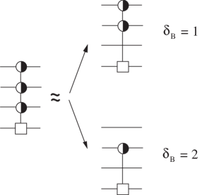
Figure 1: Approximating a $U(2)$-multiplexor by another $U(2)$-multiplexor with $\delta_{B}$ fewer controls.

2 Notation

In this section, we will define some notation that is used throughout this paper. For additional information about our notation, we recommend that the reader consult Ref.[10]. Ref.[10] is a review article, written by the author of this paper, which uses the same notation as this paper.

Let $Bool=\{0,1\}$. As usual, let ${\mathbb{Z}},{\mathbb{R}},{\mathbb{C}}$ represent the set of integers (negative and non-negative), real numbers, and complex numbers, respectively. For integers $a$, $b$ such that $a\leq b$, let ${\mathbb{Z}}_{a,b}=\{a,a+1,\ldots b-1,b\}$. For $\Gamma$ equal to ${\mathbb{Z}}$ or ${\mathbb{R}}$, let $\Gamma^{>0}$ and $\Gamma^{\geq 0}$ represent the set of positive and non-negative $\Gamma$ numbers, respectively. For any positive integer $n$ and any set $S$, let $S^{n}$ denote the Cartesian product of $n$ copies of $S$; i.e., the set of all $n$-tuples of elements of $S$.

For any (not necessarily distinct) objects $a_{1},a_{2},a_{3},\ldots$, let $\{a_{1},a_{2},a_{3},\ldots\}_{ord}$ denote an ordered set. For some object $b$, let $b\{a_{1},a_{2},a_{3},\ldots\}_{ord}=\{ba_{1},ba_{2},ba_{3},\ldots\}_{ord}$. Let $\emptyset$ be the empty set. For an ordered set $S$, let $S^{R}$ be $S$ in reverse order.

We will use $\theta(S)$ to represent the “truth function”; $\theta(S)$ equals 1 if statement $S$ is true and 0 if $S$ is false. For example, the Kronecker delta function is defined by $\delta^{y}_{x}=\delta(x,y)=\theta(x=y)$. For $x\in Bool$,

$$\sum_{k=0}^{1}(-1)^{kx}=2\delta(x,0)\;.$$ (1)

For any positive integer $N$, we will use $\vec{e}_{i}$ where $i=1,2,\ldots,N$ to denote the standard basis vectors in $N$ dimensions; i.e., $[\vec{e}_{i}]_{j}=\delta(i,j)$ for $i,j\in{\mathbb{Z}}_{1,N}$.

$I_{n}$ and $0_{n}$ will represent the $n$-dimensional unit and zero matrices.

For any matrix $A$ and positive integer $n$, let

$$A^{\otimes n}=\underbrace{A\otimes\cdots\otimes A\otimes A}_{n\;\;{\rm copies\;\;of\;\;}A}\;,$$ (2)

$$A^{\oplus n}=\underbrace{A\oplus\cdots\oplus A\oplus A}_{n\;\;{\rm copies\;\;of\;\;}A}\;.$$ (3)

For any matrix $A\in{\mathbb{C}}^{m\times n}$ and $p=1,2,\infty$, $\|A\|_{p}$ will represent the $p$-norm of $A$, and $\|A\|_{F}$ its Frobenius norm. See [11] for a discussion of matrix norms.

Let $\vec{x}\in{\mathbb{C}}^{n\times 1}$. As is customary in the Physics literature, $\|\vec{x}\|_{2}$ will also be denoted by $|\vec{x}|$ and called the magnitude of $\vec{x}$. For any complex matrix $A$, we will use $abs(A)$ to denote the matrix that is obtained from $A$ by replacing each of its entries by its absolute value. In other words, $[abs(A)]_{ij}=abs(A_{ij})=|A_{ij}|$. (Careful: Ref.[11] and many other mathematical books call $|A|$ what we call $abs(A)$).

Any $x\in{\mathbb{R}}$ can be expressed as a doubly infinite power series in powers of a base $E\in{\mathbb{Z}}^{>0}$: $x=\pm\sum_{\alpha=-\infty}^{\infty}x_{\alpha}E^{\alpha}$. This expansion can be represented by: $\pm(\cdots x_{1}x_{0}.x_{-1}x_{-2}\cdots)_{\flat E}$, which is called the base $E$ representation of $x$. The plus or minus in these expressions is chosen to agree with the sign of $x$. It is customary to omit the subscript $\flat E$ when $E=10$. For example $2.25=2+\frac{1}{4}={(1.01)_{\flat 2}}$

Suppose $x={(\cdots x_{1}x_{0}.x_{-1}x_{-2}\cdots)_{\flat 2}}\in{\mathbb{R}}^{\geq 0}$. Note that division by 2 shifts the binary representation of $x$ one space to the right: $\frac{x}{2}={(\cdots x_{1}.x_{0}\cdots)_{\flat 2}}$. Likewise, multiplication by 2 shifts the binary representation of $x$ one space to the left: $2x={(\cdots x_{-1}.x_{-2}\cdots)_{\flat 2}}$. In general, for any $\alpha\in{\mathbb{Z}}$, $\frac{x}{2^{\alpha}}={(\cdots x_{\alpha}.x_{\alpha-1}\cdots)_{\flat 2}}$.

Define the action of an overline placed over an $a\in Bool$ by $\overline{0}=1$ $\overline{1}=0$. Call this bit negation. Define the action of an oplus placed between $a,b\in Bool$ by $a\oplus b=\theta(a\neq b)$. Call this bit addition. One can extend the bit negation and bit addition operations so that they can act on non-negative reals. Suppose $x={(\cdots x_{1}x_{0}.x_{-1}x_{-2}\cdots)_{\flat 2}}$, and $y={(\cdots y_{1}y_{0}.y_{-1}y_{-2}\cdots)_{\flat 2}}$ are non-negative real numbers. Then define the action of an overline over $x$ so that it acts on each bit individually; i.e., so that $[\overline{x}]_{\alpha}=\overline{x_{\alpha}}$. This overline operation is sometimes called bitwise negation. Likewise, define the action of an oplus placed between $x$ and $y$ by $(x\oplus y)_{\alpha}=x_{\alpha}\oplus y_{\alpha}$. This oplus operation is sometimes called bitwise addition (without carry).

For any $x\in{\mathbb{R}}$, the floor function is defined by ${\lfloor x\rfloor}=\max\{j\in{\mathbb{Z}}:j\leq x\}$, and the ceiling function by ${\lceil x\rceil}=\min\{j\in{\mathbb{Z}}:j\geq x\}$. For example, if $x={(\cdots x_{1}x_{0}.x_{-1}x_{-2}\cdots)_{\flat 2}}$, then ${\lfloor x\rfloor}={(\cdots x_{2}x_{1}x_{0})_{\flat 2}}$.

We will often use ${N_{B}}$ to denote a number of bits, and ${N_{S}}=2^{{N_{B}}}$ to denote the corresponding number of states. We will use the sets $Bool^{N_{B}}$ and ${\mathbb{Z}}_{0,{N_{S}}-1}$ interchangeably, since any $x\in{\mathbb{Z}}_{0,{N_{S}}-1}$ can be identified with its binary representation ${(x_{{N_{B}}-1}\cdots x_{1}x_{0})_{\flat 2}}\in Bool^{{N_{B}}}$.

For any $x={(x_{{N_{B}}-1}\cdots x_{1}x_{0})_{\flat 2}}\in{\mathbb{Z}}_{0,{N_{S}}-1}$, define $x^{R}={(x_{0}x_{1}\cdots x_{{N_{B}}-1})_{\flat 2}}$; i.e., $x^{R}$ is the result of reversing the binary representation of $x$.

Suppose $\pi:{\mathbb{Z}}_{0,{N_{S}}-1}\rightarrow{\mathbb{Z}}_{0,{N_{S}}-1}$ is a 1-1 onto map. (We use the letter $\pi$ to remind us it is a permutation; i.e., a 1-1 onto map from a finite set onto itself). One can define a permutation matrix $M$ with entries given by $M_{yx}=\theta(y=\pi(x))$ for all $x,y\in{\mathbb{Z}}_{0,{N_{S}}-1}$. (Recall that all permutation matrices $M$ arise from permuting the columns of the unit matrix, and they satisfy $M^{T}M=1$.) In this paper, we will often represent the map $\pi$ and its corresponding matrix $M$ by the same symbol $\pi$. Whether the function or the matrix is being alluded to will be clear from the context. For example, suppose $A$ is an ${N_{S}}$ dimension matrix, and $\pi$ is a permutation on the set ${\mathbb{Z}}_{0,{N_{S}}-1}$. Then, it is easy to check that for all $i,j\in{\mathbb{Z}}_{0,{N_{S}}-1}$, $(\pi^{T}A)_{ij}=A_{\pi(i),j}$ and $(A\pi)_{ij}=A_{i,\pi(j)}$.

Suppose $\pi_{B}:{\mathbb{Z}}_{0,{N_{B}}-1}\rightarrow{\mathbb{Z}}_{0,{N_{B}}-1}$ is a 1-1 onto map (i.e., a bit permutation). $\pi_{B}$ can be extended to a map $\pi_{B}:{\mathbb{Z}}_{0,{N_{S}}-1}\rightarrow{\mathbb{Z}}_{0,{N_{S}}-1}$ as follows. If $x={(x_{{N_{B}}-1}\cdots x_{1}x_{0})_{\flat 2}}\in{\mathbb{Z}}_{0,{N_{S}}-1}$, then let $[\pi_{B}(x)]_{\alpha}=x_{\pi_{B}(\alpha)}$ for all $\alpha\in{\mathbb{Z}}_{0,{N_{B}}-1}$. The function $\pi_{B}:{\mathbb{Z}}_{0,{N_{S}}-1}\rightarrow{\mathbb{Z}}_{0,{N_{S}}-1}$ is 1-1 onto, so it can be used to define a permutation matrix of the same name. Thus, the symbol $\pi_{B}$ will be used to refer to 3 different objects: a permutation on the set ${\mathbb{Z}}_{0,{N_{B}}-1}$, a permutation on the set ${\mathbb{Z}}_{0,{N_{S}}-1}$, and an ${N_{S}}$ dimensional permutation matrix. All permutations on ${\mathbb{Z}}_{0,{N_{B}}-1}$ generate a permutation on ${\mathbb{Z}}_{0,{N_{S}}-1}$, but not all permutations on ${\mathbb{Z}}_{0,{N_{S}}-1}$ have an underlying permutation on ${\mathbb{Z}}_{0,{N_{B}}-1}$.

An example of a bit permutation that will arise later is $\pi_{R}$; it maps $\pi_{R}(i)=i^{R}$ for all $i\in{\mathbb{Z}}_{0,{N_{S}}-1}$ and $\pi_{R}(\alpha)={N_{B}}-1-\alpha$ for all $\alpha\in{\mathbb{Z}}_{0,{N_{B}}-1}$.

3 Gray Code

In this section, we will review some well known facts about Gray code[12]. (Gray code was named after a person named Gray, not after the color.)

For any positive integer ${N_{B}}$, we define a Grayish code to be a list of the elements of $Bool^{N_{B}}$ such that adjacent ${N_{B}}$-tuples of the list differ in only one component. In other words, a Grayish code is a 1-1 onto map $\pi_{Gish}:{\mathbb{Z}}_{0,{N_{S}}-1}\rightarrow{\mathbb{Z}}_{0,{N_{S}}-1}$ such that, for all $k\in{\mathbb{Z}}_{0,{N_{S}}-2}$, the binary representations of $\pi_{Gish}(k)$ and $\pi_{Gish}(k+1)$ differ in only one component. For any ${N_{B}}>1$, there are many functions $\pi_{Gish}$ that satisfy this definition.

Next we will define a particular Grayish code that we shall refer to as “the” Gray code and denote by $\pi_{G}$. The Gray code for ${N_{B}}=1,2,3$ is:

$$\begin{array}[]{|c|c|c|}\hline\cr k&{(k)_{\flat 2}}&\pi_{G}(k)\\ \hline\cr 0&0&0\\ 1&1&1\\ \hline\cr\end{array}\;\;\begin{array}[]{|c|c|c|}\hline\cr k&{(k)_{\flat 2}}&\pi_{G}(k)\\ \hline\cr 0&00&00\\ 1&01&01\\ 2&10&11\\ 3&11&10\\ \hline\cr\end{array}\;\;\begin{array}[]{|c|c|c|}\hline\cr k&{(k)_{\flat 2}}&\pi_{G}(k)\\ \hline\cr 0&000&000\\ 1&001&001\\ 2&010&011\\ 3&011&010\\ 4&100&110\\ 5&101&111\\ 6&110&101\\ 7&111&100\\ \hline\cr\end{array}\;.$$ (4)

The Gray code can be defined recursively as follows. Let $\Gamma_{0}=\emptyset$. For ${N_{B}}>0$, let $\Gamma_{N_{B}}$ equal the set $Bool^{N_{B}}$ ordered in the Gray code order. In other words, $\Gamma_{N_{B}}=\{\pi_{G}(0),\pi_{G}(1),\pi_{G}(2),\ldots,\pi_{G}(2^{N_{B}}-1)\}_{ord}$. Then,

$$\Gamma_{{N_{B}}+1}=\{0\Gamma_{N_{B}},1\Gamma^{R}_{N_{B}}\}_{ord}\ \;$$ (5)

for ${N_{B}}\in{\mathbb{Z}}_{0,\infty}$.(See Section 2 for ordered set notation.)

From the recursive definition of the Gray code, it is possible to prove that if $k={(\cdots k_{2}k_{1}k_{0})_{\flat 2}}$ and $g={(\cdots g_{2}g_{1}g_{0})_{\flat 2}}$ are nonnegative integers such that $g=\pi_{G}(k)$, then

$$g_{\alpha}=k_{\alpha}\oplus k_{\alpha+1}\;,$$ (6a)

for all $$\alpha\in{\mathbb{Z}}_{0,\infty} \alpha>{N_{B}}-1 k_{\alpha}=g_{\alpha}=0 {N_{B}} {N_{B}} g {N_{B}} k$$. (For all , ). Eq.(6a) specifies linear equations for the components of expressed in terms of the components of . These equations can be easily inverted using Gauss Elimination to get:

$$k_{\alpha}=g_{\alpha}\oplus g_{\alpha+1}\oplus g_{\alpha+2}\oplus g_{\alpha+3}\oplus\cdots\;.$$ (6b)

Eqs.(6) can also be written in terms of the floor function:

$$g=k\oplus{\lfloor\frac{k}{2}\rfloor}\;,$$ (7a)

$$k=g\oplus{\lfloor\frac{g}{2}\rfloor}\oplus{\lfloor\frac{g}{2^{2}}\rfloor}\oplus{\lfloor\frac{g}{2^{3}}\rfloor}\oplus\cdots\;.$$ (7b)

As in Section 2, suppose $\pi_{B}$ represents a permutation on ${\mathbb{Z}}_{0,{N_{B}}-1}$ which generates a permutation on ${\mathbb{Z}}_{0,{N_{S}}-1}$ of the same name. Clearly, $\pi_{B}\circ\pi_{G}$ is a Grayish code. Indeed, $\pi_{B}\circ\pi_{G}$ is a 1-1 onto map, and permuting bits the same way for all elements of a list preserves the property that adjacent ${N_{B}}$-tuples differ in only one component. (Note, however, that it is easy to find $\pi_{B}$’s such that $\pi_{G}\circ\pi_{B}$ is not a Grayish code. Hence, to preserve Grayishness, one must apply the bit permutation after $\pi_{G}$, not before).

4 Hadamard, Paley and Walsh Matrices

In this section, we will review some well known facts about the so called Hadamard, Paley and Walsh matrices (a.k.a. transforms) [12].

For any positive integer ${N_{B}}$, we define the ${N_{B}}$-bit Hadamard matrix by

$$(H_{N_{B}})_{k,r}=\frac{1}{\sqrt{{N_{S}}}}(-1)^{\sum_{\alpha=0}^{{N_{B}}-1}k_{\alpha}r_{\alpha}},\;$$ (8)

the ${N_{B}}$-bit Paley matrix by

$$(P_{N_{B}})_{k,r}=\frac{1}{\sqrt{{N_{S}}}}(-1)^{\sum_{\alpha=0}^{{N_{B}}-1}\sum_{\beta=0}^{{N_{B}}-1}k_{\alpha}r_{\beta}\delta_{\alpha+\beta}^{{N_{B}}-1}},\;$$ (9)

and the ${N_{B}}$-bit Walsh matrix by

$$(W_{N_{B}})_{k,r}=\frac{1}{\sqrt{{N_{S}}}}(-1)^{\sum_{\alpha=0}^{{N_{B}}-1}\sum_{\beta=0}^{{N_{B}}-1}k_{\alpha}r_{\beta}[\delta_{\alpha+\beta}^{{N_{B}}}+\delta_{\alpha+\beta}^{{N_{B}}-1}]}\;,$$ (10)

where $k,r\in{\mathbb{Z}}_{0,2^{N_{B}}-1}$, $k={(\cdots k_{2}k_{1}k_{0})_{\flat 2}}$ and $r={(\cdots r_{2}r_{1}r_{0})_{\flat 2}}$. We will often omit the subscript ${N_{B}}$ from $H_{N_{B}},P_{N_{B}},W_{N_{B}}$ in contexts where doing this does not lead to confusion.

Note that $H,P,W$ are real symmetric matrices.

For $j\in{\mathbb{Z}}_{0,{N_{S}}-1}$, define the “reversal” function $\pi_{R({N_{B}})}(j)=j^{R}$, and the “negation” function $\pi_{N({N_{B}})}(j)=\overline{j}$. The function $\pi_{G({N_{B}})}$ for ${N_{B}}$-bit Gray code has been defined previously. The functions $\pi_{R({N_{B}})}$, $\pi_{N({N_{B}})}$ and $\pi_{G({N_{B}})}$ are 1-1 onto so they can be used to define permutation matrices of the same name (See Section 2.) We will often write $\pi_{R}$, $\pi_{N}$ and $\pi_{G}$ instead of $\pi_{R({N_{B}})}$, $\pi_{N({N_{B}})}$ and $\pi_{G({N_{B}})}$ in contexts where this does not lead to confusion.

Note that $\pi_{R}$ and $\pi_{N}$ are symmetric matrices but $\pi_{G}$ isn’t.

Next we will show that the ${N_{B}}$-bit Hadamard, Paley and Walsh matrices all have the same columns, except in different orders. More specifically, $H,P,W$ are related to each other by the following equations:

$$H\pi_{R}=P\;,\;\;P\pi_{G}=W\;.$$ (11)

A more pictorial way of expressing Eqs.(11) is:

$$H\stackrel{{\scriptstyle(\cdot)\pi_{R}}}{{\longrightarrow}}P\stackrel{{\scriptstyle(\cdot)\pi_{G}}}{{\longrightarrow}}W\;.$$ (12)

Taking the transpose of both sides of Eqs.(11) leads to

$$\pi_{R}H=P\;,\;\;\pi_{G}^{T}P=W\;.$$ (13)

In the last equation, we have used the fact that matrices $H,P,W$, $\pi_{R},\pi_{N}$ are symmetric but $\pi_{G}$ isn’t.

Comparing Eqs.(11) and (13), we see that

$$H\pi_{R}=\pi_{R}H\;,$$ (14)

and

$$P\pi_{G}=\pi_{G}^{T}P\;.$$ (15)

In fact, Eq.(14) can be generalized as follows. Suppose $\pi_{B}$ is a bit permutation on ${\mathbb{Z}}_{0,{N_{B}}-1}$. Then

$$(\pi_{B}^{T}H\pi_{B})_{kr} = H_{\pi_{B}(k),\pi_{B}(r)}$$ (16a)

$$= \frac{1}{\sqrt{{N_{S}}}}(-1)^{\sum_{\alpha=0}^{{N_{B}}-1}[\pi_{B}(k)]_{\alpha}[\pi_{B}(r)]_{\alpha}}$$ (16b)

$$= \frac{1}{\sqrt{{N_{S}}}}(-1)^{\sum_{\alpha=0}^{{N_{B}}-1}k_{\pi(\alpha)}r_{\pi(\alpha)}}$$ (16c)

$$= H_{kr}\;,$$ (16d)

so

$$H\pi_{B}=\pi_{B}H\;.$$ (17)

Eq.(17) becomes Eq.(14) when $\pi_{B}=\pi_{R}$.

To prove Eqs.(11), note that

$$(H\pi_{R})_{ik} = \sum_{j=0}^{{N_{S}}-1}H_{ij}(\pi_{R})_{jk}$$ (18a)

$$= \frac{1}{\sqrt{{N_{S}}}}\sum_{j}(-1)^{\sum_{\alpha}i_{\alpha}j_{\alpha}}\theta(j=k^{R})$$ (18b)

$$= P_{ik}\;.$$ (18c)

Similarly,

$$(P\pi_{G})_{ik} = \sum_{j=0}^{{N_{S}}-1}P_{ij}(\pi_{G})_{jk}$$ (19a)

$$= \frac{1}{\sqrt{{N_{S}}}}\sum_{j}(-1)^{\sum_{\alpha,\beta}i_{\alpha}j_{\beta}\delta_{\alpha+\beta}^{{N_{B}}-1}}\theta(j=\pi_{G}(k))$$ (19b)

$$= \frac{1}{\sqrt{{N_{S}}}}(-1)^{\sum_{\alpha,\beta}i_{\alpha}(k_{\beta}\oplus k_{\beta+1})\delta_{\alpha+\beta}^{{N_{B}}-1}}$$ (19c)

$$= \frac{1}{\sqrt{{N_{S}}}}(-1)^{\sum_{\alpha}i_{\alpha}(k_{{N_{B}}-1-\alpha}+k_{{N_{B}}-\alpha})}$$ (19d)

$$= W_{ik}\;.$$ (19e)

The square of $H,P$ and $W$ is one. Indeed, using Eq.(1) we get

$$(H^{2})_{ik} = \sum_{j=0}^{{N_{S}}-1}H_{ij}H_{jk}$$ (20a)

$$= \frac{1}{2^{{N_{B}}}}\sum_{j_{{N_{B}}-1}=0}^{1}\ldots\sum_{j_{1}=0}^{1}\sum_{j_{0}=0}^{1}(-1)^{\sum_{\alpha=0}^{{N_{B}}-1}(i_{\alpha}+k_{\alpha})j_{\alpha}}$$ (20b)

$$= \prod_{\alpha}\delta_{i_{\alpha}}^{k_{\alpha}}=\delta_{i}^{k}\;,$$ (20c)

$$P^{2}=(\pi_{R}H)(H\pi_{R})=1\;,$$ (21)

and

$$W^{2}=(\pi_{G}^{T}P)(P\pi_{G})=1\;.$$ (22)

Since their square equals one, and they are real symmetric matrices, $H,P$ and $W$ are also orthogonal matrices.

From the definitions given above for $\pi_{R},\pi_{N},\pi_{G}$, one can prove by induction on ${N_{B}}$ that these matrices obey the following recursive equations:

$$\pi_{R(0)}=1\;,\;\;\pi_{R({N_{B}}+1)}=\left[\begin{array}[]{c}\pi_{R({N_{B}})}\otimes(1,0)\\ \pi_{R({N_{B}})}\otimes(0,1)\end{array}\right]\;,$$ (23a)

$$\pi_{N(0)}=1\;,\;\;\pi_{N({N_{B}}+1)}=\pi_{N({N_{B}})}\otimes\left[\begin{array}[]{cc}0&1\\ 1&0\end{array}\right]\;,$$ (23b)

and

$$\pi_{G(0)}=1\;,\;\;\pi_{G({N_{B}}+1)}=\left[\begin{array}[]{cc}\pi_{G({N_{B}})}&0\\ 0&\pi_{G({N_{B}})}\pi_{N({N_{B}})}\end{array}\right]\;.$$ (23c)

Similarly, from the definitions given above for $H,P,W$, one can prove by induction on ${N_{B}}$ that these matrices obey the following recursive equations:

$$H_{0}=1\;,\;\;H_{{N_{B}}+1}=H_{{N_{B}}}\otimes\left[\begin{array}[]{cc}1&1\\ 1&-1\end{array}\right]\frac{1}{\sqrt{2}}\;,$$ (24a)

$$P_{0}=1\;,\;\;P_{{N_{B}}+1}=\left[\begin{array}[]{cc}P_{{N_{B}}}\otimes(1,1)\\ P_{{N_{B}}}\otimes(1,-1)\end{array}\right]\frac{1}{\sqrt{2}}\;,$$ (24b)

and

$$W_{0}=1\;,\;\;W_{{N_{B}}+1}=\left[\begin{array}[]{cc}W_{{N_{B}}}\otimes(1,1)\\ (\pi_{N({N_{B}})}W_{{N_{B}}})\otimes(1,-1)\end{array}\right]\frac{1}{\sqrt{2}}\;.$$ (24c)

By virtue of Eqs.(11),

$$W=H\pi_{R}\pi_{G}\;,$$ (25)

Eq.(25) means that the permutation $\pi_{R}\pi_{G}$ will permute the columns of $H$ to give $W$. Expressing Eq.(25) in component form, we find

$$W_{ij} = \sum_{r,k}H_{ir}(\pi_{R})_{rk}(\pi_{G})_{kj}$$ (26a)

$$= \sum_{r,k}H_{ir}\theta(r=\pi_{R}(k))\theta(k=\pi_{G}(j))$$ (26b)

$$= H_{i,\pi_{R}\circ\pi_{G}(j)}\;.$$ (26c)

Thus, if we denote the columns of $H_{N_{B}}$ and $W_{N_{B}}$ by $\vec{h}_{j}$ and $\vec{w}_{j}$, respectively, then

$$\vec{w}_{j}=\vec{h}_{\pi_{R}\circ\pi_{G}(j)}\;,$$ (27)

for $j\in{\mathbb{Z}}_{0,{N_{S}}-1}$.

5 Constancy

In this section, we will define a property of vectors called constancy. The columns of $H_{N_{B}}$ can be conveniently classified according to their constancy.

Consider the 3-bit Hadamard matrix:

$$H_{3}=H_{1}^{\otimes 3}=\frac{1}{\sqrt{2^{3}}}\begin{array}[]{|rrrrrrrr|}{\scriptstyle\vec{h}_{000}}&{\scriptstyle\vec{h}_{001}}&{\scriptstyle\vec{h}_{010}}&{\scriptstyle\vec{h}_{011}}&{\scriptstyle\vec{h}_{100}}&{\scriptstyle\vec{h}_{101}}&{\scriptstyle\vec{h}_{110}}&{\scriptstyle\vec{h}_{111}}\\ \hline\cr+1&+1&+1&+1&+1&+1&+1&+1\\ +1&-1&+1&-1&+1&-1&+1&-1\\ +1&+1&-1&-1&+1&+1&-1&-1\\ +1&-1&-1&+1&+1&-1&-1&+1\\ +1&+1&+1&+1&-1&-1&-1&-1\\ +1&-1&+1&-1&-1&+1&-1&+1\\ +1&+1&-1&-1&-1&-1&+1&+1\\ +1&-1&-1&+1&-1&+1&+1&-1\\ \hline\cr\end{array}\;,$$ (28)

where we have labelled the columns of $H_{3}$ by $\vec{h}_{j}$, where the index $j$ is given in its binary representation. According to Eq.(27), to get $W_{3}$ from Eq.(28), one can simply reorder the columns of $H_{3}$ in bit-reversed Gray code. The columns of $H_{3}$ (and of $W_{3}$) can be classified according to their constancy. We define the constancy ${\cal C}(\vec{h})$ of a vector $\vec{h}$ to be the smallest number of identical adjacent entries of $\vec{h}$. For example, ${\cal C}([1,-1,1,1]^{T})=1$ and ${\cal C}([1,1,-1,-1]^{T})=2$. The next table gives the constancy of the columns of $H_{3}$, with the columns listed in the order in which they appear in $W_{3}$.

$$\begin{array}[]{|l|l|l|l|}\hline\cr k&\pi_{G}(k)&\pi_{R}\circ\pi_{G}(k)&{\cal C}[\vec{h}_{\pi_{R}\circ\pi_{G}(k)}]\\ \hline\cr\hline\cr 000&000&000&8\\ \hline\cr 001&001&100&4\\ \hline\cr 010&011&110&2\\ \hline\cr 011&010&010&2\\ \hline\cr 100&110&011&1\\ \hline\cr 101&111&111&1\\ \hline\cr 110&101&101&1\\ \hline\cr 111&100&001&1\\ \hline\cr\end{array}\;.$$ (29)

It is clear from Eq.(29) that the columns of $W_{3}$ are listed in order of non-increasing constancy, and that the constancies of the columns of $W_{3}$ are all powers of 2. The literature on Walsh matrices often refers to the index that labels the columns of $W$ as the sequency of that column. Thus, as sequency increases, constancy decreases or stays the same. Sequency and Constancy are analogous to Frequency and Period, respectively, in Fourier Analysis.

Note that given any matrix $A$, more than one of the columns of $A$ may have the same constancy. We will refer to: the number of columns of $A$ with the same constancy $K$, as: the multiplicity of the constancy $K$ in the matrix $A$, and denote it by ${\cal M}_{A}({\cal C}=K)$. In this paper, we are only concerned with the case where $A$ equals the ${N_{B}}$-bit Hadamard matrix so we will henceforth omit the subscript $A$ from ${\cal M}_{A}({\cal C}=K)$. Sometimes we will also abbreviate ${\cal M}({\cal C}=K)$ by ${\cal M}(K)$, if doing this does not lead to confusion. The next table gives the multiplicity of the constancy $K$ in the ${N_{B}}$-bit Hadamard matrix:

$$\begin{array}[]{l|lllll}{\cal M}({\cal C}=K)&K=1&K=2&K=4&K=8&\cdots\\ \hline\cr{N_{B}}=1&1&1&0&0&\cdots\\ {N_{B}}=2&2&1&1&0&\cdots\\ {N_{B}}=3&4&2&1&1&\cdots\\ \vdots&\vdots&\vdots&\vdots&\vdots&\vdots\\ \end{array}\;.$$ (30)

It is also convenient to define

$${\cal M}({\cal C}\geq{N_{S}}^{\prime})=\sum_{K\geq{N_{S}}^{\prime}}{\cal M}(K)\;.$$ (31)

We shall call this the cumulative multiplicity of the constancy. The next table can be easily obtained from Eq.(30) and Eq.(31). It gives ${\cal M}({\cal C}\geq{N_{S}}^{\prime})$ for the ${N_{B}}$-bit Hadamard matrix.

$$\begin{array}[]{l|lllll}{\cal M}({\cal C}\geq{N_{S}}^{\prime})&{N_{S}}^{\prime}=2^{0}&{N_{S}}^{\prime}=2^{1}&{N_{S}}^{\prime}=2^{2}&{N_{S}}^{\prime}=2^{3}&\cdots\\ \hline\cr{N_{B}}=1&2&1&0&0&\cdots\\ {N_{B}}=2&4&2&1&0&\cdots\\ {N_{B}}=3&8&4&2&1&\cdots\\ \vdots&\vdots&\vdots&\vdots&\vdots&\vdots\\ \end{array}\;.$$ (32)

It is clear from Eq.(32) that ${\cal M}({\cal C}\geq{N_{S}}^{\prime})=2^{{N_{B}}-{N_{B}}^{\prime}}\theta({N_{B}}\geq{N_{B}}^{\prime})$, where ${N_{S}}^{\prime}=2^{{N_{B}}^{\prime}}$.

6 Symmetries of Multiplexors

In this section, we discuss some symmetries of exact decompositions of $U(2)$-multiplexors.

For simplicity, we will first consider the $R_{y}(2)$-multiplexors used in Ref.[5]. Ref.[6] uses $U(2)$-multiplexors that are more general than the $R_{y}(2)$-multiplexors used in Ref.[5]. At the end of the paper, we will discuss how to generalize our results for $R_{y}(2)$-multiplexors so that they apply to the more general multiplexors used in Ref.[6].

Below, we will present some quantum circuit diagrams. Besides the circuit notational conventions defined in Refs.[6] and [10], the circuits below will use the following additional notation. A square gate with an angle $\theta$ below the square will represent $\exp(i\theta{\sigma_{y}})$ applied at that “wire”. Typically, we will consider a SEO consisting of alternating one-qubit rotations and CNOTs. The SEO will always have a one-qubit rotation at one end and a CNOT at the other. The angle for the one-qubit rotation that either begins or ends the SEO will be denoted by $\theta_{00\ldots 0}$. Given two adjacent angles $\theta_{b}$ and $\theta_{b^{\prime}}$ in the SEO, ${(b)_{\flat 2}}$ and ${(b^{\prime})_{\flat 2}}$ will differ only in one component, component $\alpha$, where $\alpha$ is the position of the control bit of the CNOT that lies between the $\theta_{b}$ and $\theta_{b^{\prime}}$ gates.

If we take the Hermitian conjugate of the multiplexor $\exp(i\sum_{b\in Bool^{{N_{B}}-1}}\phi_{b}{\sigma_{y}}\otimes P_{b})$, and then we replace the angles $\phi_{b}$ by their negatives (and also the angles $\theta_{b}$, Hadamard transforms of the $\phi_{b}$, by their negatives), we get the same multiplexor back. Henceforth, we will refer to this symmetry transformation as time reversal. Thus, an $R_{y}(2)$-multiplexor is invariant under time reversal.

Suppose $\pi_{B}$ is a bit permutation on ${N_{B}}-1$ bits. If we replace $\phi_{b}$ by $\phi_{\pi_{B}(b)}$ (and also $\theta_{b}$ by $\theta_{\pi_{B}(b)}$) and $P_{b}$ by $P_{\pi_{B}(b)}$ in the multiplexor $\exp(i\sum_{b\in Bool^{{N_{B}}-1}}\phi_{b}{\sigma_{y}}\otimes P_{b})$, we get the same multiplexor back. Henceforth, we will refer to this symmetry transformation as bit permutation. Thus, an $R_{y}(2)$-multiplexor is also invariant under bit permutation.

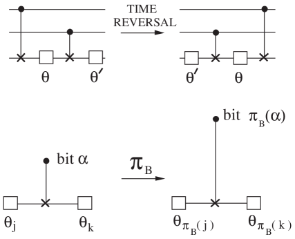
Figure 2: Examples of the action of time reversal and bit permutation on a string of one-qubit rotations and CNOTs.

Fig.2 shows how time reversal and bit permutation act on a sequence of one-qubit rotations and CNOTs. More examples of the application of these transformations will be given below.

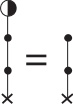
Figure 3: A half-moon node represents a projector $P_{b}$ where $b\in Bool$. The half-moon node may be omitted when it appears in a multiplexor whose $U(2^{N_{T}})$-subset does not depend on the index $b$. This figure is an example of this principle.

Recall from Ref.[6] our definition of a general multiplexor with $N_{K}$ control qubits $\vec{\kappa}$ and $N_{T}$ target qubits $\vec{\tau}$: $\sum_{{b}\in Bool^{N_{K}}}U_{b}(\vec{\tau})P_{b}(\vec{\kappa})$. In a multiplexor whose matrices $U_{b}$ are independent of the $\alpha$ component $b_{\alpha}$ of $b$, we can sum $P_{b_{\alpha}}$ over $b_{\alpha}\in Bool$ to get 1. Such a multiplexor acts as the identity on qubit $\alpha$. When representing such a multiplexor in a circuit diagram, we can omit its half-moon node on qubit line $\alpha$. Fig.3 shows a very special case of this principle, a special case that will be used in the circuit diagrams below.

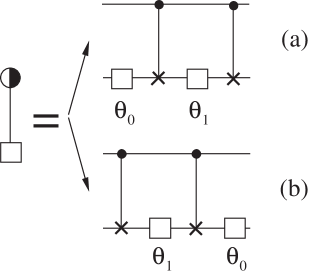
Figure 4: Two possible decompositions of an $R_{y}(2)$-multiplexor with 1 control.

Fig.4 shows two possible ways of decomposing an $R_{y}(2)$-multiplexor with one control. The decomposition (a) in Fig.4 is equivalent to:

$$\exp\left(i\sum_{b\in Bool}\phi_{b}{\sigma_{y}}\otimes P_{b}\right)=e^{i\theta_{0}{\sigma_{y}}(1)}{\sigma_{x}}(1)^{n(0)}e^{i\theta_{1}{\sigma_{y}}(1)}{\sigma_{x}}(1)^{n(0)}\;.$$ (33)

Let LHS and RHS stand for the left and right hand sides of Eq.(33). Recall that $n=diag(0,1)=P_{1}$ and ${\overline{n}}=1-n=diag(1,0)=P_{0}$. Eq.(33) can be proven as follows:

$$RHS = e^{i\theta_{0}{\sigma_{y}}(1)}e^{i\theta_{1}{\sigma_{y}}(1){\sigma_{z}}(0)}$$ (34a)

$$= e^{i{\sigma_{y}}(1)\{\theta_{0}+\theta_{1}[P_{0}(0)-P_{1}(0)]\}}$$ (34b)

$$= LHS\;.$$ (34c)

To arrive at Eq.(34c), we expressed $\theta_{0},\theta_{1}$ in terms of $\phi_{0},\phi_{1}$ using

$$\left[\begin{array}[]{c}\theta_{0}\\ \theta_{1}\end{array}\right]=\frac{1}{2}\left[\begin{array}[]{rr}1&1\\ 1&-1\end{array}\right]\left[\begin{array}[]{c}\phi_{0}\\ \phi_{1}\end{array}\right]\;.$$ (35)

If we take the Hermitian conjugate of both sides of Eq.(33), and then we replace the angles $\phi_{b}$ and $\theta_{b}$ by their negatives, we get

$$\exp\left(i\sum_{b\in Bool}\phi_{b}{\sigma_{y}}\otimes P_{b}\right)={\sigma_{x}}(1)^{n(0)}e^{i\theta_{1}{\sigma_{y}}(1)}{\sigma_{x}}(1)^{n(0)}e^{i\theta_{0}{\sigma_{y}}(1)}\;.$$ (36)

Eq.(36) is equivalent to decomposition (b) in Fig.4. Thus, decompositions (a) and (b) in Fig.4 transform into each other under time reversal.

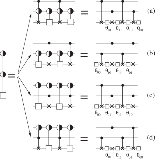
Figure 5: Four possible decompositions of an $R_{y}(2)$-multiplexor with 2 controls.

Fig.5 shows four possible ways of decomposing an $R_{y}(2)$-multiplexor with two controls. Fig.5 was obtained by applying the results of Figs.3 and 4.

In Fig.5, note that decompositions (a) and (b) transform into each other under time reversal. Decompositions (c) and (d) do too. Furthermore, decompositions (b) and (c) transform into each other under bit permutation.

The decompositions exhibited in Fig.5 can also be expressed analytically. For example, decomposition (b) is equivalent to:

$$\exp\left(i\sum_{b\in Bool^{2}}\phi_{b}{\sigma_{y}}\otimes P_{b}\right)=$$ (37)

$$e^{i\theta_{00}{\sigma_{y}}(2)}{\sigma_{x}}(2)^{n(1)}e^{i\theta_{10}{\sigma_{y}}(2)}{\sigma_{x}}(2)^{n(0)}e^{i\theta_{11}{\sigma_{y}}(2)}{\sigma_{x}}(2)^{n(1)}e^{i\theta_{01}{\sigma_{y}}(2)}{\sigma_{x}}(2)^{n(0)}\;.$$

Eq.(37) can be proven using the same techniques that were employed in Eqs.(34) to prove Eq.(33). The proof requires that we assume:

$$\left[\begin{array}[]{c}\theta_{00}\\ \theta_{01}\\ \theta_{10}\\ \theta_{11}\end{array}\right]=\frac{1}{4}\left[\begin{array}[]{rrrr}1&1&1&1\\ 1&-1&1&-1\\ 1&1&-1&-1\\ 1&-1&-1&1\end{array}\right]\left[\begin{array}[]{c}\phi_{00}\\ \phi_{01}\\ \phi_{10}\\ \phi_{11}\end{array}\right]\;.$$ (38)

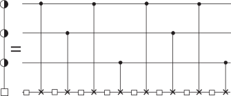
Figure 6: One of several possible decompositions of an $R_{y}(2)$-multiplexor with 3 controls.

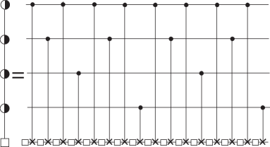
Figure 7: One of several possible decompositions of an $R_{y}(2)$-multiplexor with 4 controls.

Fig. 6 (ditto, 7) shows one of several possible decompositions of an $R_{y}(2)$-multiplexor with 3 (ditto, 4) controls. In general, decompositions for multiplexors with $N_{K}$ controls can be obtained starting from decompositions for multiplexors with $N_{K}-1$ controls.

7 Approximation of Multiplexors

In this section, we finally define our approximation of multiplexors. We give the number of CNOTs required to express the approximant, and an upper bound to the error incurred by using it.

So far we have used ${N_{B}}$ to denote a number of bits, and ${N_{S}}=2^{N_{B}}$ to denote the corresponding number of states. Below, we will use two other numbers of bits, ${\eta_{B}}$ and ${\eta_{B}}^{\prime}$, where ${\eta_{B}}={N_{B}}-1$ and ${\eta_{B}}^{\prime}\leq{\eta_{B}}$. Their corresponding numbers of states will be denoted by ${\eta_{S}}=2^{\eta_{B}}$ and ${\eta_{S}}^{\prime}=2^{{\eta_{B}}^{\prime}}$.

Define an ${\eta_{S}}$ dimensional matrix $V$ by

$$V=H\pi_{B}\pi_{G}\;,$$ (39)

where $\pi_{B}$ is an arbitrary bit permutation on ${\eta_{B}}$ bits. Eq.(39) is a generalization of Eq.(25). Both equations define a new matrix (either $V$ or the Walsh matrix $W$) by permuting the columns of the Hadamard matrix $H$. $V$ becomes $W$ if we specialize the bit permutation $\pi_{B}$ to $\pi_{R}$. If we denote the columns of $V$ by $\vec{v}_{j}$ for $j\in{\mathbb{Z}}_{0,{\eta_{S}}-1}$, then

$$\vec{v}_{j}=\vec{h}_{\pi_{B}\circ\pi_{G}(j)}\;,$$ (40)

which is the counterpart of Eq.(27).

In Ref.[5], the decomposition of an $R_{y}(2)$ multiplexor starts by taking the following Hadamard transform:

$$\vec{\theta}=\frac{1}{\sqrt{{\eta_{S}}}}H_{{\eta_{B}}}\vec{\phi}\;,$$ (41)

where ${\eta_{B}}=N_{B}-1$ and ${\eta_{S}}=2^{\eta_{B}}$. The vectors $\{\vec{v}_{i}\}_{\forall i}$ constitute an orthonormal basis for the space ${\mathbb{R}}^{{\eta_{S}}}$ in which $\vec{\phi}$ lives, so $\vec{\phi}$ can always be expanded in terms of them:

$$\vec{\phi}=\sum_{i=0}^{{\eta_{S}}-1}\vec{v}_{i}({\vec{v}_{i}}^{\dagger}\vec{\phi})\;.$$ (42)

Now suppose that we truncate this expansion, keeping only the first ${\eta_{S}}^{\prime}$ terms, where ${\eta_{S}}^{\prime}=2^{{\eta_{B}}^{\prime}}$ and ${\eta_{B}}^{\prime}\in{\mathbb{Z}}_{0,{N_{B}}-1}$. Let us call $\vec{\phi^{\prime}}$ the resulting approximation to $\vec{\phi}$:

$$\vec{\phi^{\prime}}=\sum_{i=0}^{{\eta_{S}}^{\prime}-1}\vec{v}_{i}({\vec{v}_{i}}^{\dagger}\vec{\phi})\;.$$ (43)

Define $\vec{\theta^{\prime}}$, an approximation to $\vec{\theta}$, as follows:

$$\vec{\theta^{\prime}}=\frac{1}{\sqrt{{\eta_{S}}}}H_{{\eta_{B}}}\vec{\phi^{\prime}}\;.$$ (44)

If we let $\{\vec{e}_{i}\}_{\forall i}$ denote the standard basis vectors, then

$$H_{{\eta_{B}}}\vec{v}_{i}=\left[\begin{array}[]{c}\vec{h}_{0}^{\dagger}\\ \vec{h}_{1}^{\dagger}\\ \vdots\end{array}\right]\vec{h}_{\pi_{B}\circ\pi_{G}(i)}=\vec{e}_{\pi_{B}\circ\pi_{G}(i)}\;.$$ (45)

Therefore,

$$\vec{\theta^{\prime}}=\frac{1}{\sqrt{{\eta_{S}}}}\sum_{i=0}^{{\eta_{S}}^{\prime}-1}\vec{e}_{\pi_{B}\circ\pi_{G}(i)}({\vec{v}_{i}}^{\dagger}\vec{\phi})\;.$$ (46)

By virtue of Eq.(46), if we list the components $\{\theta^{\prime}_{b}\}_{\forall b}$ of $\vec{\theta^{\prime}}$ in the Grayish code order specified by the map $\pi_{B}\circ\pi_{G}$, then the items in the list at positions from ${\eta_{S}}^{\prime}$ to the end of the list are zero. Consider, for example, Fig.5, which gives the exact decompositions for a multiplexor with 2 controls. Suppose that in one of those decompositions, the angles $\theta_{b}$’s in the second half (i.e., the half that does not contain $\theta_{00}$) of the decomposition are all zero. Then the one-qubit rotations in the second half of the decomposition become the identity. Then the three CNOTs in the second half of the decomposition cancel each other in pairs except for one CNOT that survives. The net effect is that the decomposition for a multiplexor with 2 controls degenerates into a decomposition for a multiplexor with only 1 control. The number of control bits is reduced by one in this example. In general, we can approximate a $U(2)$-multiplexor by another $U(2)$-multiplexor (the “approximant”) that has fewer controls, and, therefore, is expressible with fewer CNOTs. We will call the reduction in the number of control bits the bit deficit $\delta_{B}$. Hence, $\delta_{B}={\eta_{B}}-{\eta_{B}}^{\prime}$.

If $N_{CNOT}$ denotes the number of CNOTs in an approximant with bit deficit $\delta_{B}$, then it is clear from Figs.4, 5, 6 and 7 that:

$$\begin{array}[]{|l|l|l|l|l|l|l|}\hline\cr\delta_{B}=&0&1&2&\cdots&{N_{B}}-2&{N_{B}}-1\\ \hline\cr N_{CNOT}=&2^{{N_{B}}-1}&2^{{N_{B}}-2}&2^{{N_{B}}-3}&\cdots&2&0\\ \hline\cr\end{array}\;.$$ (47)

Hence, for $\delta_{B}\in\mathbb{Z}_{0,{N_{B}}-2}$, $N_{CNOT}=2^{{N_{B}}-1-\delta_{B}}$, but for $\delta_{B}={N_{B}}-1$, $N_{CNOT}=0$.

The bit permutation $\pi_{B}$ on which the approximation of a multiplexor depends can be chosen according to various criteria. If we choose $\pi_{B}=\pi_{R}$, then our approximation will keep only the higher constancy components of $\vec{\phi}$. Such a smoothing, high constancies approximation might be useful for some tasks. Similarly, if we choose $\pi_{B}=1$, then our approximation will keep only the lower constancy components of $\vec{\phi}$, giving a low constancies approximation. Alternatively, we could use for $\pi_{B}$ a bit permutation, out of all possible bit permutations on ${\eta_{B}}$ bits, that minimizes the distance between the original multiplexor and its approximant. Such a dominant constancies approximation is useful if our goal is to minimize the error incurred by the approximation.

The error incurred by approximating a multiplexor can be bounded above as follows. Let $\{e^{i\phi_{b}{\sigma_{y}}}\}_{\forall b\in Bool^{{\eta_{B}}}}$ denote the $R_{y}(2)$-subset of an $R_{y}(2)$-multiplexor $\Upsilon$ and $\{e^{i\phi_{b}^{\prime}{\sigma_{y}}}\}_{\forall b\in Bool^{{\eta_{B}}}}$ that of its approximant $\Upsilon^{\prime}$. Call $\|\Upsilon^{\prime}-\Upsilon\|_{2}$ the error of approximating $\Upsilon$ by $\Upsilon^{\prime}$. Note that

$$\|\Upsilon^{\prime}-\Upsilon\|_{2} = \|\oplus_{b\in Bool^{{\eta_{B}}}}(e^{i\phi^{\prime}_{b}{\sigma_{y}}}-e^{i\phi_{b}{\sigma_{y}}})\|_{2}$$ (48a)

$$= \max_{b}\|e^{i\phi^{\prime}_{b}{\sigma_{y}}}-e^{i\phi_{b}{\sigma_{y}}}\|_{2}$$ (48b)

$$\leq \max_{b}|\phi^{\prime}_{b}-\phi_{b}|=\|\vec{\phi^{\prime}}-\vec{\phi}\|_{\infty}\;.$$ (48c)

To arrive at step Eq.(48c), we used the results of Appendix A. We will sometimes refer to $\|\vec{\phi^{\prime}}-\vec{\phi}\|_{\infty}$ as the linearized error, to distinguish it from the error $\|\Upsilon^{\prime}-\Upsilon\|_{2}$.

A simple picture emerges from all this. The error $\epsilon$ and the number of CNOTs $N_{CNOT}$ are two costs that we would like to minimize. These two costs are fungible to a certain extent. Given a multiplexor $\Upsilon$, and an upper bound $\epsilon_{0}$ on $\epsilon$, we can use Eqs.(47) and (48) to find the approximant $\Upsilon^{\prime}$ with the smallest $N_{CNOT}$. Similarly, given a multiplexor $\Upsilon$, and an upper bound $(N_{CNOT})_{0}$ on $N_{CNOT}$, we can use Eqs.(47) and (48) to find the approximant $\Upsilon^{\prime}$ with the smallest $\epsilon$.

At this point we encourage the reader to read Appendix B. It discusses the output of a computer program that calculates $\vec{\phi^{\prime}}$ from $\vec{\phi}$ via Eq.(43).

Next we will show that Eq.(43) can be simplified considerably by taking into account the explicit values of the column vectors $\vec{v}_{j}$.

To get a quick glimpse of the simplification we seek, consider first the special case ${\eta_{B}}=2$. We have

$$H_{2}=\frac{1}{2}\begin{array}[]{|rrrr|}{\scriptstyle\vec{h}_{00}}&{\scriptstyle\vec{h}_{01}}&{\scriptstyle\vec{h}_{10}}&{\scriptstyle\vec{h}_{11}}\\ \hline\cr+1&+1&+1&+1\\ +1&-1&+1&-1\\ +1&+1&-1&-1\\ +1&-1&-1&+1\\ \hline\cr\end{array}\;,\;\;W_{2}=\frac{1}{2}\begin{array}[]{|rrrr|}{\scriptstyle\vec{h}_{00}}&{\scriptstyle\vec{h}_{10}}&{\scriptstyle\vec{h}_{11}}&{\scriptstyle\vec{h}_{01}}\\ \hline\cr+1&+1&+1&+1\\ +1&+1&-1&-1\\ +1&-1&-1&+1\\ +1&-1&+1&-1\\ \hline\cr\end{array}\;.$$ (49)

Define a matrix $\mu$ by

$$\mu=\left(\begin{array}[]{cc}1&1\\ 1&1\end{array}\right)\;.$$ (50)

For any matrix $A$, let $A(:,i:j)$ be the submatrix of $A$ obtained by keeping only its columns from $i$ to $j$. It is easy to check that

$$W_{2}(:,0:3)W_{2}(:,0:3)^{T}=diag(1,1,1,1)\;,$$ (51)

$$W_{2}(:,0:1)W_{2}(:,0:1)^{T}=\frac{1}{2}\left(\begin{array}[]{cc}\mu&0\\ 0&\mu\end{array}\right)=\frac{1}{2}(\mu\oplus\mu)\;,$$ (52)

and

$$W_{2}(:,0:0)W_{2}(:,0:0)^{T}=\frac{1}{4}\left(\begin{array}[]{cc}\mu&\mu\\ \mu&\mu\end{array}\right)=\frac{1}{4}(\mu\otimes\mu)\;.$$ (53)

In each case, we formed a “decimated matrix” $W(:,0:{\eta_{S}}^{\prime}-1)$ from $W$, where ${\eta_{S}}^{\prime}=2^{{\eta_{B}}^{\prime}}$. Then we showed that the projection operator $W(:,0:{\eta_{S}}^{\prime}-1)W(:,0:{\eta_{S}}^{\prime}-1)^{T}$ onto the column space of the decimated matrix, is a matrix whose entries are all either 0 or $\frac{1}{2^{\delta_{B}}}$, and these entries sum to one along each row (or column). Given a set $S$ of real numbers, and given $S_{1}\subset S$, call the average of the elements of $S_{1}$ a “partial average” of the elements of $S$. For example, if ${\eta_{S}}^{\prime}=2$ and $\pi_{B}=\pi_{R}$, then $V=W$ and $\vec{\phi^{\prime}}=W_{2}(:,0:1)W_{2}(:,0:1)^{T}\vec{\phi}$. From Eq.(52), the entries of $\vec{\phi^{\prime}}$ are partial averages of the entries of $\vec{\phi}$.

Next we show how to simplify Eq.(43) for arbitrary ${\eta_{B}}$, not just for ${\eta_{B}}=2$.

Define an ${\eta_{S}}$ dimensional matrix $\Gamma^{({\eta_{B}},{\eta_{B}}^{\prime})}$ by

$$\Gamma^{({\eta_{B}},{\eta_{B}}^{\prime})}_{qs}=\sum_{r=0}^{{\eta_{S}}^{\prime}-1}(W_{\eta_{B}})_{qr}(W_{\eta_{B}}^{T})_{rs}\;.$$ (54)

Below, we will show that $\Gamma^{({\eta_{B}},{\eta_{B}}^{\prime})}$ reduces to:

$$\Gamma^{({\eta_{B}},{\eta_{B}}^{\prime})}_{qs}=\frac{1}{2^{\delta_{B}}}\theta({\lfloor\frac{q}{2^{\delta_{B}}}\rfloor}={\lfloor\frac{s}{2^{\delta_{B}}}\rfloor})\;.$$ (55)

For example, when ${\eta_{B}}=2,{\eta_{B}}^{\prime}=1$, Eq.(55) becomes

$$\left[\Gamma^{(2,1)}_{qs}\right]=\frac{1}{2}\left[\theta({\lfloor\frac{q}{2}\rfloor}={\lfloor\frac{s}{2}\rfloor})\right]=\frac{1}{2}\begin{array}[]{c|cccc}&{\scriptscriptstyle 00}&{\scriptscriptstyle 01}&{\scriptscriptstyle 10}&{\scriptscriptstyle 11}\\ \hline\cr{\scriptscriptstyle 00}&1&1&0&0\\ {\scriptscriptstyle 01}&1&1&0&0\\ {\scriptscriptstyle 10}&0&0&1&1\\ {\scriptscriptstyle 11}&0&0&1&1\end{array}\;.$$ (56)

Eqs.(54) and (55) are given in component form. The identical statements written in matrix form are, respectively,

$$\Gamma^{({\eta_{B}},{\eta_{B}}^{\prime})} = W_{\eta_{B}}(:,0:{\eta_{S}}^{\prime}-1)W_{\eta_{B}}(:,0:{\eta_{S}}^{\prime}-1)^{T}$$ (57a)

$$= W_{\eta_{B}}\left[\begin{array}[]{cc}I_{{\eta_{S}}^{\prime}}&0\\ 0&0_{{\eta_{S}}-{\eta_{S}}^{\prime}}\end{array}\right]W_{\eta_{B}}^{T}\;,$$ (57d)

and

$$\Gamma^{({\eta_{B}},{\eta_{B}}^{\prime})}=\frac{1}{2^{\delta_{B}}}(\mu^{\otimes\delta_{B}})^{\oplus{\eta_{S}}^{\prime}}\;.$$ (58)

Eq.(55) can be proven from Eq.(54) as follows:

$$\Gamma^{({\eta_{B}},{\eta_{B}}^{\prime})}_{qs} = \frac{1}{{\eta_{S}}}\sum_{r=0}^{{\eta_{S}}^{\prime}-1}(-1)^{\sum_{\alpha=0}^{{\eta_{B}}-1}\sum_{\beta=0}^{{\eta_{B}}-1}(q_{\alpha}r_{\beta}+r_{\beta}s_{\alpha})(\delta_{\alpha+\beta}^{{\eta_{B}}-1}+\delta_{\alpha+\beta}^{{\eta_{B}}})}$$ (59c)

$$= \frac{1}{{\eta_{S}}}\left(\sum_{r_{{\eta_{B}}-1}=0}^{1}\cdots\sum_{r_{1}=0}^{1}\sum_{r_{0}=0}^{1}\right)\theta(r_{{\eta_{B}}-1}=r_{{\eta_{B}}-2}=\cdots=r_{{\eta_{B}}-\delta_{B}}=0)$$

$$(-1)^{\sum_{\alpha=0}^{{\eta_{B}}-1}\sum_{\beta=0}^{{\eta_{B}}-1}r_{\beta}t_{\alpha}(\delta_{\alpha+\beta}^{{\eta_{B}}-1}+\delta_{\alpha+\beta}^{{\eta_{B}}})}\;\;({\rm where}\;\;t=q\oplus s)$$

$$= \frac{1}{{\eta_{S}}}\left(\sum_{r_{{\eta_{B}}-1}=0}^{1}\cdots\sum_{r_{1}=0}^{1}\sum_{r_{0}=0}^{1}\right)\theta(r_{{\eta_{B}}-1}=r_{{\eta_{B}}-2}=\cdots=r_{{\eta_{B}}-\delta_{B}}=0)$$

$$(-1)^{r_{{\eta_{B}}-1}(t_{0}+t_{1})+r_{{\eta_{B}}-2}(t_{1}+t_{2})+\cdots r_{1}(t_{{\eta_{B}}-2}+t_{{\eta_{B}}-1})+r_{0}(t_{{\eta_{B}}-1})}$$

$$= \frac{1}{{\eta_{S}}}2^{{\eta_{B}}-\delta_{B}}\delta_{q_{{\eta_{B}}-1}}^{s_{{\eta_{B}}-1}}\delta_{q_{{\eta_{B}}-2}}^{s_{{\eta_{B}}-2}}\cdots\delta_{q_{\delta_{B}}}^{s_{\delta_{B}}}$$ (59d)

$$= \frac{1}{2^{\delta_{B}}}\theta({\lfloor\frac{q}{2^{\delta_{B}}}\rfloor}={\lfloor\frac{s}{2^{\delta_{B}}}\rfloor})\;.$$ (59e)

To arrive at Eq.(59d), we used Eq.(1).

Recall that $W$ and $V$ can both we obtained by permuting the columns of $H$:

$$W=H\pi_{R}\pi_{G}\;,$$ (60)

and

$$V=H\pi_{B}\pi_{G}\;.$$ (61)

From these two equations and from the fact, proven earlier, that $\pi_{B}$ and $\pi_{R}$ commute with $H$, we get

$$V=\pi_{B}\pi_{R}H\pi_{R}\pi_{G}=\pi_{B}\pi_{R}W\;.$$ (62)

Thus,

$$\vec{\phi^{\prime}} = V_{\eta_{B}}\left[\begin{array}[]{cc}I_{{\eta_{S}}^{\prime}}&0\\ 0&0_{{\eta_{S}}-{\eta_{S}}^{\prime}}\end{array}\right]V_{\eta_{B}}^{T}\vec{\phi}$$ (63c)

$$= \pi_{B}\pi_{R}W_{\eta_{B}}\left[\begin{array}[]{cc}I_{{\eta_{S}}^{\prime}}&0\\ 0&0_{{\eta_{S}}-{\eta_{S}}^{\prime}}\end{array}\right]W_{\eta_{B}}^{T}\pi_{R}\pi_{B}^{T}\vec{\phi}\;.$$ (63f)

Hence, if we define $\vec{\psi}$ and $\vec{\psi^{\prime}}$ by

$$\vec{\psi}=\pi_{R}\pi_{B}^{T}\vec{\phi}\;,\;\;\vec{\psi^{\prime}}=\pi_{R}\pi_{B}^{T}\vec{\phi^{\prime}}\;,$$ (64)

then

$$\vec{\psi^{\prime}}=\Gamma^{({\eta_{B}},{\eta_{B}}^{\prime})}\vec{\psi}\;.$$ (65)

We see from Eq.(65) that even when $\pi_{B}\neq\pi_{R}$, the entries of $\vec{\psi^{\prime}}$ (which are the same as the entries of $\vec{\phi^{\prime}}$ but in a different order) are partial averages of the entries of $\vec{\psi}$ (which are the same as those of $\vec{\phi}$ but in a different order). Thus

$$\min_{k}(\phi_{k})\leq\phi_{j}^{\prime}\leq\max_{k}(\phi_{k})\;,$$ (66)

for all $j\in{\mathbb{Z}}_{0,{\eta_{S}}-1}$. This last equation implies

$$|\phi^{\prime}_{j}-\phi_{j}|\leq\max_{k}(\phi_{k})-\min_{k}(\phi_{k})\;,$$ (67)

for all $j$.

As we mentioned before, the quantum compiling algorithm of Ref.[6] uses $U(2)$-multiplexors that are more general than the $R_{y}(2)$-multiplexors considered above. Luckily, the above results for $R_{y}(2)$-multiplexors are still valid, with minor modifications, for the more general ones. Indeed, the $U(2)$-subset of the multiplexors used in Ref.[6] is of the form $\{\exp[i(\phi_{1b}\sigma_{s_{1}}+\phi_{2b}\sigma_{s_{2}})]\sigma_{w}^{f(b)}\}_{\forall b}$. Ref.[6] defines vectors $\vec{\phi}_{1}$ and $\vec{\phi}_{2}$ from the parameters $\{\phi_{1b}\}_{\forall b}$ and $\{\phi_{2b}\}_{\forall b}$, respectively. It then defines $\vec{\theta_{1}}$ and $\vec{\theta_{2}}$ as Hadamard transforms of $\vec{\phi_{1}}$ and $\vec{\phi_{2}}$, respectively, just as Eq.(41) defines $\vec{\theta}$ as a Hadamard transform of $\vec{\phi}$. We can define approximations $\vec{\phi^{\prime}_{1}}$ and $\vec{\theta^{\prime}_{1}}$ by replacing $\vec{\phi}$, $\vec{\theta}$, $\vec{\phi^{\prime}}$, $\vec{\theta^{\prime}}$ by $\vec{\phi_{1}}$, $\vec{\theta_{1}}$, $\vec{\phi^{\prime}_{1}}$, $\vec{\theta^{\prime}_{1}}$, respectively, within Eqs.(43) and (44). We can define approximations $\vec{\phi^{\prime}_{2}}$ and $\vec{\theta^{\prime}_{2}}$ analogously. The expansions of $\vec{\phi^{\prime}}_{1}$ and $\vec{\phi^{\prime}}_{2}$ in the $\vec{v}_{i}$ basis can be truncated at the same ${\eta_{S}}^{\prime}$. The table given in Eq.(47) for the number of CNOTs still applies, except that $N_{CNOT}$ may change by 1 if we eliminate the $\theta_{0\ldots 00}$ gate as in Ref.[6]. When a $U(2)$-multiplexor $\Upsilon$ with $U(2)$-subset $\{\exp[i(\phi_{1b}\sigma_{s_{1}}+\phi_{2b}\sigma_{s_{2}})]\sigma_{w}^{f(b)}\}_{\forall b}$ is approximated by a $U(2)$-multiplexor $\Upsilon^{\prime}$ with $U(2)$-subset $\{\exp[i(\phi^{\prime}_{1b}\sigma_{s_{1}}+\phi^{\prime}_{2b}\sigma_{s_{2}})]\sigma_{w}^{f(b)}\}_{\forall b}$, one can show, using the results of Appendix A, that

$$\|\Upsilon^{\prime}-\Upsilon\|_{2}\leq\max_{b}\sqrt{\sum_{j=1}^{2}(\phi^{\prime}_{jb}-\phi_{jb})^{2}}\;,$$ (68)

which is a generalization of Eq.(48).

Appendix A Appendix: Distance between
two $SU(2)$ matrices

In this appendix, we establish a well known(see Ref.[11], page 574) upper bound for the distance (measured in either the 2-norm or the Frobenius norm) between two $SU(2)$ matrices.

Let $\vec{\alpha},\vec{\alpha^{\prime}}$ be 3d real vectors. Define $\vec{\Delta\alpha}=\vec{\alpha^{\prime}}-\vec{\alpha}$. If $|\vec{\Delta\alpha}|<<1$, then

$$\|e^{i\vec{\alpha^{\prime}}\cdot{\vec{\sigma}}}-e^{i\vec{\alpha}\cdot{\vec{\sigma}}}\|_{2} = \|e^{i\vec{\alpha^{\prime}}\cdot{\vec{\sigma}}}e^{-i\vec{\alpha}\cdot{\vec{\sigma}}}-1\|_{2}$$ (69a)

$$\approx \|i\vec{\Delta\alpha}\cdot{\vec{\sigma}}\|_{2}$$ (69b)

$$= |\vec{\Delta\alpha}|\;.$$ (69c)

Next, we will show that this approximation can be turned into an inequality.

Consider first the special case where $\vec{\alpha}$ and $\vec{\alpha^{\prime}}$ both point in the Y direction. Then

$$\|e^{i\alpha^{\prime}{\sigma_{y}}}-e^{i\alpha{\sigma_{y}}}\|_{2} = \|e^{i\Delta\alpha{\sigma_{y}}}-1\|_{2}$$ (70a)

$$= \|\left(\begin{array}[]{cc}\cos(\Delta\alpha)-1&\sin(\Delta\alpha)\\ -\sin(\Delta\alpha)&\cos(\Delta\alpha)-1\end{array}\right)\|_{2}$$ (70d)

$$= \|2\sin(\frac{\Delta\alpha}{2})\left(\begin{array}[]{cc}-\sin(\frac{\Delta\alpha}{2})&\cos(\frac{\Delta\alpha}{2})\\ -\cos(\frac{\Delta\alpha}{2})&-\sin(\frac{\Delta\alpha}{2})\end{array}\right)\|_{2}$$ (70g)

$$= 2|\sin(\frac{\Delta\alpha}{2})|$$ (70h)

$$\leq |\Delta\alpha|\;.$$ (70i)

To find an upper bound for $\|e^{i\vec{\alpha^{\prime}}\cdot{\vec{\sigma}}}-e^{i\vec{\alpha}\cdot{\vec{\sigma}}}\|_{2}$ when either $\vec{\alpha}$ or $\vec{\alpha^{\prime}}$ does not point in the Y direction, we will use the following identity. For $A,E\in{\mathbb{C}}^{n\times n}$ and $t\in{\mathbb{R}}^{\geq 0}$,

$$e^{(A+E)t}-e^{At}=\int_{0}^{t}ds\;e^{A(t-s)}Ee^{(A+E)s}\;.$$ (71)

To prove Eq.(71), let ${\cal L}$ and ${\cal R}$ stand for the left and right hand sides of Eq.(71). It is easy to verify that

$$({\cal L-R})(0)=0\;,\;\;\frac{d({\cal L-R})}{dt}=A({\cal L-R})\;.$$ (72)

This initial value problem has the unique solution ${\cal L-\cal R}=0$.

In Eq.(71), set $A=i\vec{\alpha}\cdot{\vec{\sigma}}$, and $E=i\vec{\Delta\alpha}\cdot{\vec{\sigma}}$, and take the 2-norm of both sides. This yields

$$\|e^{i(\vec{\alpha}+\vec{\Delta\alpha})\cdot{\vec{\sigma}}}-e^{i\vec{\alpha}\cdot{\vec{\sigma}}}\|_{2} \leq \int_{0}^{1}ds\;\|e^{i\vec{\alpha}\cdot{\vec{\sigma}}(1-s)}\|_{2}\|i\vec{\Delta\alpha}\cdot{\vec{\sigma}}\|_{2}\|e^{i(\vec{\alpha}+\vec{\Delta\alpha})\cdot{\vec{\sigma}}s}\|_{2}$$ (73a)

$$= |\vec{\Delta\alpha}|\;.$$ (73b)

One can also find an upper bound for the distance, in the Frobenius norm, between two $SU(2)$ matrices. If $U=e^{i\vec{\alpha}\cdot{\vec{\sigma}}}$ and $U^{\prime}=e^{i\vec{\alpha^{\prime}}\cdot{\vec{\sigma}}}$, then the eigenvalues of $U$ are $e^{i\theta},e^{-i\theta}$, for some real number $\theta$. Likewise, the eigenvalues of $U^{\prime}$ are $e^{i\theta^{\prime}},e^{-i\theta^{\prime}}$. Thus ${\rm tr}(U^{\prime}-U)$ is real. If we denote the eigenvalues of $U^{\prime}-U$ by $x\pm iy$ with $x,y\in{\mathbb{R}}$, then $(U^{\prime}-U)^{\dagger}(U^{\prime}-U)$ has a single eigenvalue $x^{2}+y^{2}$ with algebraic multiplicity 2. Thus

$$\|e^{i\vec{\alpha^{\prime}}\cdot{\vec{\sigma}}}-e^{i\vec{\alpha}\cdot{\vec{\sigma}}}\|_{F}=\sqrt{2}\;\|e^{i\vec{\alpha^{\prime}}\cdot{\vec{\sigma}}}-e^{i\vec{\alpha}\cdot{\vec{\sigma}}}\|_{2}\;.$$ (74)

But we’ve already proven that $\|e^{i\vec{\alpha^{\prime}}\cdot{\vec{\sigma}}}-e^{i\vec{\alpha}\cdot{\vec{\sigma}}}\|_{2}$ is bounded above by $|\vec{\Delta\alpha}|$ so

$$\|e^{i\vec{\alpha^{\prime}}\cdot{\vec{\sigma}}}-e^{i\vec{\alpha}\cdot{\vec{\sigma}}}\|_{F}\leq\sqrt{2}\;|\vec{\Delta\alpha}|\;.$$ (75)

Appendix B Appendix: Computer Results

In this appendix, we discuss a simple computer program that verifies and illustrates many of the results of this paper. Our program is written in the Octave language. Octave is a gratis, open-source interpreter that understands a subset of the Matlab language. Hence, our program should also run in a Matlab environment with few or no modifications.

Our main m-file is called my_moo.m. When you run my_moo, Octave produces two output files called out_phis.txt and out_error.txt.

A typical out_phis.txt file reads:

phi(1)= 0.133765891
phi(2)= 0.270447403
phi(3)= 0.307625920
phi(4)= 0.311291575
phi(5)= 0.452735037
phi(6)= 0.569045961
phi(7)= 0.653136015
phi(8)= 0.867156088
-----------------------
permutation 1 = (1,2,3)
delta_B, phi_prime=
0   0.134   0.270   0.308   0.311   0.453   0.569   0.653   0.867
1   0.293   0.420   0.480   0.589   0.293   0.420   0.480   0.589
2   0.387   0.504   0.387   0.504   0.387   0.504   0.387   0.504
3   0.446   0.446   0.446   0.446   0.446   0.446   0.446   0.446
-----------------------
permutation 2 = (1,3,2)
delta_B, phi_prime=
0   0.134   0.270   0.308   0.311   0.453   0.569   0.653   0.867
1   0.293   0.420   0.480   0.589   0.293   0.420   0.480   0.589
2   0.356   0.356   0.535   0.535   0.356   0.356   0.535   0.535
3   0.446   0.446   0.446   0.446   0.446   0.446   0.446   0.446
-----------------------
permutation 3 = (2,1,3)
delta_B, phi_prime=
0   0.134   0.270   0.308   0.311   0.453   0.569   0.653   0.867
1   0.221   0.291   0.221   0.291   0.553   0.718   0.553   0.718
2   0.387   0.504   0.387   0.504   0.387   0.504   0.387   0.504
3   0.446   0.446   0.446   0.446   0.446   0.446   0.446   0.446
-----------------------
permutation 4 = (2,3,1)
delta_B, phi_prime=
0   0.134   0.270   0.308   0.311   0.453   0.569   0.653   0.867
1   0.202   0.202   0.309   0.309   0.511   0.511   0.760   0.760
2   0.356   0.356   0.535   0.535   0.356   0.356   0.535   0.535
3   0.446   0.446   0.446   0.446   0.446   0.446   0.446   0.446
-----------------------
permutation 5 = (3,1,2)
delta_B, phi_prime=
0   0.134   0.270   0.308   0.311   0.453   0.569   0.653   0.867
1   0.221   0.291   0.221   0.291   0.553   0.718   0.553   0.718
2   0.256   0.256   0.256   0.256   0.636   0.636   0.636   0.636
3   0.446   0.446   0.446   0.446   0.446   0.446   0.446   0.446
-----------------------
permutation 6 = (3,2,1)
delta_B, phi_prime=
0   0.134   0.270   0.308   0.311   0.453   0.569   0.653   0.867
1   0.202   0.202   0.309   0.309   0.511   0.511   0.760   0.760
2   0.256   0.256   0.256   0.256   0.636   0.636   0.636   0.636
3   0.446   0.446   0.446   0.446   0.446   0.446   0.446   0.446

The corresponding out_error.txt file reads

error as function of (permutation\delta_B)
            0           1           2           3
   1    1.110e-16   2.779e-01   3.627e-01   4.215e-01
   2    1.110e-16   2.779e-01   3.324e-01   4.215e-01
   3    1.110e-16   1.491e-01   3.627e-01   4.215e-01
   4    1.110e-16   1.070e-01   3.324e-01   4.215e-01
   5    5.551e-17   1.491e-01   2.316e-01   4.215e-01
   6    5.551e-17   1.070e-01   2.316e-01   4.215e-01

In this example, ${N_{B}}=4$ so ${\eta_{B}}=3$ and ${\eta_{S}}=8$. The first 8 lines of out_phis.txt give the components of $\vec{\phi}$. In this case, the computer picked 8 independent random numbers from the unit interval, and then it sorted them in non-decreasing order. my_moo.m can be easily modified so as to allow the user himself to supply the components of $\vec{\phi}$.

After listing $\vec{\phi}$, out_phis.txt lists the ${\eta_{B}}!$ permutations $\pi_{B}$ of ${\eta_{B}}$ bits. For each $\pi_{B}$, it prints the components of $\vec{\phi^{\prime}}$, listed as a row, for each value of $\delta_{B}$(=row label). Note that for $\delta_{B}=0$, $\vec{\phi^{\prime}}=\vec{\phi}$, and for $\delta_{B}={\eta_{B}}$, all $\phi^{\prime}_{j}$ are equal to the average of all the components of $\vec{\phi}$. Note also that for all values of $\delta_{B}$ and $j$, $\phi_{j}^{\prime}\in[\min_{k}(\phi_{k}),\max_{k}(\phi_{k})]$.

The second output file, out_error.txt, gives a table of the linearized error $\|\vec{\phi^{\prime}}-\vec{\phi}\|_{\infty}$ as a function of permutation number(=row label) and $\delta_{B}$(=column label). As expected, the error is zero when $\delta_{B}$ is zero, and it is independent of the permutation $\pi_{B}$ when $\delta_{B}$ is maximum (When the bit deficit $\delta_{B}$ is maximum, the approximant has no control bits, so permuting bits at positions $Z_{0,{\eta_{B}}-1}$ does not affect the error.)

Note that in the above example, the last permutation minimizes the error for all $\delta_{B}$. This last permutation is $\pi_{B}=\pi_{R}=$ (bit-reversal), and it gives a high constancies expansion. Recall that for this example, my_moo.m generated iid (independent, identically distributed) numbers for the components of $\vec{\phi}$, and then it rearranged them in monotonic order. When $\vec{\phi}$ is chosen in this way, the graph $\{(j,\phi_{j})\}_{\forall j}$ has a high probability of lying close to a straight line, and a high constancy staircase is the best fit for a straight line. For this reason, almost every time that my_moo.m is operated in the mode which generates iid numbers for the components of $\vec{\phi}$, the high constancies expansion minimizes the error for all $\delta_{B}$. However, this need not always occur, as the following counterexample shows. Try running my_moo.m for ${N_{B}}=5$, and for $\vec{\phi}$ with its first 7 components equal to 0 and its 9 subsequent components equal to 1. For this $\vec{\phi}$, and for $\delta_{B}=3$, the high constancies expansion yields an error of 7/8 while some of the other expansions yield errors as low as 5/8.

Note that although my_moo.m visits all ${\eta_{B}}!$ permutations of the control bits, visiting all permutations is a very inefficient way of finding the minimum error. In fact, the ${\eta_{B}}!$ control bit permutations can be grouped into equivalence classes, such that all permutations in a class give the same error. It’s clear from Fig.1 that we only have to visit $\binom{{\eta_{B}}}{\delta_{B}}=\frac{{\eta_{B}}!}{\delta_{B}!{\eta_{B}}^{\prime}!}$ (recall ${\eta_{B}}^{\prime}={\eta_{B}}-\delta_{B}$) equivalence classes of permutations. Whereas ${\eta_{B}}!\approx{\eta_{B}}^{\eta_{B}}=e^{{\eta_{B}}\ln{\eta_{B}}}$ is exponential in ${\eta_{B}}$, $\binom{{\eta_{B}}}{\delta_{B}}$ is polynomial in ${\eta_{B}}$ for two very important extremes. Namely, when $\delta_{B}$ or ${\eta_{B}}^{\prime}$ is of order one whereas ${\eta_{B}}$ is very large. Indeed, if $\delta_{B}=1$ or ${\eta_{B}}^{\prime}=1$, then $\binom{{\eta_{B}}}{\delta_{B}}={\eta_{B}}$; if $\delta_{B}=2$ or ${\eta_{B}}^{\prime}=2$, then $\binom{{\eta_{B}}}{\delta_{B}}=\frac{{\eta_{B}}({\eta_{B}}-1)}{1\cdot 2}$, etc.