Spin-glass and other random models Cooperative phenomena in quantum optical systems Photon interactions with atoms

Spin-glasses in optical cavity

Abstract

Recent advances in nanofabrication and optical control have garnered tremendous interest in multi-qubit-cavity systems. Here we analyze a spin-glass version of such a nanostructure, solving analytically for the phase diagrams in both the matter and radiation subsystems in the replica symmetric regime. Interestingly, the resulting phase transitions turn out to be tunable simply by varying the matter-radiation coupling strength.

Atomic physics, nanostructure materials science and quantum optics have recently made remarkable advances in the fabrication and manipulation of matter-radiation systems [1]. The energy gap in a semiconductor quantum dot [2] can be engineered by varying the dot size and choice of materials. For example, vanishingly small optical gaps could be obtained using InAs/GaSb or HgTe/CdTe quantum dots, while vanishingly small inter-subband gaps can be obtained by increasing the dot’s size [2]. Hence tailor-made two-level ‘qubit’ (i.e. quantum bit) systems [3] can be built on the length-scale of $10^{2}-10^{3}$ Angstroms, and with various geometric shapes, using a range of III-V and II-VI semiconductors [2]. In addition, experimental control of the qubit-cavity coupling $\lambda$ has already been demonstrated [4, 5, 6] for quantum dots coupled to photonic band-gap defect modes [7], as well as for atomic and superconducting qubit systems. A qubit-qubit interaction can arise, for example, from the electrostatic inter-dot dipole-dipole interaction between excitons and/or conduction electrons, and can be engineered by adjusting the quantum dots’ size, shape, separation, orientation and the background electrostatic screening. The interaction’s anisotropy can be engineered by choosing asymmetric dot shapes. Disorder in the qubit-qubit interactions can be introduced by varying the individual dot positions during fabrication, or will arise naturally for self-assembled dots [2, 8]. All the pieces are therefore in place for engineering all-optical realizations of condensed matter spin-based systems.

Given these exciting developments in multi-qubit-cavity nanostructure, we study here the effect of a photon field on a set of qubits with disordered interaction, which can be viewed as a spin-glass [9, 10]. More specifically, we provide an analytic analysis of the phase behaviour with respect to temperature, spin-spin coupling strength and photon-spin coupling strength variations. We find that phase transition phenomena arise within both the spin (i.e. matter) and boson (i.e. photon) subsystems. With the current technology, an order of $10^{3}$ quantum dots can be embedded in a cavity structure [5], the phase transition should therefore be a prominent feature of the system. Also importantly from an experimental point of view, the resulting phase diagrams can be explored within a given nanostructure array by varying the qubit-cavity coupling strength $\lambda$. Furthermore, single quantum dot readout is currently under intense development (e.g., see [11]). This opens up the possibility of studying the local feature of the system, which would be extremely helpful in understanding spin glasses.

Our main results follow from solving analytically, in the replica symmetric regime, a generalised version of the Dicke model [12, 13]. The Dicke model was originally developed to describe the radiative decay of a gas of two-level systems [12], the superradiance-subradiance phase transition was later discovered [14]. Debates then ensued as to whether the phase transition is physical, due to the constraint of the Thomas-Reiche-Kuhn (TRK) sum rule (e.g., see [15]). However Keeling has recently provided a convincing argument for the physical existence of the Dicke phase transition by analysing the full atom-photon hamiltonian [16]. Furthermore, in contrast to the debates concerning atom-photon interactions, our primary concern here is solid-state systems such as quantum dots where there are usually many electrons. As such, the dipole strengths can be re-distributed among the different energy levels, and hence the constraint from the TRK sum rule can be drastically modified for the lowest two energy levels . For these reasons, we believe that it is indeed legitimate for us to employ here the original Dicke hamiltonian, supplemented with a spin-spin coupling term to model our qubit-qubit interaction. More specifically, our hamiltonian is of the form:

$$H=a^{\dagger}a+\sum_{j=1}^{N}\frac{\lambda}{2\sqrt{N}}(a+a^{\dagger})(\sigma^{+}_{j}+\sigma^{-}_{j})+\sum_{j}\frac{\epsilon}{2}\sigma^{Z}_{j}+H_{SS}$$ (1)

where the operators $a,a^{\dagger}$ and $\sigma^{\pm}_{j},\sigma^{Z}_{j}$ correspond to the photon field and quantum dot $j$ respectively, and $H_{SS}$ is the spin-spin coupling term.

We now make the following assumptions:

1. $H_{SS}$ is of the form $\sum_{i<j}J_{ij}\sigma^{X}_{i}\sigma^{X}_{j}$.

2. $\epsilon\ll\min\{1,\lambda/\sqrt{N},\{J_{ij}\}\}$

As discussed in [6], there are many ways to realize the first assumption. For example, each quantum dot can be engineered to have an elongated form along the $x$-direction, by biasing the growth process along this direction. Applying an electric field along $x$, will then create large permanent dipole moments in that direction. One can use undoped dots, in which case the dipole results from the exciton, or doped dots, in which case the dipole originates from the conduction-subband electron biased along $x$. The first assumption also implies that the coupling in the $x$ direction overwhelms the (multipole) coupling in the $y$ and $z$ directions. The second assumption requires a negligible energy gap between the two levels of the quantum dot. This could be achieved using HgTe/CdTe quantum dots in order to reduce $\epsilon$, and/or by engineering strong dot-dot interactions $\{J_{ij}\}$ and a strong cavity-dot optical coupling $\lambda$.

We would like to note that we have studied photon-spin-glasses systems in a more general setting in [17] where the phase diagram is analysed by numerically solving a set of self-consistent equations deduced using the Trotter-Suzuki method [18]. Although the hamiltonian employed here is more restrictive by comparison, it has the virtue of being amenable for analytical treatment as we shall see below.

For self-assembled dots, the dot-dot coupling terms $J_{ij}$ will have an inherent disorder. Alternatively, such disorder can be built in during growth by varying the dot-dot separations. As a general model for disorderness, we make the assumption that the distribution of $J_{ij}$’s is Gaussian:

$$P(J_{ij})=\frac{1}{J}\sqrt{\frac{N}{2\pi}}\exp\left\{-\frac{N}{2J^{2}}\left(J_{ij}-\frac{J_{0}}{N}\right)^{2}\right\}$$ (2)

with $J_{0}$ and $J$ representing the mean and standard deviation of the probability distribution. We note that negative $J_{ij}$ is experimentally feasible given the multipole (e.g. dipole-dipole) nature of the qubit-qubit interactions.

We now introduce the Glauber coherent states $|\alpha\rangle$ [19], which have the following properties: $a|\alpha\rangle=\alpha|\alpha\rangle$, $\langle\alpha|a^{\dagger}=\langle\alpha|\alpha^{*}$, and $\int\frac{d{\rm Re}(\alpha)d{\rm Im}(\alpha)}{\pi}|\alpha\rangle\langle\alpha|=1$. In terms of this basis, the canonical partition function can be written as:

$$Z(N,T)=\sum_{\bf s}\int\frac{d{\rm Re}(\alpha)d{\rm Im}(\alpha)}{\pi}\langle\alpha|{\rm Tr}e^{-\beta H}|\alpha\rangle\ .$$ (3)

We adopt the same assumptions as in [14]: (i) the order of the double limit in $\lim_{N\rightarrow\infty}\lim_{R\rightarrow\infty}\sum_{r=0}^{R}\frac{(-\beta H_{N})^{r}}{r!}$ can be interchanged, and (ii) $a/\sqrt{N}$ and $a^{\dagger}/\sqrt{N}$ exist as $N\rightarrow\infty$. With these assumptions, we rewriting $Z(N,T)$ in the following form:

$$Z(N,T)=\int\frac{d^{2}\alpha}{\pi}e^{-\beta|\alpha|^{2}}{\rm Tr}e^{-\beta H^{\prime}}$$ (4)

where

$$H^{\prime}=\sum_{j}\frac{2\lambda{\rm Re}(\alpha)}{\sqrt{N}}\sigma^{X}_{j}-\sum_{i<j}J_{ij}\sigma^{X}_{i}\sigma^{X}_{j}\ \ .$$ (5)

It should now be clear why we made the assumptions concerning the form of our hamiltonian – all the terms in $H^{\prime}$ are commutative and so we can integrate out $\alpha$ analytically. Again, if the terms are not commutative, numerical methods will have to be used [17].

Performing the Gaussian integral with respect to $\alpha$, we obtain

$$Z=\frac{1}{\beta}{\rm Tr}\exp\left\{-\beta\sum_{i<j}\left(-J_{ij}-\frac{2\lambda^{2}}{N}\right)\sigma^{X}_{i}\sigma^{X}_{j}+\beta\lambda^{2}\right\}\ \ .$$ (6)

Hence the problem can be mapped onto the traditional spin-glass hamiltonian if we make the transformation $J_{0}\rightarrow\tilde{J}_{0}$ in the $J_{ij}$ probability distribution, where $\tilde{J}_{0}=(J_{0}+2\lambda^{2})$. In other words, the phase diagram for the matter system (e.g., a nanostructure array) is equivalent to the usual spin-glass one [10] (c.f. Fig. 1).

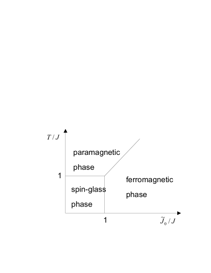
Figure 1: Phase diagram of the matter (e.g. quantum dot) subsystem within a multi-qubit-cavity such as a disordered quantum dot array coupled to an optical cavity mode. The scaled parameter $\tilde{J}_{0}$ can be varied simply by changing the qubit-cavity coupling strength $\lambda$ (see text). $T$ is the temperature.

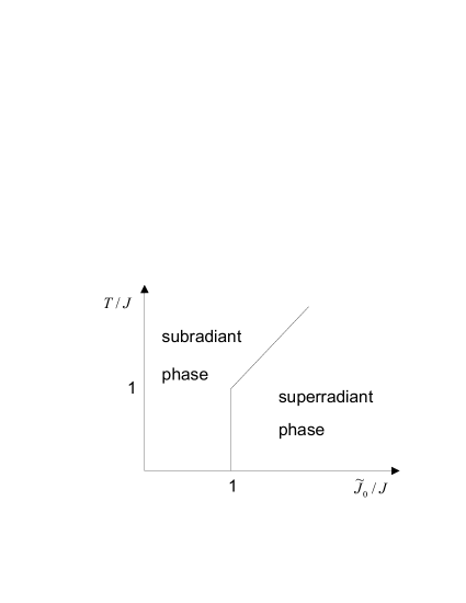
Figure 2: Phase diagram showing the superradiant-subradiant transition in the optical subsystem. In the absence of spin-spin interactions, the system is always superradiant due to the two-level system’s negligible energy gap $\epsilon$.

We now turn to consider the superradiant and subradiant photon states in the optical subsystem. We recall that the order parameter for the subradiant-superradiant phase separation is defined to be [14]:

$$\theta\equiv\left\langle\frac{a^{\dagger}a}{N}\right\rangle$$ (7)

In view of this, we insert a factor $h$ in the exponent $-\beta|\alpha|^{2}$ in $Z$, i.e.,

$$Z=\int\frac{d^{2}\alpha}{\pi}e^{-h\beta|\alpha|^{2}}{\rm Tr}e^{-\beta H^{\prime}}$$ (8)

so that

$$\theta=\left.\frac{1}{N}\frac{\partial[F]}{\partial h}\right|_{h=1}\ .$$ (9)

We now integrate out $\alpha$ in $Z$ and we obtain:

$$Z=\frac{1}{\beta}{\rm Tr}\exp\left\{-\beta\sum_{i<j}\left(-J_{ij}-\underline{\frac{2\lambda^{2}}{hN}}\right)\sigma^{X}_{i}\sigma^{X}_{j}+\beta\lambda^{2}\right\}\ .$$ (10)

Namely, the only modification is the extra $h$ in the denominator in the underlined term.

We now recall the definition of the free energy for spin glass systems [10, 20]:

$$[F]=-\frac{1}{\beta}[\log Z]=-\frac{1}{\beta}\int d[J]P(J_{ij})\log Z$$ (11)

where $d[J]=\prod_{ij}dJ_{ij}$ and we employ the replica method to approximate $[\log Z]$ as $\lim_{n\rightarrow 0}\frac{[Z^{n}]-1}{n}$. Going through the standard procedure of integrating out the quenched disorder in $J$s [20], we obtain:

$$[Z^{n}]=e^{N\beta^{2}J^{2}n/4}\int d[q]d[m]e^{\Omega}$$ (12)

where $d[q]\equiv\prod_{u<v}dq_{uv}$, $d[m]\equiv\prod_{u}dm_{u}$ and

$$\Omega = -\frac{N\beta^{2}J^{2}}{2}\sum_{u\neq v}q_{uv}^{2}-\frac{N\beta\tilde{J}_{0}}{2}\sum_{u}m_{u}^{2}$$ (13)

$$+\frac{N\beta^{2}J^{2}n}{4}+N\log{\rm Tr}e^{L}$$

with

$$L=\beta^{2}J^{2}\sum_{u<v}q_{uv}\sigma^{u}\sigma^{v}+\beta\sum_{u}\tilde{J}_{0}m_{u}\sigma^{u}$$ (14)

where $u,v$ are the replica indices and the $X$-superscripts in the $\sigma$s are dropped for clarity. Note that $\tilde{J_{0}}$ is now $(J_{0}+2\lambda^{2}/h)$ and so we obtain for $\partial[Z^{n}]/\partial h$ the following expression:

$$e^{N\beta^{2}J^{2}n/4}\times$$

$$\int d[q]d[m]\left\{\frac{2N\beta\lambda^{2}}{h^{2}}\sum_{u}(-m_{u}+2\langle\sigma^{u}\rangle_{L})m_{u}\right\}e^{\Omega}$$ (15)

where $\langle\sigma^{u}\rangle_{L}\equiv\frac{{\rm Tr}\sigma^{u}e^{L}}{{\rm Tr}e^{L}}$. It follows that

$$\theta = \left.\frac{1}{N}\frac{\partial[F]}{\partial h}\right|_{h=1}=\left.-\frac{1}{n\beta N}\frac{\partial[Z^{n}]}{\partial h}\right|_{h=1}$$ (16)

$$= \frac{2\lambda^{2}}{n}e^{N\beta^{2}J^{2}n/4}\times$$

$$\int d[q]d[m]\left\{\sum_{u}(2\langle\sigma^{u}\rangle_{L}-m_{u})m_{u}\right\}e^{\Omega}\ .$$

Since $\Omega$ is proportional to $N$, we can evaluate the integral by steepest-descent. In the thermodynamic limit $N\rightarrow\infty$, we find that

$$\theta={\rm const.}\times\frac{1}{n}\sum_{u}(2\langle\sigma^{u}\rangle_{L}-m_{u})m_{u}e^{\Omega_{\rm max}}\ \ .$$ (17)

Since $\Omega$ is optimized when

$$q_{uv}=\frac{1}{\beta^{2}J^{2}}\frac{\partial}{\partial q_{uv}}\log{\rm Tr}e^{L}\ =\ \langle\sigma^{u}\sigma^{v}\rangle_{L}$$ (18)

and

$$m_{u}=\frac{1}{\beta\tilde{J}_{0}}\frac{\partial}{\partial m_{u}}\log{\rm Tr}e^{L}\ =\ \langle\sigma^{u}\rangle_{L}\ \ ,$$ (19)

we have $\theta\propto\frac{1}{n}\sum_{u}m_{u}^{2}$. Therefore, in the replica-symmetric case, $\theta\propto m^{2}$ and one can then derive the superradiant-subradiant phase diagram as shown in Fig. 2, outlining the region where $m\neq 0$. Finally we note, by observation of Eq. (7), that spin-glass behaviour can also arise in a multi-qubit-cavity system with disorder in both $\{\lambda\}$ and $\{J\}$, as long as some of the $J$’s are negative.

In conclusion, we have analyzed a novel optical realization of a Hamiltonian system which is of great interest within the condensed matter community, and have deduced analytically the corresponding phase diagrams. In contrast to traditional realisations using magnetic solids, the phase transitions in this system can be explored simply by changing the matter-radiation coupling strength.

- [1] Scully M. O. and Zubairy M. S., Quantum Optics (Cambridge University Press, Cambridge) 1997; Hagley E. et al., Phys. Rev. Lett. 79 (1997) 1; Rauschenbeutel A. et al., Science 288 (2000) 2024; Dutra S. M., Knight P. L. and Moya-Cessa H., Phys. Rev. A 49 (1994) 1993; Young D. K., Zhang L., Awschalom D. D. and Hu E. L., Phys. Rev. B 66 (2002) 081307(R); Solomon G. S., Pelton M. and Yamamoto Y., Phys. Rev. Lett. 86 (2001) 3903; Moller B., Artemyev M. V., Woggon U. and Wannemacher R., Appl. Phys. Lett. 80 (2002) 3253; Berglund A. J., Doherty A. C. and Mabuchi H., Phys. Rev. Lett. 89 (2002) 068101.
- [2] Michler P., Single Quantum Dots: Fundamentals, Applications and New Concepts (Springer-Verlag, Berlin) 2003; Haug H. and Koch S. W., Quantum theory of the optical and electronic properties of semiconductors (World Scientific, singapore) 2004; Johnson N. F., J. Phys.: Condens. Matter 7 (1995) 965.
- [3] Nielsen M. A. and Chuang I. L., Quantum Computation and Quantum Information (Cambridge University Press, Cambridge) 2002; Quiroga L. and Johnson N. F., Phys. Rev. Lett. 83 ( 1999) 2270; Reina J. H., Quiroga L. and Johnson N. F., Phys. Rev. A 62 (2000) 012305.
- [4] Yoshie T. et al., Nature 432 (2004) 200; Wallraff A. et al., Nature 431 162; Guth hrlein G. R. et al., Nature 414 49; Imamoglu A. et al., Phys. Rev. Lett. 83 (1999) 4204.
- [5] Kiraz A et al., J. Optics B 5 (2003) 129.
- [6] Olaya-Castro A. and Johnson N. F., Handbook of Theoretical and Computational Nanotechnology, edited by Rieth M. and Schommers W. (American Scientific Publishers, New York) 2004 [Preprints: quant-ph/0406133].
- [7] Johnson S. G. and Joannopoulos J. D., Photonic Crystals: The Road from Theory to Practice (Kluwer, New York) 2001; Hui P. M. and Johnson N. F., Solid State Physics, edited by Ehrenreich H. and Spaepen F., Vol. 49 ed (Academic Press, New York) 1995.
- [8] Sakoglu U. et al., J. Optics B 21 (2004) 7.
- [9] Edwards S. F. and Anderson P. W., J. Phys. F 5 (1975) 965.
- [10] Sherrington D. and Kirkpatrick S., Phys. Rev. Lett. 35 (1975) 1792.
- [11] Loss D. and DiVincenzo D. P., Phys. Rev. A 57 (1998) 120; Elzerman J. M. et al., Nature 430 (2004) 431.
- [12] Dicke R. H. Phys. Rev. 170 (1954) 379.
- [13] Reslen J., Quiroga L. and Johnson N. F., Europhys. Lett. 69 (2005) 8; Lambert N., Emary C. and Brandes T., Phys. Rev. Lett. 92 (2004) 073602; Brandes T., Phys. Rep. 408 (2005) 315. Emary C. and Brandes T., Phys. Rev. Lett. 90 (2003) 044101; Lee C. F. and Johnson N. F., Phys. Rev. Lett. 93 (2004) 083001; Dusuel S. and Vidal J., Phys. Rev. Lett. 93 (2004) 237204.
- [14] Hepp K. and Lieb E. H., Ann. Phys. (N.Y.) 76 (1973) 360; Wang Y. K. and Hioe F. T., Phys. Rev. A 7 (1973) 831; Hioe F. T., Phys. Rev. A 8 (1973) 1440.
- [15] Rza̧żewski K. et al., Phys. Rev. Lett. 35 (1975) 432; Knight J. M. et al., Phys. Rev. A 17 (1978) 1454; Sung C. C. and Bowden C. M., J. Phys. A 12 (1979) 2273; Rza̧żewski K. and Wódkiewicz K., Phys. Rev. A 43 (1991) 593.
- [16] Keeling J., J. Phys.: Condens. Matter 19 (2007) 295213.
- [17] Jarret T. C., Lee C. F. and Johnson N. F., Phys. Rev. B 74 (2006) 121301(R).
- [18] Suzuki M., Prog. Theor. Phys. 56 (1976) 1454; Thirumalai D., Li Q. and Kirkpatrick T. R., J. Phys. A 22 (1989) 3339; Goldschmidt Y. Y. and Lai P. Y., Phys. Rev. Lett. 64 (1990) 2467.
- [19] Glauber R. J., Phys. Rev. 131 (1963) 2766.
- [20] Mezard M., Parisi G. and Virasoro M. A., Spin Glass Theory and Beyond (World Scientific, Singapore) 1987; Nishimori H., Statistical Physics of Spin Glasses and Information Processing (Oxford University Press, Oxford) 2001.