Quantum optical time-of-arrival model in three dimensions

Abstract

We investigate the three-dimensional formulation of a recently proposed operational arrival-time model. It is shown that within typical conditions for optical transitions the results of the simple one-dimensional version are generally valid. Differences that may occur are consequences of Doppler and momentum-transfer effects. Ways to minimize these are discussed.

1 Introduction

In quantum mechanics, as opposed to classical physics, the meaning of arrival time of a particle at a given location is not evident when the finite extent of the wave function and its spreading become relevant, such as for cooled atoms dropping out of a trap. Moreover, in the quantum case one will expect an arrival-time distribution, and there are different theoretical proposals for it, see e.g. [1, 2, 3, 4, 5, 6, 7, 8, 9, 10, 11, 12], the review in [13], and the book [14]. These arrival-time distributions have been controversially discussed in the literature since they are derived through purely theoretical arguments rather than operationally, i.e. without specifying a measurement procedure. But from the experimental point of view this is of course very important.

How then to measure the arrival time of a single quantum mechanical particle at a given location when the extent of its wave function becomes important? Here one has to distinguish between first arrival and repeated arrivals as in the case of a pendulum. For the former, the measurement procedure has to ensure that the arrival is indeed the first, not the second or third, i.e. that the particle did not already arrive before. This implies a sort of continuous or rapidly repeated observation of the same single particle in question. Doing the experiment again and again with many identically prepared particles will then give an arrival-time distribution.

To capture these requirements in a model it was suggested in [15] to consider a particle (“atom”) with two internal levels, which are connected by an optical transition, and to illuminate the arrival region by a laser. When the wave function of the particle enters the region the laser will populate the upper level and one can watch for the first spontaneous photon. The detection time of this photon can then be taken as the first arrival time in this region, at least approximately.

The model contains of course simplifying idealizations, which are indeed quite essential for extracting useful information. In general a measurement model should be flexible enough to capture the essence of the experiment and still provide, hopefully, close links with the schema of fundamental theory. That the fluorescence-based model is of such kind has been already demonstrated: the limits or operations by which theoretical time-of-arrival distributions, such as the flux or current density and Kijowski’s distribution, can be obtained by measurement have been determined [15, 16]. For other applications or extensions of the model see [17, 18, 19, 20, 21]. It should not be surprising that the conditions required for these “perfect measurements” may be rather extreme, or complicated to realize. The important point is that at least one knows what should be done, and one can reasonably understand and try to minimize the deviations from the ideal results.

A very basic simplifying assumption of all applications of the model so far has been the restriction of the atomic motion to one dimension (1D), associated with the $x$ axis hereafter, perpendicular to the laser (traveling wave) direction $y$. This approximation could in principle be badly wrong because of transversal velocity components in the incident atomic wave function or because of momentum transfer from the laser.

The aim of this paper is to generalize the fluorescence model to an arbitrary three dimensional wave packet impinging on a plane ($x=0$) which separates a laser-illuminated region ($x>0$) from a non-illuminated region ($x<0$). It will be shown that possible deviations from the 1D model can be attributed to an additional detuning term which is of kinetic origin. This kinetic detuning consists of a Doppler term and a term which is due to a momentum transfer from the laser field to the atom. It will be seen that deviations of the time-of-arrival distribution from the 1D model can be ascribed to two effects. First, there is increased or decreased reflection for blue or red kinetic detuning, respectively and, second, there is a less efficient driving of the atomic transition for both signs of the kinetic detuning which leads to a delay in the distribution. Numerical examples will be shown for two typical cases. For oblique incidence the kinetic effects can be compensated by appropriate laser detuning, whereas for a wave packet prepared with a very small width in laser direction this is not possible. The numerical results also show that the 1D model is valid over a wide range of parameters.

It will also be shown that the first photon distribution tends in some limit to the $x$ component of the total flux through the plane $x=0$, which is the natural generalization of a main result in [15].

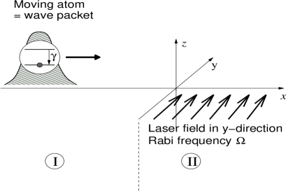
Figure 1: Schematic picture of the atom wave packet moving towards the laser-illuminated region.

2 The 3D model

As in [15] we consider a two-level atom which moves from the left towards the region $x>0$ which is illuminated by a traveling-wave laser directed parallel to the $y$ axis (see figure 1). The laser frequency may be on resonance or be detuned with respect to the atomic transition. We use the dipole and rotating wave approximations and employ the quantum jump approach [22, 23, 24]. In this approach the time development between two photon detections is given by a nonhermitean “conditional” Hamiltonian so that the norm of the wave function decreases; the norm squared at time $t$ just gives the probability for no photon detection until $t$. In a laser-adapted interaction picture (i.e. with $H_{0}=\hbar\omega_{\mathrm{L}}|2\rangle\langle 2|$) the conditional Hamiltonian becomes

$$H_{\mathrm{c}}=\frac{\hat{p}_{x}^{2}}{2m}+\frac{\hat{p}_{y}^{2}}{2m}+\frac{\hat{p}_{z}^{2}}{2m}+V(\hat{\mathbf{x}})$$ (1)

with

$$V(\hat{\mathbf{x}})=\frac{\hbar}{2}\Omega\theta(\hat{x})\left[\mathrm{e}^{\rmi k_{\mathrm{L}}\hat{y}}|2\rangle\langle 1|+\mathrm{e}^{-\rmi k_{\mathrm{L}}\hat{y}}|1\rangle\langle 2|\right]-\hbar\left(\Delta_{\mathrm{L}}+\rmi\gamma/2\right)|2\rangle\langle 2|,$$ (2)

where $\gamma$ is the decay (Einstein) constant of the excited state $|2\rangle$, $\Omega$ is the Rabi frequency, $\Delta_{\mathrm{L}}$ the detuning (laser angular frequency minus atomic-transition angular frequency), $k_{\mathrm{L}}$ the laser wavenumber, and $\theta$ the Heaviside function. The hats on positions and momenta ($\hat{\bf{x}},\hat{x},\hat{y},...,\hat{p}_{x},...$) denote operators to be distinguished from the corresponding ordinary vectors or c-numbers. Boldface capital Greek letters will designate atomic two-component wave functions, with the components for excited and ground state denoted by superscripts.

The operational time-of-arrival distribution $\Pi(t)$ for an atomic ensemble represented by a given wave function is defined as the temporal distribution of the first photon detected for each atom, and this is just the rate of the decrease of probability of detecting no photon. Hence one has the general result

$$\Pi(t)=-\rmd||\mathbf{\Psi}(t)||^{2}/\rmd t~{}.$$ (3)

By means of the Schrödinger equation and the above form of $H_{\mathrm{c}}$ one easily finds for the two-level system

$$\Pi(t)=\gamma\int_{-\infty}^{\infty}\,\mathrm{d}^{2}\mathbf{x}|\Psi^{(2)}(\mathbf{x},t)|^{2}.$$ (4)

To calculate $\Pi$ it is useful and physically illuminating to first obtain the eigenstates of the conditional Hamiltonian,

$$H_{\mathrm{c}}\mathbf{\Phi}_{\mathbf{k}}=E_{\mathbf{k}}\mathbf{\Phi}_{\mathbf{k}}.$$ (5)

Since $V(\hat{\mathbf{x}})$ does not depend on $\hat{z}$, the $z$ component of momentum is conserved so that there is free motion in $z$-direction and we only have to consider the two-dimensional motion in the $x$-$y$-plane. Therefore, from now on the position and momentum (wavenumber) vectors will always be two-dimensional.

Since the incident atoms are initially in the ground state and far from the laser region and are moving in the positive $x$-direction, we need the stationary scattering eigenstates which correspond to ground state plane waves coming in from the left. In matrix form, with $|1\rangle\equiv\textstyle{1\choose 0}$ and $|2\rangle\equiv\textstyle{0\choose 1}$, the (two-dimensional) conditional Hamiltonian can be written as

$$H_{\mathrm{c}}=\frac{\hat{p}_{x}^{2}}{2m}+\frac{\hat{p}_{y}^{2}}{2m}-\hbar(\Delta_{\mathrm{L}}+\rmi\gamma/2)\left(\begin{array}[]{cc}0&0\\ 0&1\end{array}\right)+\frac{\hbar}{2}\theta(\hat{x})\left(\begin{array}[]{cc}0&\Omega\mathrm{e}^{-\rmi k_{\mathrm{L}}\hat{y}}\\ \Omega\mathrm{e}^{\rmi k_{\mathrm{L}}\hat{y}}&0\end{array}\right)~{}.$$ (6)

For $x<0$ we use the ansatz

$$\mathbf{\Phi}_{\mathbf{k}}^{\mathrm{I}}(\mathbf{x})=\frac{1}{2\pi}\left(\begin{array}[]{c}\mathrm{e}^{\rmi\mathbf{k}\cdot\mathbf{x}}+R_{1}\mathrm{e}^{\rmi\mathbf{k}^{\prime}\cdot\mathbf{x}}\\ R_{2}\mathrm{e}^{\rmi\mathbf{q}\cdot\mathbf{x}}\end{array}\right)$$ (7)

with $(2\pi)^{-1}$ included for delta normalization in two-dimensional $\bf{k}$ space and with

$$E_{\mathbf{k}}=\frac{\hbar^{2}\mathbf{k}^{2}}{2m}=\frac{\hbar^{2}\mathbf{k}^{\prime 2}}{2m}\quad\mathrm{and}\quad\mathbf{q}^{2}=\mathbf{k}^{2}+\frac{m}{\hbar}(\rmi\gamma+2\Delta_{\mathrm{L}})~{}.$$ (8)

At this point the individual components of $\mathbf{k}^{\prime}$ and $\mathbf{q}$ are still unknown. They will be determined later from the matching conditions at $x=0$. For the region $x\geq 0$ we use, in analogy to the 1D model [15, 18], a plane wave ansatz of the form

$$\mathbf{\Phi}_{\mathbf{k}}^{\pm}(\mathbf{x})=\left(\begin{array}[]{c}1\\ \frac{2\lambda{{}_{\pm}}}{\Omega}\mathrm{e}^{\rmi k_{\mathrm{L}}y}\end{array}\right)\mathrm{e}^{\rmi\mathbf{k}^{\pm}\cdot\mathbf{x}}\equiv|E_{\pm}\rangle\mathrm{e}^{\rmi\mathbf{k}^{\pm}\cdot\mathbf{x}}$$ (9)

with as yet unknown $\lambda{{}_{\pm}}$ and $\mathbf{k}^{\pm}$. Inserting this into the eigenvalue equation (5) the exponential $\mathrm{e}^{\rmi\mathbf{k}^{\pm}\cdot\mathbf{x}}$ drops out and we get the matrix equation

$$\left(\begin{array}[]{cc}\frac{\hbar^{2}}{2m}\mathbf{k}^{\pm 2}&\frac{\hbar}{2}\Omega\mathrm{e}^{-\rmi k_{\mathrm{L}}y}\\ \frac{\hbar}{2}\Omega\mathrm{e}^{-\rmi k_{\mathrm{L}}y}&\frac{\hbar^{2}}{2m}\mathbf{k}^{\pm 2}-\hbar(\Delta+\rmi\gamma/2)\end{array}\right)|E_{\pm}\rangle=E_{\mathbf{k}}|E_{\pm}\rangle~{},$$ (10)

where

$$\Delta\equiv\Delta_{\mathrm{L}}-\frac{\hbar}{2m}(2k_{y}^{\pm}k_{\mathrm{L}}+k_{\mathrm{L}}^{2})$$ (11)

can be regarded as an effective detuning. We shall later analyze in detail the physical meaning of the second term, which is clearly of kinematic nature. Equation (10) is fulfilled if $\lambda_{\pm}$ and $\mathbf{k}^{\pm}$ satisfy

$$\lambda_{\pm}=-\frac{1}{4}\left(\rmi\gamma+2\Delta\right)\pm\frac{\rmi}{4}\sqrt{\left(\gamma-2\rmi\Delta\right)^{2}-4\Omega^{2}}$$ (12)

and

$$\mathbf{k}^{\pm 2}=\mathbf{k}^{2}-\frac{2m}{\hbar}\lambda_{\pm}~{}.$$ (13)

Note that $\lambda_{\pm}$ still contains the unknown components $k_{x}^{\pm}$ and $k_{y}^{\pm}$. The eigenstate for $x\geq 0$ is now a superposition of the form

$$\mathbf{\Phi}_{\mathbf{k}}^{\mathrm{II}}(\mathbf{x})=\frac{1}{2\pi}\left[C_{+}|E_{+}\rangle\mathrm{e}^{\rmi\mathbf{k}^{+}\cdot\mathbf{x}}+C_{-}|E_{-}\rangle\mathrm{e}^{\rmi\mathbf{k}^{-}\cdot\mathbf{x}}\right].$$ (14)

The coefficients $C_{\pm}$ will be determined from the matching conditions.

2.1 Matching Conditions

At $x=0$ the usual matching conditions, i.e.,

$$\eqalign{\mathbf{\Phi}_{\mathbf{k}}^{\mathrm{I}}(x=0,y)&=\mathbf{\Phi}_{\mathbf{k}}^{\mathrm{II}}(x=0,y)\\ \mathbf{\Phi}_{\mathbf{k}}^{\mathrm{I}\,^{\prime}}(x=0,y)&=\mathbf{\Phi}_{\mathbf{k}}^{\mathrm{II}\,^{\prime}}(x=0,y)}$$ (15)

are imposed. This yields the equations

$$\mathrm{e}^{\rmi k_{y}y}+R_{1}\mathrm{e}^{\rmi k_{y}^{\prime}y}=C_{+}\mathrm{e}^{\rmi k_{y}^{+}y}+C_{-}\mathrm{e}^{\rmi k_{y}^{-}y}$$ (16a)

$$R_{2}\mathrm{e}^{\rmi q_{y}y}=\frac{2\lambda_{+}}{\Omega}C_{+}\mathrm{e}^{\rmi(k_{\mathrm{L}}+k_{y}^{+})y}+\frac{2\lambda_{-}}{\Omega}C_{-}\mathrm{e}^{\rmi(k_{\mathrm{L}}+k_{y}^{-})y}$$ (16b)

$$\mathbf{k}\mathrm{e}^{\rmi k_{y}y}+\mathbf{k}^{\prime}R_{1}\mathrm{e}^{\rmi k_{y}^{\prime}y}=\mathbf{k}^{+}C_{+}\mathrm{e}^{\rmi k_{y}^{+}y}+\mathbf{k}^{-}C_{-}\mathrm{e}^{\rmi k_{y}^{-}y}$$ (16c)

$$\mathbf{q}R_{2}\mathrm{e}^{\rmi q_{y}y}=\mathbf{k}^{+}\frac{2\lambda_{+}}{\Omega}C_{+}\mathrm{e}^{\rmi(k_{\mathrm{L}}+k_{y}^{+})y}+\mathbf{k}^{-}\frac{2\lambda_{-}}{\Omega}C_{-}\mathrm{e}^{\rmi(k_{\mathrm{L}}+k_{y}^{-})y}$$ (16d)

As (16a) has to hold for all $y$ one obtains

$$k_{y}=k_{y}^{\prime}=k_{y}^{+}=k_{y}^{-}~{},$$ (16q)

and with this one finds from (8) for $k_{x}^{\prime}$ of the reflected component

$$k_{x}^{\prime}=-k_{x}.$$

From (16q) it follows that $\Delta$ is independent of $\mathbf{k}^{\pm}$, and consequences of this will be discussed in more detail in the next subsection. For the $x$ components of the wave vector inside the laser region one then obtains

$$k_{x}^{\pm 2}=k_{x}^{2}+\frac{m}{2\hbar}\left(\rmi\gamma+2\Delta\right)\mp\frac{\rmi m}{2\hbar}\sqrt{\left(\gamma-2\rmi\Delta\right)^{2}-4\Omega^{2}},$$

and $k_{x}^{\pm}$ are given by the roots of this with positive imaginary part so that the wave decays in the laser region. Both depend on $k_{y}$ through the effective detuning $\Delta$. From (16b) one gets by a similar argument

$$q_{y}=k_{y}+k_{\mathrm{L}},$$

where $\hbar k_{\mathrm{L}}$ is the momentum transfer from the laser field to the excited state of the atom. This and (8) in turn lead to

$$q_{x}^{2}=k_{x}^{2}+\frac{m}{\hbar}\left(\rmi\gamma+2\Delta\right)$$

for the reflected part of the excited state, and $q_{x}$ is obtained by again taking the root with positive imaginary part so that the excited wave decays at long distances from the laser. With these simplifications the matching conditions (16) now take the form

$$1+R_{1}=C_{+}+C_{-}$$ (16ra)

$$R_{2}=\frac{2\lambda_{+}}{\Omega}C_{+}+\frac{2\lambda_{-}}{\Omega}C_{-}$$ (16rb)

$$k_{x}(1-R_{1})=k_{x}^{+}C_{+}+{k}_{x}^{-}C_{-}$$ (16rc)

$$q_{x}R_{2}=k_{x}^{+}\frac{2\lambda_{+}}{\Omega}C_{+}+k_{x}^{-}\frac{2\lambda_{-}}{\Omega}C_{-}$$ (16rd)

which look formally just same as in the 1D case, only with $k^{\pm}$ and $q$ replaced by $k^{\pm}_{x}$ and $q_{x}$ and with $\lambda_{\pm}$ defined as in (12). Accordingly the coefficients $R_{1}$, $R_{2}$, $C_{\pm}$ have the same form as in the 1D model,

$$C_{+}=-2k_{x}(q_{x}+k_{x}^{-})\lambda_{-}/D$$ (16rsa)

$$C_{-}=2k_{x}(q_{x}+k_{x}^{+})\lambda_{+}/D$$ (16rsb)

$$R_{2}=k_{x}(k_{x}^{-}-k_{x}^{+})\Omega/D$$ (16rsc)

$$R_{1}=[\lambda_{+}(q_{x}+k_{x}^{+})(k_{x}-k_{x}^{-})-\lambda_{-}(q_{x}+k_{x}^{-})(k_{x}-k_{x}^{+})]/D$$ (16rsd)

and

$$D=\lambda_{+}(k_{x}+k_{x}^{-})(q_{x}+k_{x}^{+})-\lambda_{-}(k_{x}+k_{x}^{+})(q_{x}+k_{x}^{-}).$$ (16rse)

Finally, taking into account the matching conditions, (7) and (14) take the form

$$\mathbf{\Phi}_{\mathbf{k}}^{\mathrm{I}}(\mathbf{x})=\frac{1}{2\pi}\left(\begin{array}[]{c}\left[\mathrm{e}^{\rmi k_{x}x}+R_{1}\mathrm{e}^{-\rmi k_{x}x}\right]\mathrm{e}^{\rmi k_{y}y}\\ R_{2}\mathrm{e}^{-\rmi q_{x}x}\mathrm{e}^{\rmi(k_{y}+k_{\mathrm{L}})y}\end{array}\right)$$ (16rst)

for $x<0$ and

$$\mathbf{\Phi}_{\mathbf{k}}^{\mathrm{II}}(\mathbf{x})=\frac{1}{2\pi}\left[C_{+}\left(\begin{array}[]{c}1\\ \frac{2\lambda_{+}}{\Omega}\mathrm{e}^{\rmi k_{\mathrm{L}}y}\end{array}\right)\mathrm{e}^{\rmi k_{x}^{+}x}+C_{-}\left(\begin{array}[]{c}1\\ \frac{2\lambda_{-}}{\Omega}\mathrm{e}^{\rmi k_{\mathrm{L}}y}\end{array}\right)\mathrm{e}^{\rmi k_{x}^{-}x}\right]\mathrm{e}^{\rmi k_{y}y}$$ (16rsu)

for $x>0$.

2.2 Effective detuning: Doppler shift and momentum transfer

Using (16q), the effective detuning (11) can be written as

$$\Delta=\Delta_{\mathrm{L}}-\Delta_{\mathrm{K}},$$ (16rsv)

with the kinetic detuning

$$\Delta_{\mathrm{K}}\equiv\frac{\hbar}{2m}(2k_{y}k_{\mathrm{L}}+k_{\mathrm{L}}^{2})=\frac{\hbar}{2m}(k_{y}+k_{\mathrm{L}})^{2}-\frac{\hbar}{2m}k_{y}^{2}$$

so that $\hbar\Delta_{\mathrm{K}}$ is the $y$ momentum component contribution to the kinetic energy difference between ground state and excited state, as seen from the terms $k_{y}$ and $k_{y}+k_{\mathrm{L}}$ in the plane wave exponents in (16rst) and (16rsu). We may also express $\Delta_{\mathrm{K}}$ in terms of the speed of light in vacuum $c$, the laser angular frequency $\omega_{\mathrm{L}}=k_{\mathrm{L}}c$, the $y$ component of the incident velocity $v_{y}=\hbar k_{y}/m$, and of a velocity $v_{\mathrm{R}}\equiv\hbar k_{\mathrm{L}}/m$, namely

$$\Delta_{\mathrm{K}}=\frac{\omega_{\mathrm{L}}}{c}\left(v_{y}+\frac{v_{\mathrm{R}}}{2}\right).$$ (16rsw)

The form of (16rsw) can also be derived by classically modeling the resonance condition with simple energy and momentum conservation arguments. To see this we rewrite it as

$$\Delta_{\mathrm{K}}=\omega_{\mathrm{D}}+\omega_{\mathrm{R}}$$ (16rsx)

with $\omega_{\mathrm{D}}\equiv\omega_{\mathrm{L}}v_{y}/c$ and $\omega_{\mathrm{R}}\equiv\hbar k_{\mathrm{L}}^{2}/2m=\omega_{\mathrm{L}}v_{\mathrm{R}}/2c$. The first term is the ordinary Doppler shift due to the incident velocity component $v_{y}$ and the second can be viewed as a frequency shift caused by the change of the atomic kinetic energy due to the absorption of a laser photon. Recall that the momentum transfer from the laser is only directed along the $y$ direction. It is interesting to note that the kinetic detuning in (16rsx) has in fact already the form of a Doppler shift formula with the role of the velocity played by the average of the velocity components for ground state and excited state along the direction of the laser. Indeed, for fixed non-zero values of $k_{y}$ and $k_{\mathrm{L}}$ in a stationary wave the two effects cannot be disentangled and act simultaneously in the form of a single kinetic detuning. It is, however, possible to distinguish their consequences for wave packets, as discussed below, since $k_{\mathrm{L}}$ is fixed by the laser wavelength, whereas $k_{y}$ varies for each incident atomic momentum component, or by sweeping over the incidence angle.

Note also the signs in the effective total detuning (16rsv): a large, positive, kinetic detuning (energy transfer) implies a red shift whereas a large laser, positive detuning amounts to a blue shift. They may compensate each other, as we shall illustrate afterwards, while $\omega_{\mathrm{D}}$ and $\omega_{\mathrm{R}}$ may also cancel each other for a negative velocity $v_{y}$ opposed to the laser beam.

3 The First-Photon Distribution

Until detection of the first photon, the conditional time development of a wave packet $\mathbf{\Psi}(\mathbf{x},t)$ corresponding to a particle in the internal ground state coming in from the left can now be written as in the 1D case in terms of the plane-wave solutions,

$$\mathbf{\Psi}(\mathbf{x},t)=\int_{0}^{\infty}\!\mathrm{d}k_{x}\,\!\int_{-\infty}^{\infty}\!\mathrm{d}k_{y}\,\tilde{\psi}(\mathbf{k})\mathbf{\Phi_{\mathbf{k}}}(\mathbf{x})\mathrm{e}^{-\rmi\hbar\mathbf{k}^{2}t/2m},$$ (16rsy)

where $\tilde{\psi}(\mathbf{k})$ is the momentum amplitude the wave packet would have as a freely moving particle at $t=0$. Inserting this into (4) one obtains the first-photon distribution. This gives a six-dimensional integral of which the $x$, $y$, and $k_{y}^{\prime}$ integrations can be carried out analytically, yielding

$$\Pi(t)=\frac{\gamma}{2\pi}\int_{0}^{\infty}\!\!\!\mathrm{d}k_{x}\,\!\!\int_{0}^{\infty}\!\!\!\mathrm{d}k_{x}^{\prime}\,\!\!\int_{-\infty}^{\infty}\!\!\!\mathrm{d}k_{y}\,\overline{\widetilde{\psi}(k_{x},k_{y})}\widetilde{\psi}(k_{x}^{\prime},k_{y})\left[\frac{\rmi\overline{R_{2}}R_{2}^{\prime}}{q_{x}^{\prime}-\overline{q}_{x}}+\rmi\frac{4\overline{C_{+}}C_{+}^{\prime}\overline{\lambda}_{+}\lambda_{+}^{\prime}}{\Omega^{2}(k_{x}^{+\prime}-\overline{k_{x}^{+}})}\right.$$ (16rsz)

$$\left.{}+\rmi\frac{4\overline{C_{+}}C_{-}^{\prime}\overline{\lambda}_{+}\lambda_{-}^{\prime}}{\Omega^{2}(k_{x}^{-\prime}-\overline{k_{x}^{+}})}+\rmi\frac{4\overline{C_{-}}C_{+}^{\prime}\overline{\lambda}_{-}\lambda_{+}^{\prime}}{\Omega^{2}(k_{x}^{+\prime}-\overline{k_{x}^{-}})}+\rmi\frac{4\overline{C_{-}}C_{-}^{\prime}\overline{\lambda}_{-}\lambda_{-}^{\prime}}{\Omega^{2}(k_{x}^{-\prime}-\overline{k_{x}^{-}})}\right]\mathrm{e}^{-\rmi\hbar(k_{x}^{\prime 2}-k_{x}^{2})t/2m}.$$

This form of the first-photon distribution will be now used to numerically look for deviations from the 1D results in different parameter regimes.

The relevance of possible deviations can be estimated by comparing the two-dimensional (2D) eigenstates with those of the 1D model which are given by [15, 18]

$$\mathbf{\Phi}^{\mathrm{(1D)}}_{{k}}({x})=\cases{\frac{1}{\sqrt{2\pi}}\left(\begin{array}[]{c}\mathrm{e}^{\rmi kx}+R_{1}\mathrm{e}^{-\rmi kx}\\ R_{2}\mathrm{e}^{-\rmi qx}\end{array}\right)&for $x<0$\\ \frac{1}{\sqrt{2\pi}}\left[C_{+}\left(\begin{array}[]{c}1\\ \frac{2\lambda_{+}^{\mathrm{(1D)}}}{\Omega}\end{array}\right)\mathrm{e}^{\rmi k_{+}x}+C_{-}\left(\begin{array}[]{c}1\\ \frac{2\lambda_{-}^{\mathrm{(1D)}}}{\Omega}\end{array}\right)\mathrm{e}^{\rmi k_{-}x}\right]&for $x\geq 0$}$$ (16rsaa)

where

$$q=\sqrt{k^{2}+\frac{2m}{\hbar}(\Delta_{\mathrm{L}}+\rmi\gamma/2)}~{},\quad k_{\pm}=k^{2}-\frac{2m}{\hbar}\lambda_{\pm}~{},$$

$$\lambda_{\pm}=-\frac{1}{4}\left(\rmi\gamma+2\Delta_{\mathrm{L}}\right)\pm\frac{\rmi}{4}\sqrt{(\gamma-2\rmi\Delta_{\mathrm{L}})^{2}-4\Omega^{2}}$$

and roots are taken with positive imaginary parts. One can go from 2D to 1D formulas ($q_{x}\rightarrow q$, $\lambda^{(\mathrm{2D})}_{\pm}\rightarrow\lambda^{(\mathrm{1D})}_{\pm}$, $k^{\pm}_{x}\rightarrow k_{\pm}$) simply by dropping the kinetic detuning $\Delta_{\mathrm{K}}$, which is thus identified as the physical reason for possible deviations from the 1D results.

For optical transitions, typical values of $\Omega$, $\gamma$ or $\Delta_{\mathrm{L}}$ are of order $10^{7}$ s^-1, while the shift $\omega_{\mathrm{R}}$ in (16rsw) for Cs is of order $10^{5}$ s^-1. For perpendicular incidence, i.e. $\langle k_{y}\rangle=0$, and for velocities $v_{y}$ corresponding to a $\Delta_{y}=1\mu$m wave packet, the Doppler shift $\omega_{\mathrm{D}}$ is even smaller, namely of order $10^{3}$ s^-1. So the 1D model results may be expected to hold quite generally in a broad (ordinary) range of parameters. The number of parameters is rather large so a full systematic analysis of all possible cases in the vast parameter space is out of the question. Nevertheless, it is worth examining the convergence from 2D to 1D results in some typical cases. Since the laser and kinetic detunings, $\Delta_{\mathrm{L}}$ and $\Delta_{\mathrm{K}}$, are always combined together in $\lambda_{\pm}$, $k_{x}^{\pm}$ and $q$, one possible limit for pure 1D behaviour is $|\Delta_{\mathrm{L}}|\gg|\Delta_{\mathrm{K}}|$. Moreover, from (16rsv) it is also possible to find 1D results if the two contributions to the effective detuning cancel each other, i.e. if $\Delta_{\mathrm{L}}=\Delta_{\mathrm{K}}$, as we shall discuss below. $\Delta_{\mathrm{K}}$ may also be zero because of a cancellation between Doppler and momentum-transfer shifts in oblique incidence. One may similarly reduce the equations to 1D if $\Omega$ or $\gamma$ are large with respect to all other frequency parameters. For strong driving, $\Omega\gg\gamma,\Delta_{\mathrm{L}}$, more detailed sufficient conditions would be $k_{y}\ll k_{x}^{2}/k_{\mathrm{L}}$, $k_{y},k_{\mathrm{L}}\ll\frac{m}{\hbar}\Omega/k_{\mathrm{L}}$, and $k_{\mathrm{L}}^{2}\ll k_{x}^{2}$. This means that a two-dimensional wave packet, with given mean momenta $\langle k_{x}\rangle$, $\langle k_{y}\rangle$ and momentum widths $\Delta_{k_{x}}$, $\Delta_{k_{y}}$, can be described by the 1D model if it has only small $k_{y}$ components and if at the same time $k_{\mathrm{L}}$ is small compared to the $k_{x}$ component and $\Delta_{\mathrm{K}}\ll\Omega$. In particular the momentum spread of the wave-packet in $y$ direction should be small compared to the momentum spread in $x$ direction. This, on the other hand, corresponds to a large width $\Delta_{y}$ in real space which is very satisfactory since for $\Delta_{y}\rightarrow\infty$ the two-dimensional wave packet tends to a one dimensional one.

This behaviour can be seen in figure 2 for arrival time distributions of minimum-uncertainty product Gaussian wave packets with different widths $\Delta_{y}$ and fixed width $\Delta_{x}$ at the preparation time $t=0$ (see the caption for details), where parameters of Cs have been used. For large widths $\Delta_{y}$ the time of arrival distribution is identical to the one which is obtained from a one-dimensional Gaussian wave packet of width $\Delta_{x}$ in the 1D model. For very small widths $\Delta_{y}$ first a slight enhancement in the height of the distribution and then a delay in the form of an enhanced tail of the distribution can be seen.

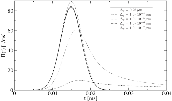
Figure 2: Arrival time density for a caesium atom with the parameters $\Omega=1.67\cdot 10^{8}\,\mathrm{s}^{-1}$, $\gamma=3.3\cdot 10^{8}\,\mathrm{s}^{-1}$, prepared at $t=0$ as a minimum-uncertainty product Gaussian wave packet with $\Delta_{x}=0.24\cdot 10^{-6}\,\mathrm{m}$, $\langle k_{x}\rangle=0$, and with initial average position $\langle x_{0}\rangle=-1.32\cdot 10^{-6}\,\mathrm{m}$, and velocity $\langle v_{0}\rangle=9\,\mathrm{cm/s}$. The solid line distribution coincides with the 1D distribution.

The physical reasons for these two effects are a dependence of the reflection coefficient on the velocity in $y$ direction and the Doppler effect, respectively, as will be explained in the next paragraph. It is seen in figure 2 that a significant deviation from the 1D distribution occurs for the Cs parameters used here if the wave packet is prepared with a width at least three orders of magnitude smaller in $y$ direction than in $x$ direction. A deviation from the 1D time of arrival can also be seen if a sufficiently large momentum $\langle k_{y}\rangle$ is chosen, which corresponds to oblique incidence of the atoms onto the laser region. Figure 3 shows numerical results for Cs wave packets with different positive average initial momenta. Again there are two effects: first an increase in height of the distribution and then for even larger momenta a delay. For negative initial average momenta (see figure 4) on the other hand one first sees a decrease in height of the distributions and then also a delay.

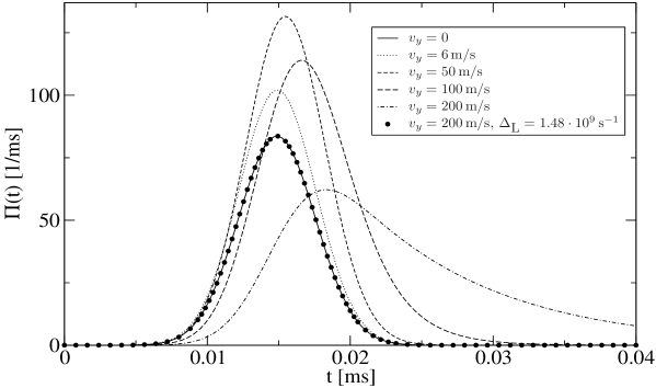
Figure 3: Arrival time density for Gaussian wave packets with different positive initial average velocities $\langle v_{y}\rangle$. Atomic parameters as in figure 2. The dotted graph shows a distribution with $\Delta_{\mathrm{L}}=\Delta_{\mathrm{K}}$ for compensation of the kinetic effects.

The change in height of the distributions is due to the $k_{y}$ dependence of the reflection coefficients, as will be explained now. Compared to the eigenstate with $k_{y}=0$ the eigenfunctions with positive $k_{y}$ have a smaller reflected part whereas the eigenfunctions with negative $k_{y}$ have a larger reflected part, as shown in figure 5. This behaviour can be understood via the dipole force and the effective detuning of (16rsv) as follows. Positive values of $k_{y}$ lead to an effective red detuning while negative values lead to blue detuning. Therefore states with positive $k_{y}$ are pushed into the laser region resulting in decreased reflection and states with negative $k_{y}$ are pulled out of the laser region resulting in increased reflection. The delay is due to the diminished efficiency of the laser because of the Doppler shift which also explains the decrease in reflection for very high negative momenta seen in figure 5. For the parameter values of Caesium used here one again has to insert rather extreme values of $\langle k_{y}\rangle$, i.e. at least three orders of magnitude larger than $\langle k_{x}\rangle$, to see deviations from the 1D distribution. The effects of nonzero initial average momentum $k_{y}$ can be compensated by choosing a laser detuning $\Delta_{\mathrm{L}}=\Delta_{\mathrm{K}}$ which leads to zero average effective detuning. Since quantum effects in the time-of-arrival can only be observed for sufficiently small incident velocities and since the 3D distribution corresponds to the 1D distribution with $v_{x}$ as incident velocity the oblique incidence could be useful in order to obtain broader distributions.

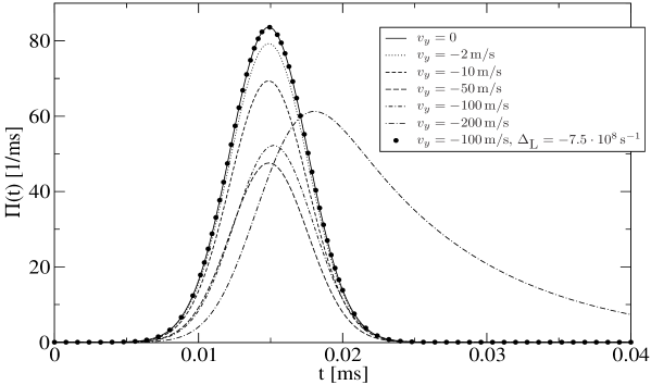
Figure 4: Arrival time distribution for wave packets with different negative initial average velocities $\langle v_{y}\rangle$. Atomic parameters as in figure 2. The dotted graph again shows a distribution with $\Delta_{\mathrm{L}}=\Delta_{\mathrm{K}}$ for compensation of the kinetic effects.

The effects of very small widths $\Delta_{y}$, seen in figure 2, can also be understood by means of the two effects explained above. The delay is again due to the Doppler effect. Indeed, since small uncertainty in position means large uncertainty in momentum, a wave packet prepared with small $\Delta_{y}$ will broaden very rapidly so that the tails of the wave packet move away from the center. Due to the Doppler effect these tails see a detuned laser and the wave packet as a whole is excited less efficiently. Since there is a shift with positive and negative sign for different components, it is not possible to compensate this effect by laser detuning. The increase in height of the distribution is a little bit subtler. Starting from $k_{y}=0$ the decrease of $|R_{1}|^{2}(k_{y})$ in figure 5 when going to positive values of $k_{y}$ is slightly steeper than the increase in the other direction. Therefore there is less reflection for increasing $\Delta_{k_{y}}$, although both positive and negative values of $k_{y}$ occur with the same weight in the wave packet.

Deviations from the 1D distribution also occur for a large shift $\omega_{\mathrm{R}}$, i.e. if $k_{\mathrm{L}}^{2}$ is large compared to the other relevant parameters. However, this requires an incident velocity smaller than the recoil velocity $v_{\mathrm{R}}$ and, for a laser transition in the optical range, a metastable transition with a lifetime of the order of one tenth of a second.

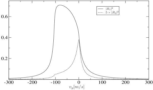
Figure 5: Plot of the modulus squared of the reflection coefficients $R_{1}$ and $R_{2}$ as a function of the incident velocity $v_{y}$. Parameter values as in figure 2. The graph of $|R_{2}|^{2}$ is stretched by a factor of 5.

4 Deconvolution

The operational model to quantum arrival times presented in [15] and generalized here to three dimensions shows that there may arise two potential problems when comparing operational with ideal distributions, namely reflection due to the laser field and detection delay. Reflection in the ground state means that no photon is emitted and hence the arrival of the atom is not detected. Delay is due to the fact that excitation and de-excitation of the atom take a finite time. If one tries to get rid of the delay by increasing both the decay rate $\gamma$ and the Rabi frequency $\Omega$ this will increase reflection in the ground state and thus lead to a detection decrease. To circumvent this one may try to use a gentle (i.e., not reflecting) weak excitation and then subtract the long delays in a suitable manner. In [15] this was done by a deconvolution with the first-photon distribution of an atom at rest as follows. It was assumed that the “experimental” time-of-arrival distribution $\Pi(t)$ is given by a convolution of a hypothetical ideal distribution $\Pi_{\mathrm{id}}$ with the (known) first-photon distribution $W(t)$ of a two-level atom at rest,

$$\Pi=\Pi_{\mathrm{id}}\star W.$$ (16rsab)

In the limit of large $\gamma$ it was then seen that the resulting ideal distribution tends to the quantum mechanical flux

$$\Pi_{\mathrm{id}}\rightarrow J_{\psi}=\frac{\hbar}{2m\rmi}\left\{\overline{\psi(0,t)}\psi^{\prime}(0,t)-\overline{\psi^{\prime}(0,t)}\psi(0,t)\right\}.$$

A similar calculation can be carried out here and it yields the $x$ component of the total flux through the plane $x=0$,

$$\Pi_{\mathrm{id}}\rightarrow\overline{J}_{x}(0,t)=\left[\int_{-\infty}^{\infty}\mathrm{d}y\,J_{x}(x,y,t)\right]_{x=0}$$

with

$$J_{x}(x,y,t)=\frac{\hbar}{2m\rmi}\left\{\overline{\psi(x,y,t)}\frac{\mathrm{d}\psi\,}{\mathrm{d}x\,}(x,y,t)-\overline{\frac{\mathrm{d}\psi\,}{\mathrm{d}x\,}(x,y,t)}\psi(x,y,t)\right\}.$$

This is the result one would expect as the natural generalization when carrying over the 1D case to three dimensions.

5 Conclusions

We have generalized the quantum optical time-of-arrival model of [15] to three dimensional space in order to describe a more realistic setup and verify the approximations made there. When considering arrivals at the plane $x=0$ we have seen that only $x$ and $y$ directions have to be considered, which leads to an effective 2D model. Deviations from the 1D model can be described via a kinetic detuning $\Delta_{\mathrm{K}}$ which consists of two terms for two distinct effects. One is a detuning of the atomic transition from the laser frequency due to the Doppler effect for velocity components $v_{y}$ in the laser direction. The other is the gain of momentum of the atom in the positive-$y$ (laser) direction by absorption of a laser photon. Again via the Doppler effect, this leads to a shift in frequency of the internal transition of the atom in the lab frame. A nonzero kinetic detuning in turn leads to two different effects affecting the time-of-arrival distribution. Blue and red detuning results in increased and decreased reflection, respectively, and therefore in a smaller or larger height of the distribution. At the same time both detunings lead to a less efficient driving of the atomic transition by the laser and thus to a delay in the distribution.

We have described typical situations for which deviations from the 1D model occur. One is the preparation of a wave packet with very small width $\Delta_{y}$. Then the corresponding large momentum width leads to large transversal velocity components. Another possibility is oblique incidence with large (positive or negative) mean transversal momentum $\langle k_{y}\rangle$. In the latter case the deviations can be compensated by an appropriate detuning of the laser whereas in the first case this is not possible. Inserting realistic atomic parameters it has been shown that over a wide range of parameters the 1D model is generally applicable.

A main theoretical result of reference [15] was that the first-photon distribution tends in some limit to the quantum mechanical probability current, opening the way towards a measurement of this quantity. A similar calculation in the generalized case gives the $x$ component of the total flux through the plane $x=0$, which is the natural generalization of the 1D result.

References

References

- [1] Allcock G R 1969 Ann. Phys. (N.Y.) 53 253; 53 286; 53 311
- [2] Kijowski J 1974 Rep. Math. Phys. 6 361
- [3] Werner R 1986 J. Math Phys. 27 793
- [4] Blanchard P and Jadczyk A 1996 Helv. Phys. Acta 69 613.
- [5] Giannitrapani R 1997 Int. J. Theor. Phys. 36 1575
- [6] Leavens C R 1998 Phys. Rev. A 58 840
- [7] Aharonov Y, Oppenheim J, Popescu S, Reznik B and Unruh W G 1998 Phys. Rev. A 57 4130
- [8] Halliwell J J 1999 Prog. Theor. Phys. 102 707
- [9] Kochański P and Wódkiewicz K 1999 Phys. Rev. A 60, 2689
- [10] León J, Julve J, Pitanga P and de Urríes F J 2000 Phys. Rev. A 61 062101
- [11] Galapon E A 2002 Proc. Roy. Soc. 458 451
- [12] Ruschhaupt A 2002 J. Phys. A: Math. Gen. 35 10429
- [13] Muga J G and Leavens C R 2000 Phys. Rep. 338 353
- [14] Muga J G, Sala R and Egusquiza I L 2002 (eds) Time in Quantum Mechanics (Berlin: Springer)
- [15] Damborenea J A, Egusquiza I L, Hegerfeldt G C and Muga J G 2002 Phys. Rev. A 66 052104
- [16] Hegerfeldt G C, Seidel D and Muga J G 2003 Phys. Rev. A 68 022111
- [17] Damborenea J A, Egusquiza I L, Hegerfeldt G C and Muga J G 2003 J. Phys. B: At. Mol. Opt. Phys. 36 2657
- [18] Navarro B, Egusquiza I L, Muga J G and Hegerfeldt G C 2003 Phys. Rev. A 67 063819
- [19] Navarro B, Egusquiza I L, Muga J G and Hegerfeldt G C 2003 J. Phys. B: At. Mol. Opt. Phys. 36 3899
- [20] Ruschhaupt A, Damborenea J A, Navarro B, Muga J G and Hegerfeldt G C 2004 Europhys. Lett. 67 1
- [21] Hegerfeldt G C, Seidel D, Muga J G and Navarro B 2004 Phys. Rev. A 70 012110
- [22] Hegerfeldt G C and Wilser T S 1992 in: Classical and Quantum Systems. Proceedings of the Second International Wigner Symposium 1991, edited by H. D. Doebner, W. Scherer, and F. Schroeck, (World Scientific, Singapore), p. 104; Hegerfeldt G C 1993 Phys. Rev. A 47 449
- [23] Dalibard J, Castin Y and Mølmer K 1992 Phys. Rev. Lett. 68 580
- [24] Carmichael H 1993 An Open Systems Approach to Quantum Optics (Berlin: Springer)