Quantum state reconstruction via continuous measurement

Abstract

We present a new procedure for quantum state reconstruction based on weak continuous measurement of an ensemble average. By applying controlled evolution to the initial state new information is continually mapped onto the measured observable. A Bayesian filter is then used to update the state-estimate in accordance with the measurement record. This generalizes the standard paradigm for quantum tomography based on strong, destructive measurements on separate ensembles. This approach to state estimation can be non-destructive and real-time, giving information about observables whose evolution cannot be described classically, opening the door to new types of quantum feedback control.

The control of quantum mechanical systems is finding new applications in information processing tasks such as cryptography and computation Nielsen2000 . Experimental reconstruction of a quantum state is thus essential to verify preparation, to detect the presence of errors due to noise and decoherence, and to determine the fidelity of control protocols using process tomography. Moreover, real-time “state estimation” may allow improvement of precision metrology beyond the standard quantum limit Geremia03 , with the possibility of active control through closed-loop feedback protocols Geremia04 . In addition, measurement of the quantum state can provide information about unknown or nontrivial dynamics, such as those arising in the study of quantum chaos. Laboratory demonstrations of state reconstruction are numerous and span a broad range of physical systems, including light fields smithey93 , molecules dunn95 , ions leibfried96 , atoms kurtsiefe97 , spins chuang98 ; Klose01 , and entangled photon pairs white99 .

In this letter we consider a new protocol for quantum state reconstruction based on continuous, weak measurement of a single observable on a single ensemble of identically prepared systems. The ensemble is driven so that each member undergoes an identical, carefully designed dynamical evolution that continually maps new information onto the measured quantity. This is in contrast to the standard paradigm for quantum state reconstruction based on strong and therefore destructive measurements, often of a large set of observables performed on many copies of the unknown state. Our weak measurement approach has a number of possible advantages in situations that lend themselves naturally to working with ensembles. Strong measurements on ensembles are inefficient because only a single observable can be measured after each preparation and the information gained about the observable is extracted independent of the required fidelity. By contrast, weak measurements can be optimized to obtain just enough information to estimate the density matrix to some required fidelity, in real time, and with minimal disturbance of each member. One can then imagine using the extracted information to perform closed-loop feedback control based on knowledge about the entire quantum state, rather than on conventional “state estimation” of Gaussian random variables that evolve according to classical dynamics, as considered to date Molmer04 . Our procedure is broadly applicable in systems where continuous weak measurement tools have been developed, such as nuclear magnetic resonance in molecules chuang98 and polarization spectroscopy in dilute atomic vapors Smith03 , but where noise and decoherence limits the ability to perform strong measurements regardless of the amount of signal averaging.

To perform quantum state reconstruction one considers a set of measurements $\{M^{(i)}\}$, each of which has a set of outcomes $m_{j}^{(i)}$, $\{j=1,2,\ldots,j^{(i)}_{\text{max}}\}$. The set is said to be “informationally complete” if for a given state $\rho_{0}$ the set of probabilities $\{p_{j}^{(i)}\}$ of the measurement outcomes can be inverted to determine $\rho_{0}$. In our protocol the probabilities are assigned using a single ensemble $\rho_{N}=\rho_{0}^{\otimes N}$, whose dynamical evolution is driven in a known fashion and monitored by a probe that measures the sum of the identical observables $\{O\}$ on each member. Due to the central limit theorem the measurement record of this probe has the form

$$M(t)=N\left\langle O\right\rangle_{t}+\Delta M(t),$$ (1)

where $\left\langle O\right\rangle_{t}$ is the quantum expectation value at time $t$, and $\Delta M(t)$ is a Gaussian white noise process with variance $\sigma^{2}=1/\kappa\Delta t$ for measurement strength $\kappa$ and detector averaging time $\Delta t$. In principle a measurement of the collective observable $N\left\langle O\right\rangle_{t}$ leads to backaction on the collective many-body state and can cause individual members of the ensemble to become correlated Kuzmich00 ; Geremia04 . Such correlations influence the outcome of future measurements and greatly complicate the task of reconstructing the initial state $\rho_{0}$. Additionally, the gain from performing such quantum limited measurements is small, as the majority of the information about the state of individual ensemble members has already been extracted by the probe prior to reaching the quantum limited regime. We thus restrict our considerations to cases where the measurement uncertainty, averaged over the total measurement time $T$, is large compared to the intrinsic quantum uncertainty (projection noise) of the collective observable, $1/\kappa T>N\Delta O^{2}$, and backaction onto the collective state is insignificant. Experimentally this is also the most common situation. Of course a sufficient measurement signal-to-noise ratio must still be available to reconstruct the state of an individual member of the ensemble. This requires $N>>1$ so that the quantum backaction associated with information gain is distributed uniformly among the entire ensemble, with negligible disturbance of any single member state.

The goal is to invert the measurement history, Eq. (1), to determine $\rho_{0}$. As we wish this procedure to be independent of $\rho_{0}$, it is most convenient to work in the Heisenberg picture and express $\left\langle O\right\rangle_{t}=\text{Tr}\left[O(t)\rho_{0}\right]=\left(O(t)|\rho_{0}\right)$, where in the second equality we have written the trace as an inner-product between “superoperators” Caves99 . We coarse grain over the detector response time $\Delta t$, such that $\left(O_{i}\right|=\int_{t}^{t+dt}\left(O(t)\right|dt/\Delta t$, obtaining a discrete measurement history time-series $\{M_{i}\}$, with $M_{i}=N\left(O_{i}|\rho_{0}\right)+\sigma W$, where now the measurement operators $\{O_{i}\}$ are determined in advance by the known dynamics, and where $W$ is a Gaussian random variable with zero mean and unit variance. This equation recasts the reconstruction problem as a stochastic linear estimation problem for the underlying state $\rho_{0}$.

In order to reconstruct the state from the measurement time-series, the set of measurements operators $\{O_{i}\}$ must be informationally complete, spanning the space of density operators, i.e., the dynamics must map the initial measurement to all possible (Hermitian) measurements. This is best achieved by introducing an explicit set of control parameters, with a time dependent series of Hamiltonians $\{H_{i}\}$. We require that this set generate the Lie algebra for $SU(d)$, where $d$ is the dimension of the space; the system must be “controllable”. Generally, the evolution will have some associated decoherence that will degrade the measurement. Including these terms, the evolving measurement operators can then be expressed in terms of the base observable as $\left(O(t)\right|=\left(O\right|\mathcal{S}_{t}$ where $\mathcal{S}_{t}=\mathbb{T}exp\left[\int_{0}^{t}dt^{\prime}\,\mathcal{L}_{t^{\prime}}\right]$ with $\mathcal{L}_{t}$ the generator of the dynamics, and $\mathbb{T}$ the time ordering operator. To simulate this evolution we consider a time scale $\delta t$ over which $\mathcal{L}_{t}$ changes negligibly. The semigroup property then allows us to approximate $\mathcal{S}_{t+\delta t}=e^{i\mathcal{L}_{t}\delta t}\mathcal{S}_{t}$ which can be numerically calculated given a system of reasonable size, $d<100$.

A Bayesian filter determines how our knowledge of $\rho_{0}$ is updated due to a measurement history $\{M_{i}\}$,

$$P(\rho_{0}|\{M_{i}\})=AP(\{M_{i}\}|\rho_{0})P(\rho_{0}).$$ (2)

Here $A$ is the normalization constant for the posterior distribution and $P(\rho_{0})$ contains the prior information, including the fact that $\rho_{0}$ is a valid density matrix (ie. has trace one and is positive). $P(\{M_{i}\}|\rho_{0})$ is the conditional distribution, which contains the information gained during the experiment. The conditional distribution thus quantifies how well the measurement performs. Due to the Gaussian measurement statistics, this distribution has the form,

$$P(\{M_{i}\}|\rho_{0})\propto\exp\left[-\left(\delta\rho\right|\mathcal{R}\left|\delta\rho\right)\right].$$ (3)

The superoperator $\mathcal{R}$ is the covariance matrix for the measurements and $\delta\rho=\rho_{0}-\hat{\rho}$ is the difference between the prepared state and the maximum likelihood estimate of this state given the measurements, equivalent to the least squares estimator for a Gaussian random variable,

$$\mathcal{R}=\frac{1}{\sigma^{2}}\sum_{i}\left|O_{i}\right)\left(O_{i}\right|,\quad\left|\hat{\rho}\right)=\frac{1}{\sigma^{2}}\sum_{i}M_{i}\mathcal{R}^{-1}\left|O_{i}\right).$$ (4)

This evolving covariance matrix generalizes the classical update rule discussed in Molmer04 . For systems beyond spin-1/2, full state reconstruction requires information about higher moments of observables, whose evolution is fundamentally quantum mechanical. The conditional probability distribution has entropy

$$S=-\log\mathcal{R}=-\sum_{j}\log\lambda_{j},$$ (5)

where $\lambda_{j}$ are the eigenvalues of the covariance matrix, corresponding to the inverse of the variances of Eq. (3) along its primary axes. Qualitatively $\sqrt{\lambda_{j}}$ is the signal-to-noise-ratio with which we can extract a measure of one of the eigen-operators of $\mathcal{R}$ from the measurement record. This entropy thus provides a collective measure of the information gained about all parameters, independent of the initial state and any prior information. To obtain an accurate reconstruction we need to optimize the entropy and any additional costs over the free parameters (controls).

Given the measured information, one estimates the quantum state using the mean of the Gaussian conditional distribution, as given by the least squares fit, Eq. (4). Because this does not take into account the prior information, the estimated state $\hat{\rho}$ is not automatically a valid density matrix. To correct this, we must enforce $\text{Tr}\left[\hat{\rho}\right]=1$ and positivity. The trace condition is ensured by adding a pseudo-measurement of the trace $M_{0}=I/d$ which has variance $\sigma_{0}=0$. To enforce positivity one could solve for the closest positive state to $\hat{\rho}$ using convex optimization Vandenberghe96 . Alternatively one can get a reasonable and much simpler estimate by setting the negative eigenvalues of $\hat{\rho}$ to zero, and renormalizing to give $\hat{\rho}_{\text{pos}}$, sufficient when the estimated state has good fidelity. This procedure is used in the example below.

As a concrete demonstration of the power and versatility of our method we consider the reconstruction of the quantum state associated with the total spin-angular momentum of an ensemble of alkali atoms, in our specific example the $F=3$ or $F=4$ hyperfine manifolds of the $6S_{1/2}$ ground state of ${}^{133}\text{Cs}$. The number of parameters needed for reconstruction are then $(2F+1)^{2}-1$, giving $48$ and $80$ components respectively. Consider a cloud of cesium atoms prepared in identical states $\rho_{0}$ and coupled to a common, linearly polarized probe beam tuned near the D1 ($6S_{1/2}\to P_{1/2}$) or D2 ($6S_{1/2}\to P_{3/2}$) resonance Smith03 . Information about the atomic spins is obtained by measuring the Faraday rotation of the probe polarization, which provides a continuous measurement of the spin component along the direction of propagation, $O=F_{z}$. Shot noise in the probe polarimeter gives rise to the fluctuations $W$ which limit the measurement accuracy.

In the regime of strong backaction onto the collective spin state, such measurements have been used to generate spin squeezed states Kuzmich00 ; Geremia04 , and to perform sub-shot noise magnetometry Geremia04 ; Molmer04 . In the regime of negligible backaction that is of interest here, Smith et al. continuously monitored the Larmor precession of spin in an external magnetic field, and observed a series of dynamical collapse and revivals due to a nonlinear term in the spin Hamiltonian Smith04 . While this nonlinear collapse limits the observation window of a quantum nondemolition measurement, it also allows for full controllability of the atomic spin so that in principle one can reconstruct the input quantum state according to the procedure described above. The nonlinearity results from the AC Stark shift caused by off-resonance excitation of the D1 or D2 transition, and is directly proportional to the excited state hyperfine splitting. Off-resonance excitation also introduces a small but unavoidable amount of decoherence due to photon scattering. Quantum state reconstruction requires a large enough nonlinearity to generate dynamics that cover the entire operator space before decoherence erases information about the initial state. This, therefore, favors large excited state hyperfine splittings.

To control the system we apply a time dependent magnetic field. The overall Hamiltonian, including the nonlinear AC Stark shift induced by an $x$-polarized probe, is Smith04

$$H(t)=g_{F}\mu_{B}\left(\mathbf{B}(t)+\mathbf{B}_{0}\right)\cdot\mathbf{F}+\beta\hbar\gamma F_{x}^{2}$$ (6)

where $\mathbf{B}(t)$ is the control field and $\mathbf{B}_{0}$ represents any background field that might be present in an experiment. In the nonlinear term we have factored out the scattering rate $\gamma$ for a transition with unit oscillator strength, and introduced the ratio $\beta$ between the timescales for coherent evolution and decoherence due to optical pumping. In this example we explore two regimes: a probe detuned from the D2 transition by much more than the excited state hyperfine splitting ($\beta=0.81$), and a probe tuned halfway between the two excited hyperfine states ($\beta=7.67$). Note that the interaction with the magnetic field alone only generates $SU(2)$ rotations which, for $F>1/2$, is insufficient to generate the full $SU(2F+1)$ algebra. The evolution of the ensemble is governed by the master equation $\mathcal{L}_{t}[\rho]=-\frac{i}{\hbar}[H(t),\rho]-\frac{\gamma}{2}\mathcal{D}[\rho],$ where $\rho$ has support only on the ground state of interest and all other states have been adiabatically eliminated Cohen1992 . The superoperator $\mathcal{D}[\rho]$ includes optical pumping within and out of the initial hyperfine manifold. To simulate this evolution we construct the $\mathcal{L}_{t}$ for some choice of scattering rate, background field, and controls $\mathbf{B}(t)$. The measurement strength $\kappa$ is determined empirically by the shot-noise limited measurement uncertainty $\sigma$, which we characterize by the signal-to-noise-ratio $SNR=M_{\text{max}}/\sigma$, where $M_{\text{max}}=\max_{\rho}\left(F_{z}|\rho\right)$ is the maximum signal possible. We account for inhomogeneous values of $\mathbf{B}_{0}$ by averaging over a Gaussian distribution corresponding to a standard deviation of $60$ Hz in the induced Larmor frequency. The duration of the simulated measurement is $T=4$ms, the coarse graining time is $4\mu\text{s}$, and the average photon scattering rate is $\gamma=10^{3}\text{s}^{-1}$. Finally we simulate the effect of a low pass filter by averaging our measurement over a few coarse graining time steps.

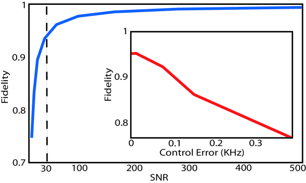
Figure 1: Quantum state reconstruction of the ”cat” state described in the text, for the $F=3$ hyperfine ground state of ${}^{133}\text{Cs}$ probed on the D1 transition. The figure shows the fidelity of reconstruction as a function of the measurement signal-to- noise ratio. Large nonlinearity and little decoherence allows good fidelity reconstruction in a single run, as indicated by the dashed line where a fidelity $\mathcal{F}=0.95$ is reached already at a very modest SNR of 30. The inset shows how the reconstruction degrades due to errors in the control field, at a constant SNR of 30. For a reasonable $1\%$ control field error the fidelity drops to $\mathcal{F}=0.85$.

The dynamical generation of a complete set of measurements incurs an unavoidable decoherence cost and so must be done as efficiently as possible. To this end we optimize based on a cost function consisting of the entropy $S(\mathcal{R})$ (Eq. 5) and any additional control costs $C(\mathbf{B})$. In this case the additional costs include the degradation in reconstruction due to loss of field control at large amplitudes, and inability to rapidly change the fields. We minimize these costs over all possible time dependent magnetic fields $\mathbf{B}(t)$. This is done sequentially, first restricting the magnetic fields to optimize the control costs $C(\mathbf{B})$, and then optimizing the entropy subject to these restrictions. The magnetic fields is restricted to be in the $x-y$ plane, with magnitude $|\mathbf{B}|=B$, such that the Larmor frequency is $\omega_{B}=\mu_{B}B/h=15$ kHz. Additionally we specify the field at only $n=50$ independent times and smoothly interpolate between them to ensure slow variation. The only free parameters are thus a set of $n=50$ indepedent angles. Optimizing the entropy subject to these constraints, we find that the landscape has many local minima, precluding the use of purely local search techniques. Instead, we use a one dimensional global search, where we iteratively optimize one of the $n=50$ independent angles, holding the others fixed. This process is repeated until all of the angles are globally stationary, within some tolerance, assuming the others are held fixed. This procedure is suboptimal, but converges reasonably well.

The results of simulated reconstructions are shown in Figs. 1 and 2. Given an initial preparation in the $F=3$ hyperfine manifold, in the “cat state” $\left|\psi_{0}\right\rangle=(\left|m=3\right\rangle+\left|m=-3\right\rangle)/\sqrt{2}$, the fidelity of the reconstruction, $\mathcal{F}=\left\langle\psi_{0}\right|\hat{\rho}_{\text{pos}}\left|\psi_{0}\right\rangle$, averaged over 1000 noise realizations, is plotted versus simulated SNR. Increasing SNR clearly results in a better reconstruction. The parameters needed to attain good fidelity for reconstruction of the $F=3$ ground state using the D1 transition (Fig. 1) appear to be well within the reach of current experiments at $\mathcal{F}\approx.95,\text{SNR}=30$ Smith03 . Even with a possible $1\%$ uncertainty in the control fields, a fidelity of $\mathcal{F}=.85$ should be possible (Fig. 1 inset). A different regime is illustrated by reconstruction of a spin $F=4$ using the D2 resonance. This turns out to be infeasible with a single measurement run performed on a single ensemble, even assuming very large SNR (Fig. 2). This is because more parameters must be reconstructed, $80$ versus $48$, and because the decoherence incurred in conjunction with the nonlinearity is larger due to the smaller hyperfine splitting of the $P_{3/2}$ manifold. It is still possible, however, to obtain a high fidelity reconstruction if we combine the measurement records from multiple independent runs that each start with a fresh ensemble and explore operator space in different ways.

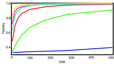
Figure 2: Quantum state reconstruction for the $F=4$ hyperfine state probed on the D2 transition, where the nonlinearity is weaker than for the case in Fig. 1. The curves correspond to an increasing number of independent runs, which allow increasingly complete exploration of the operator space. From lowest to highest fidelity we use: 1 run (blue), 2 runs (green), 3 runs (red), 4 runs (cyan), 5 runs (magenta), and 6 runs (yellow).

We have presented a new protocol for quantum state reconstruction based on continuous measurement of an ensemble of $N$ members and demonstrated our procedure through a simulated reconstruction of a spin $J$ via polarization spectroscopy of a gas of cold atoms. The reconstruction technique is nondestructive and exploits classical estimation theory, providing a starting point for consideration of more complex applications of quantum control tasks such as quantum feedback. In the future work we plan to improve our optimization procedure for robustness in control-parameter uncertainty and examine global search procedures such as convex optimization Vandenberghe96 . The tools developed here should provide new avenues for real-time state quantum estimation that allow us to explore the dynamical generation of nonclassical features, such as entanglement. This is of particular interest for mesoscopic systems whose classical description exhibits chaos Lakshminarayan01 .

- (1) M. A. Nielsen and I. L. Chuang, Quantum Computation and Quantum Information (Cambridge University Press, Cambridge, 2000)
- (2) JM Geremia et al., Phys. Rev. Lett. 91, 250801 (2003).
- (3) JM Geremia, J. K. Stockton and H. Mabuchi, Science 304, 270 (2004); JM Geremia, J. K. Stockton, and H. Mabuchi, quant- ph/0401107 (2004).
- (4) D. T. Smithey et al., Phys. Rev. Lett. 70, 1244 (1993).
- (5) T. J. Dunn, I. A. Walmsley, and S. Mukamel, Phys. Rev. Lett. 74, 884 (1995).
- (6) D. Leibfried et al., Phys. Rev. Lett. 77, 4281 (1996).
- (7) C. Kurtsiefer, T. Pfau, and J. Mlynek, Nature 386, 150 (1997).
- (8) I. L. Chuang, N. Gershenfeld, and M. Kubinec, Phys. Rev. Lett. 80, 3408 (1998)
- (9) G. Klose, G. Smith, P. S. Jessen, Phys. Rev. Lett. 86, 4721 (2001).
- (10) A. G. White et al., Phys. Rev. Lett. 83, 3103 (1999).
- (11) K. Mølmer, and L. B. Madsen, quant-ph/0402158 (2004).
- (12) G. A. Smith, S. Chaudhury, and P. S. Jessen, J. Opt. B 5, 323 (2003).
- (13) A. Kuzmich, L. Mandel, and N. P. Bigelow, Phys. Rev. Lett. 85, 1594 (2000).
- (14) C. M. Caves, J. Supercond. 12, 707 (1999).
- (15) L. Vandenberghe and S. Boyd, SIAM Review 38, 49 (1996).
- (16) G. A. Smith et al. Phys. Rev. Lett. 93, 163602 (2004).
- (17) C. Cohen-Tannoudji, J. Dupont-Roc and G. Grynberg, Atom-Photon Interactions, (Wiley, New York, 1992).
- (18) A. Lakshminarayan, Phys. Rev. E 64, 036207(2001).