Finite dimensional quantizations of the $(q,p)$ plane : new space and momentum inequalities.

Abstract:

We present a $N$-dimensional quantization à la Berezin-Klauder or frame quantization of the complex plane based on overcomplete families of states (coherent states) generated by the $N$ first harmonic oscillator eigenstates. The spectra of position and momentum operators are finite and eigenvalues are equal, up to a factor, to the zeros of Hermite polynomials. From numerical and theoretical studies of the large $N$ behavior of the product $\lambda_{m}(N)\,\lambda_{M}(N)$ of non null smallest positive and largest eigenvalues, we infer the inequality $\delta_{N}(Q)\,\Delta_{N}(Q)=\sigma_{N}\overset{<}{\underset{N\to\infty}{\to}}2\pi$ (resp. $\delta_{N}(P)\,\Delta_{N}(P)=\sigma_{N}\overset{<}{\underset{N\to\infty}{\to}}2\pi$) involving, in suitable units, the minimal ($\delta_{N}(Q)$) and maximal ($\Delta_{N}(Q)$) sizes of regions of space (resp. momentum) which are accessible to exploration within this finite-dimensional quantum framework. Interesting issues on the measurement process and connections with the finite Chern-Simons matrix model for the Quantum Hall effect are discussed.

1 Introduction

The idea of exploring various aspects of Quantum Mechanics by restricting the Hilbertian framework to finite-dimensional space has been increasingly used in the last decade, mainly in the context of Quantum Optics [1, 2], but also in the perpective of non-commutative geometry and “fuzzy” geometric objects [3]. For Quantum Optics, a comprehensive review (mainly devoted to the Wigner function) is provided by Ref.[4]. In [2], the authors defined normalized finite-dimensional coherent states by truncating the Fock expansion of the standard coherent states. Besides, basic features of the quantum Hall effect can be described within the finite matrix Chern-Simons approach [5].

It is well known, essentially since Klauder and Berezin, that one can easily achieve canonical quantization of the classical phase space by using standard coherent states [6, 7, 8, 9, 10]. In this paper we apply a related quantization method to the case in which the space of quantum states is finite-dimensional. Interesting new inequalities concerning observables emerge from this finite-dimensional quantization, in particular in the context of the quantum Hall effect.

This coherent state quantization with its various generalizations reveals itself as an efficient tool for quantizing physical systems for which the implementation of more traditional methods is unmanageable (see for instance [11, 12, 13]). In order to become familiar with our approach, we start the body of the paper by presenting in Section 2 the general mathematical framework, and we apply in Section 3 this formalism to the elementary example of the motion of the particle on the real line. We next consider in Section 4 finite-dimensional quantizations. After working out the algebras of these quantum systems, we shall explore their respective physical meaning in terms of lower symbols, localisation and momentum range properties. New inequalities are derived in Section 5. More precisely, from the existence of a finite spectrum of the position and momentum operators in finite-dimensional quantization, we find that there exists an interesting correlation between the size $\delta_{N}$ of the minimal “forbidden” cell and the width $\Delta_{N}$ of the spectrum (“size of the universe” accessible to measurements from the point of view of the specific system being quantized). This correlation reads in appropriate units $\delta_{N}\times\Delta_{N}=\sigma_{N}$, and numerical explorations, validated by theoretical arguments, indicate that the strictly increasing sequence converges: $\sigma_{N}\xrightarrow[N\to\infty]{}\sigma\sim 2\pi$. A similar result holds for the spectra of the momentum operators. In Section 6, we sketch a discussion about the consequences of our inequalities in term of physical interpretation, particularly in connection with the quantum Hall matrix model.

2 General setting: quantum processing of a measure space

In this section, we present the method of quantization we will apply in the sequel to a simple model, for instance the motion of a particle on the line, or more generally a system with one degree of freedom. The method, which is based on coherent states [9, 14] or frames [15] in Hilbert spaces is inspired by previous approaches proposed by Klauder [6, 10] and Berezin [7]. More details and examples concerning the method can be found in the references [11, 12, 13].

Let us start with an arbitrary measure space $(X,\mu)$. This set might be a classical phase space, but actually it can be any set of data accessible to observation. The existence of a measure provides us with a statistical reading of the set of measurable real- or complex-valued functions $f(x)$ on $X$: computing for instance average values on subsets with bounded measure. Actually, both approaches deal with quadratic mean values and correlation/convolution involving pairs of functions, and the natural framework of studies is the complex (Hilbert) spaces, $L^{2}(X,\mu)$ of square integrable functions $f(x)$ on $X$: $\int_{X}|f(x)|^{2}\,\mu(dx)<\infty$. One will speak of finite-energy signal in Signal Analysis and of (pure) quantum state in Quantum Mechanics. However, it is precisely at this stage that “quantum processing” of $X$ differs from signal processing on at least three points:

1. not all square integrable functions are eligible as quantum states,

2. a quantum state is defined up to a nonzero factor,

3. those ones among functions $f(x)$ that are eligible as quantum states with unit norm, $\int_{X}|f(x)|^{2}\,\mu(dx)=1$, give rise to a probability interpretation : $X\supset\Delta\rightarrow\int_{\Delta}|f(x)|^{2}\mu(dx)$ is a probability measure interpretable in terms of localisation in the measurable $\Delta$. This is inherent to the computing of mean values of quantum observables, (essentially) self-adjoint operators with domain included in the set of quantum states.

The first point lies at the heart of the quantization problem: what is the more or less canonical procedure allowing to select quantum states among simple signals? In other words, how to select the right (projective) Hilbert space ${\mathcal{H}}$, a closed subspace of $L^{2}(X,\mu)$, (resp. some isomorphic copy of it) or equivalently the corresponding orthogonal projecteur $I_{{\mathcal{H}}}$ (resp. the identity operator)?

In various circumstances, this question is answered through the selection, among elements of $L^{2}(X,\mu)$, of an orthonormal set $\mathcal{S}_{N}=\{\phi_{n}(x)\}_{n=0}^{N-1}$, $N$ being finite or infinite, which spans, by definition, the separable Hilbert subspace ${\mathcal{H}}\equiv{\mathcal{H}}_{N}$. The crucial point is that these elements have to fulfill the following condition :

$${\cal N}(x)\equiv\sum_{n}|\phi_{n}(x)|^{2}<\infty\ \mbox{almost everywhere}.$$ (1)

Of course, if $N\geq 1$ is finite the above condition is trivially checked.

We now consider the family of states $\{|x\rangle\}_{x\in X}$ in ${\mathcal{H}}_{N}$ obtained through the following linear superpositions:

$$|x\rangle\equiv\frac{1}{\sqrt{{\mathcal{N}}(x)}}\sum_{n}\overline{\phi_{n}}(x)|\phi_{n}\rangle,$$ (2)

in which the ket $|\phi_{n}\rangle$ designates the element $\phi_{n}(x)$ in a “Fock” notation and $\overline{\phi_{n}}(x)$ is the complex conjugate of $\phi_{n}(x)$. This defines an injective map

$$X\ni x\rightarrow|x\rangle\in{\mathcal{H}}_{N},$$ (3)

and the above Hilbertian superposition makes sense provided that set $X$ is equipped of a mild topological structure for which this map is continuous. It is not difficult to check that states (2) are coherent in the sense that they obey the following two conditions:

• Normalisation

  $$\langle\,x\,|x\rangle=1,$$ (4)

• Resolution of the unity in ${\mathcal{H}}_{N}$

  $$\int_{X}|x\rangle\langle x|\,\,\nu(dx)=I_{{\mathcal{H}}_{N}},$$ (5)

  where $\nu(dx)={\mathcal{N}}(x)\,\mu(dx)$ is another measure on $X$, absolutely continuous with respect to $\mu(dx)$. The coherent states (2) form in general an overcomplete (continuous) basis of ${\mathcal{H}}_{N}$. Actually, the term of frame [15] is more appropriate for designating the total family $\{|x\rangle\}_{x\in X}$.

The resolution of the unity in ${\mathcal{H}}_{N}$ can alternatively be understood in terms of the scalar product $\langle\,x\,|x^{\prime}\rangle$ of two states of the family. Indeed, (5) implies that, to any vector $|\phi\rangle$ in ${\mathcal{H}}_{N}$ one can isometrically associate the function

$$\phi(x)\equiv\sqrt{\mathcal{N}(x)}\langle x\,|\phi\rangle$$ (6)

in $L^{2}(X,\mu)$, and this function obeys

$$\phi(x)=\int_{X}\sqrt{\mathcal{N}(x)\mathcal{N}(x^{\prime})}\langle x|x^{\prime}\rangle\phi(x^{\prime})\,\mu(dx^{\prime}).$$ (7)

Hence, ${\mathcal{H}}_{N}$ is isometric to a reproducing Hilbert space with kernel

$${\cal K}(x,x^{\prime})=\sqrt{\mathcal{N}(x)\mathcal{N}(x^{\prime})}\langle x\,|x^{\prime}\rangle,$$ (8)

and the latter assumes finite diagonal values (a.e.), ${\cal K}(x,x)=\mathcal{N}(x)$, by construction.

A classical observable is a function $f(x)$ on $X$ having specific properties in relationship with some supplementary structure allocated to $X$, namely topology, geometry …. Its quantization simply consists in associating to $f(x)$ the operator

$$A_{f}:=\int_{X}f(x)|x\rangle\langle x|\,\nu(dx).$$ (9)

In this context, $f(x)$ is said upper (or contravariant) symbol of the operator $A_{f}$ and denoted by $f=\hat{A}_{f}$, whereas the mean value $\langle x|A|x\rangle$ is said lower (or covariant) symbol of an operator $A$ acting on ${\mathcal{H}}_{N}$ [7] and denoted by $\check{A}_{f}$. Through this approach, one can say that a quantization of the observation set is in one-to-one correspondence with the choice of a frame in the sense of (4) and (5). To a certain extent, a quantization scheme consists in adopting a certain point of view in dealing with $X$. This frame can be discrete, continuous, depending on the topology furthermore allocated to the set $X$, and it can be overcomplete, of course. The validity of a precise frame choice with regard to a certain physical context is asserted by comparing spectral characteristics of quantum observables $A_{f}$ with experimental data.

3 The standard case

Let us illustrate the above construction with the well-known Klauder-Glauber-Sudarshan coherent states [9]. The observation set $X$ is the classical phase space $\mathbb{R}^{2}\simeq\mathbb{C}=\{x\equiv z=\dfrac{1}{\sqrt{2m\omega u_{A}}}(m\omega q+ip)\}$ (in complex notations) of a system with one degree of freedom and experiencing a motion with characteristic time $\omega^{-1}$ and action $u_{A}$. Note that the characteristic length and momentum of this system are $l_{c}=\sqrt{\dfrac{u_{A}}{m\omega}}$ and $p_{c}=\sqrt{m\omega u_{A}}$ respectively, whereas the phase-space variable $z$ can be expressed in units of square root of action $\sqrt{u_{A}}$. Now, we could as well deal with an oscillating system like a biatomic molecule. Of course, in the domain of validity of quantum mechanics, it is natural to choose $u_{A}=\hbar$. The measure on $X$ is gaussian, $\mu(dx)=\frac{1}{\pi}\,e^{-\frac{|z|^{2}}{u_{A}}}\,d^{2}z$ where $d^{2}z$ is the Lebesgue measure of the plane. In the sequel, we shall work in suitable units, i.e. with $m=1$, $\omega=1$, and $u_{A}=1$.

The functions $\phi_{n}(x)$ are the normalised powers of the conjugate of the complex variable $z$, $\phi_{n}(x)\equiv\frac{\bar{z}^{n}}{\sqrt{n!}}$, so that the Hilbert subspace ${\cal H}$ is the so-called Fock-Bargmann space of all anti-entire functions that are square integrable with respect to the gaussian measure. Those states are eigenvectors of the number operator $\mathfrak{N}$ which is identical to the dilation operator $\mathfrak{N}=z\frac{\partial}{\partial z}$. Since $\sum_{n}\frac{|z|^{2n}}{n!}=e^{|z|^{2}}$, the coherent states read

$$|z\rangle=e^{-\frac{|z|^{2}}{2}}\sum_{n}\frac{z^{n}}{\sqrt{n!}}|n\rangle,$$ (10)

where we have adopted the usual notation $|n\rangle=|\phi_{n}\rangle$.

One easily checks the normalisation and unity resolution:

$$\langle z\,|z\rangle=1,\ \ \frac{1}{\pi}\int_{\mathbb{C}}|z\rangle\langle z|\,d^{2}z=I_{{\cal H}},$$ (11)

Note that the reproducing kernel is simply given by $e^{\bar{z}z^{\prime}}$. The quantization of the observation set is hence achieved by selecting in the original Hilbert space $L^{2}(\mathbb{C},\frac{1}{\pi}e^{-|z|^{2}}\,d^{2}z)$ all anti-holomorphic entire functions, which geometric quantization specialists would call a choice of polarization. Quantum operators acting on ${\cal H}$ are yielded by using (9). We thus have for the most basic one,

$$\frac{1}{\pi}\int_{\mathbb{C}}z\,|z\rangle\langle z|\,d^{2}z=\sum_{n}\sqrt{n+1}|n\rangle\langle n+1|\equiv a,$$ (12)

which is the lowering operator, $a|n\rangle=\sqrt{n}|n-1\rangle$. Its adjoint $a^{\dagger}$ is obtained by replacing $z$ by $\bar{z}$ in (12), and we get the factorisation $\mathfrak{N}=a^{\dagger}a$ together with the commutation rule $[a,a^{\dagger}]=I_{{\cal H}}$. Also note that $a^{\dagger}$ and $a$ realize on ${\cal H}$ as multiplication operator and derivation operator respectively, $a^{\dagger}f(z)=zf(z),\ af(z)=df(z)/dz$. From $q=\frac{1}{\sqrt{2}}(z+\bar{z})$ and $p=\frac{1}{i\sqrt{2}}(z-\bar{z})$, one easily infers by linearity that $q$ and $p$ are upper symbols for $\frac{1}{\sqrt{2}}(a+a^{\dagger})\equiv Q$ and $\frac{1}{i\sqrt{2}}(a-a^{\dagger})\equiv P$ respectively. In consequence, the self-adjoint operators $Q$ and $P$ obey the canonical commutation rule $[Q,P]=iI_{{\cal H}}$, and for this reason fully deserve the name of position and momentum operators of the usual (galilean) quantum mechanics, together with all localisation properties specific to the latter.

These standard states have many interesting properties. Let us recall two of them: they are eigenvectors of the lowering operator, $a|z\rangle=z|z\rangle$, and they saturate the Heisenberg inequalities : $\Delta Q\,\Delta P=\frac{1}{2}$. It should be noticed that they also pertain to the group theoretical construction since they are obtained from unitary Weyl-Heisenberg transport of the ground state: $|z\rangle=\exp(za^{\dagger}-\bar{z}a)|0\rangle$.

4 The finite-dimensional quantization

Let us now consider the generic orthonormal set with $N$ elements:

$$\phi_{0}(x)=1,\phi_{1}(x)=\bar{z},\dotsc\phi_{N-1}(x)=\frac{\bar{z}^{(N-1)}}{\sqrt{(N-1)!}}.$$ (13)

The coherent states read :

$$|z\rangle=\frac{1}{\sqrt{\mathcal{N}(x)}}\sum_{n=0}^{N-1}\frac{z^{n}}{\sqrt{n!}}|n\rangle,$$ (14)

with

$$\mathcal{N}(x)=\sum_{n=0}^{N-1}\frac{|z|^{2n}}{n!}.$$ (15)

They provide the following quantization of the classical position $q$ and momentum $p$ :

$$\frac{1}{\pi}\int_{\mathbb{C}}\left\{\begin{array}[]{c}q\\ p\end{array}\right\}|z\rangle\langle z|\mathcal{N}(x)e^{-|z|^{2}}\,d^{2}z=\left\{\begin{array}[]{c}Q_{N}\\ P_{N}\end{array}\right\}$$ (16)

Matrix elements of the position operator $Q_{N}$ and momentum operator $P_{N}$ are given by

$$Q_{N}(k,l)=\frac{1}{\sqrt{2}}\,(\sqrt{k}\,\delta_{k,l-1}\,+\sqrt{k-1}\,\delta_{k,l+1}\,),$$ (17)

$$P_{N}(k,l)=-i\,\frac{1}{\sqrt{2}}\,(\sqrt{k}\,\delta_{k,l-1}\,-\sqrt{k-1}\,\delta_{k,l+1}\,),$$ (18)

for $\ 1\leq k,l\leq N$. Their commutator is “almost” canonical:

$$[Q_{N},P_{N}]=iI_{N}-iNE_{N},$$ (19)

where $E_{N}$ is the orthogonal projector on the last basis element,

$$E_{N}=\left(\begin{array}[]{ccc}0&\dotso&0\\ \vdots&\ddots&\vdots\\ 0&\dotso&1\end{array}\right).$$

The appearing of such a projector in (19) is clearly a consequence of the truncation at the $N^{\mathrm{th}}$ level. We shall study the spectra of these operators in the next section.

The corresponding truncated harmonic oscillator hamiltonian $H_{N}=\dfrac{1}{2}(P_{N}^{2}+Q_{N}^{2})$ is diagonal with matrix elements :

$$H_{N}(k,l)=\frac{1}{2}\,(2k-1-N\delta_{k,N})\,\delta_{k,l}.$$ (20)

Since $H_{N}$ is diagonal, its eigenvalues are trivially $\frac{1}{2}\,(2k-1-N\delta_{N,k})$ and are identical to the lowest eigenenergies of the harmonic oscillator, except for the $N^{\mbox{th}}$ one which is equal to $\dfrac{N-1}{2}$ instead of $N-\dfrac{1}{2}$. One should notice that its nature differs according to the parity of $N$: it is degenerate if $N$ is even since then $\dfrac{N}{2}-\dfrac{1}{2}$ is already present in the spectrum whereas it assumes the intermediate value $\left\lfloor\dfrac{N}{2}\right\rfloor$ between two expected values if $N$ is odd.

Let us now consider the mean values or lower symbols of the position and momentum operators. We find:

$$\langle z|Q_{N}|z\rangle=C(|z|)q,\ \langle z|P_{N}|z\rangle=C(|z|)p,$$ (21)

where the corrective factor

$$C(|z|)=\frac{1}{\mathcal{N}(z)}\sum_{j=1}^{N-1}\frac{(|z|)^{2(j-1)}}{(j-1)!}$$ (22)

goes to $1$ as $N\to\infty$.

Lower symbols of the operators $Q_{N}^{2}$, $P_{N}^{2}$ and $H_{N}$ are given by:

$$\langle z|\left\{\begin{array}[]{l}Q_{N}^{2}\\ P_{N}^{2}\end{array}\right\}|z\rangle=A(|z|)\pm B(|z|),\ \langle z|H_{N}|z\rangle=A(|z|),$$ (23)

where

$$A(|z|) =\frac{1}{\mathcal{N}(z)}\sum_{k=1}^{N}\frac{|z|^{2(k-1)}}{(k-1)!}\,\left(\frac{2k-1-N\delta_{N,k}}{2}\right),$$

$$B(|z|) =\frac{1}{\mathcal{N}(z)}\sum_{k=1}^{N-2}\frac{|z|^{2(k-1)}}{(k-1)!}\,\frac{z^{2}+\bar{z}^{2}}{2}.$$

The behavior of these lower symbols in (23) in function of $(q,p)$, with the particular value $N=12$, is shown in Fig. 2. One can see that these mean values are identical, albeit the lower symbol of $P_{N}^{2}$ is obtained from that of $Q_{N}^{2}$ through a rotation by $\frac{\pi}{2}$ in the complex plane.

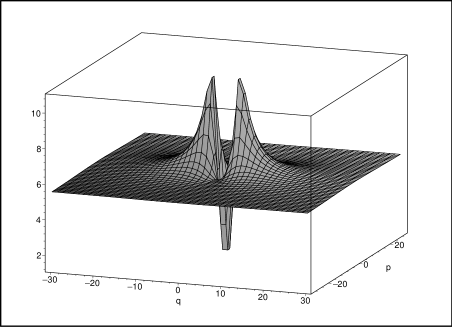
Figure 1: $(q,p)$ behavior of the meanvalues (lower symbols) of the operator $Q_{N}^{2}$ in the coherent state $|z\rangle$ for $N=12$.

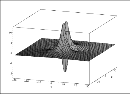
Figure 2: $(q,p)$ behavior of the meanvalues (lower symbols) of the operator $P_{N}^{2}$ in the coherent state $|z\rangle$ for $N=12$.

From all these meanvalues we can deduce the product $\Delta Q_{N}\,\Delta P_{N}$, where $\Delta Q_{N}=\sqrt{\langle z|Q_{N}^{2}|z\rangle-(\langle z|Q_{N}|z\rangle)^{2}}$. Due to rotational invariance, it is enough to consider its behavior in function of $q$, at $p=0$, as is shown in Fig. 3 for different values of $N$, $N=2,5,10,15$. One can observe that $\Delta Q_{N}\,\Delta P_{N}=1/2$, i.e. the product assumes, at the origin of the phase space the minimal value it would have in the infinite-dimensional case (with $\hbar=1$). Note that, for the minimal case $N=2$, the value $1/2$ is a supremum (!), and the latter is reached for almost all values of $z$ except in the range ${|z|\lesssim 10}$. For higher values of $N$, there exists around the origin a range of values of $|z|$, where the product is equal to $\frac{1}{2}$. This range increases with $N$ as expected since the Heisenberg inequalities are saturated with standard coherent states ($N=\infty$).

Figure 3: Behavior of $\Delta Q_{N}\,\Delta P_{N}$ in function of $q$, at $p=0$, for different values of $N$, $N=2$ (lowest curve), $5,10,15$ (upper curve).

Let us finally consider the behavior in function of $|z|$ of the lower symbol of the harmonic oscillator Hamiltonian given in Eq. (23). From Figs. 4 and 5 in which are shown respectively the meanvalue of $H_{N}$ at $N=5$, and the energy spectrum for different values of $N$, one can see the influence of truncating the dimension of the space of states.

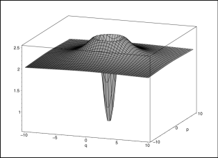
Figure 4: Meanvalue $\langle z|H_{N}|z\rangle$ of the harmonic oscillator hamiltonian as a function of $z=\frac{1}{\sqrt{2}}(q+ip)$ for $N=5$.

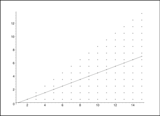
Figure 5: Spectrum of the harmonic oscillator Hamiltonian $H_{N}$ in function of $N$. One clearly sees the appearance of a degeneracy or an intermediate value instead in the vicinity of the middle of the spectrum, according to the parity of $N$, along the dotted line.

5 Localization and momentum of the finite-dimensional quantum system

We now examine the spectral features of the position and momentum operators $Q_{N}$, $P_{N}$ given in the $N$-dimensional case by Eqs.(24) and (25), i.e. in explicit matrix form by:

$$Q_{N}=\left(\begin{array}[c]{ccccc}0&\frac{1}{\sqrt{2}}&0&\dotso&0\\ \frac{1}{\sqrt{2}}&0&1&\dotso&0\\ 0&1&\ddots&\ddots&\vdots\\ \vdots&\dotso&\ddots&0&\sqrt{\frac{N-1}{2}}\\ 0&0&\dotso&\sqrt{\frac{N-1}{2}}&0\end{array}\right),$$ (24)

$$P_{N}=-i\left(\begin{array}[c]{ccccc}0&\frac{1}{\sqrt{2}}&0&\dotso&0\\ -\frac{1}{\sqrt{2}}&0&1&\dotso&0\\ 0&-1&\ddots&\ddots&\vdots\\ \vdots&\dotso&\ddots&0&\sqrt{\frac{N-1}{2}}\\ 0&0&\dotso&-\sqrt{\frac{N-1}{2}}&0\end{array}\right).$$ (25)

Their characteristic equations are the same. Indeed, $p_{N}(\lambda)=\det\left(Q_{N}-\lambda I_{N}\right)$ and $\det\left(P_{N}-\lambda I_{N}\right)$ both obey the same recurrence equation:

$$p_{N+1}(\lambda)=-\lambda p_{N}(\lambda)-\frac{N}{2}p_{N-1}(\lambda),$$ (26)

with $p_{0}(\lambda)=1$ and $p_{1}(\lambda)=-\lambda$. We have just to put $\mathrm{H}_{N}(\lambda)=(-2)^{N}p_{N}(\lambda)$ to ascertain that the $\mathrm{H}_{N}$’s are the Hermite polynomials for obeying the recurrence relation [16]:

$$\mathrm{H}_{N+1}(\lambda) =2\lambda\mathrm{H}_{N}(\lambda)-2N\mathrm{H}_{N-1}(\lambda),$$ (27)

$$\mathrm{H}_{0}(\lambda) =1,\ \mathrm{H}_{1}(\lambda)=2\lambda.$$

Hence the spectral values of the position operator, i.e. the allowed or experimentally measurable quantum positions, are just the zeros of the Hermite polynomials. The same result holds for the spectral values of the momentum operator.

The non-null roots of the Hermite polynomial $\mathrm{H}_{N}(\lambda)$ form the set

$$Z_{\mathrm{H}}(N) =\left\{-\lambda_{\left\lfloor\frac{N}{2}\right\rfloor}(N),-\lambda_{\left\lfloor\frac{N}{2}\right\rfloor-1}(N),\dotsc,-\lambda_{1}(N),\right.$$

$$\left.\lambda_{1}(N),\dotsc,\lambda_{\left\lfloor\frac{N}{2}\right\rfloor-1}(N),\lambda_{\left\lfloor\frac{N}{2}\right\rfloor}(N)\right\},$$ (28)

symmetrical with respect to the origin, where $\left\lfloor\frac{N}{2}\right\rfloor=\frac{N}{2}$ if $N$ is even and $\left\lfloor\frac{N}{2}\right\rfloor=\frac{N-1}{2}$ if N is odd; moreover $\mathrm{H}_{N}(0)=0$ if and only if $N$ is odd. A vast literature exists on the characterization and properties of the zeros of the Hermite polynomials, and many problems concerning their asymptotic behavior at large $N$ are still open. Recent results can be found in [17] with previous references therein. Upper bounds [18] have been provided for $\lambda_{m}(N)$ and $\lambda_{M}(N)$ where $\lambda_{m}(N)=\lambda_{1}(N)$ and $\lambda_{M}(N)=\lambda_{\left\lfloor\frac{N}{2}\right\rfloor}(N)$ are respectively the smallest and largest positive zeros of $\mathrm{H}_{N}$.

However, it seems that the following observation is not known. We have studied numerically the behavior of the product

$$\varpi_{N}=\lambda_{m}(N)\lambda_{M}(N)$$ (29)

The zeros of the Hermite polynomials have been computed by diagonalizing the matrix of the position operator $Q_{N}$; since $Q_{N}$ is tridiagonal symmetric with positive real coefficients, we implemented its diagonalization by using the QR algorithm [23]; such a method enabled us to compute the spectrum of the position operator up to the dimension $N=10^{6}$. The respective behaviors of $\lambda_{m}(N)$ and $\lambda_{M}(N)$ are shown in Fig. 6 for $N$ even and odd separately.

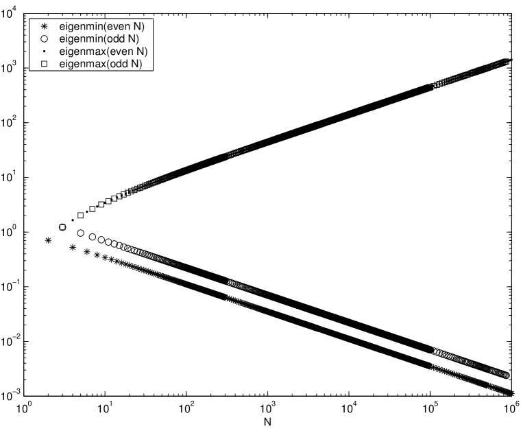
Figure 6: Bottom : behaviors of the lowest positive zero eigenmin($N$) $\equiv$ $\lambda_{m}(N)$ of the Hermite polynomial of degree $N$ for $N$ even and odd separately. Top : behavior of the largest positive zero eigenmax($N$) $\equiv$ $\lambda_{M}(N)$.

Now, one can easily check that $\lambda_{i+1}(N)-\lambda_{i}(N)>\lambda_{1}(N)$ for all $i\geq 1$ if $N$ is odd, whereas $\lambda_{i+1}(N)-\lambda_{i}(N)>2\lambda_{1}(N)$ for all $i\geq 1$ if $N$ is even, and that the zeros of the Hermite polynomials $\mathrm{H}_{N}$ and $\mathrm{H}_{N+1}$ intertwine, as is shown in Fig. 7 in the case of $\lambda_{m}(N)$ for small values of $N$.

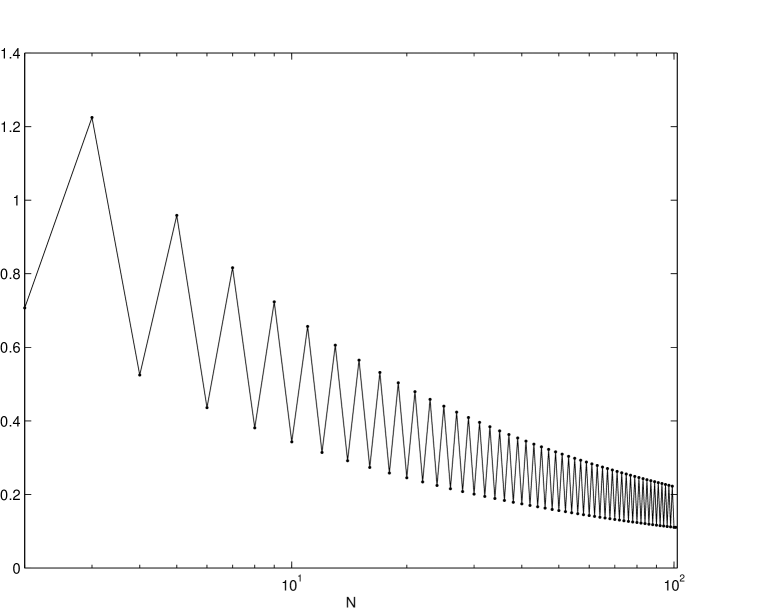
Figure 7: Intertwining of the lowest positive zeros $\lambda_{m}(N)$ of the Hermite polynomials $\mathrm{H}_{N}$ and $\mathrm{H}_{N+1}$ for small values of $N$.

On the other hand, the asymptotic behavior of $\lambda_{m}(N)$ and $\lambda_{M}(N)$ can be derived from the density distribution of the zeros of the Hermite polynomials for large $N$ [19]. This distribution obeys the Wigner semi-circle law [20, 21] that gives the asymptotic behavior of the number $n(x_{1},x_{2})$ of zeros lying in the interval $[x_{1},x_{2}]$

$$n(x_{1},x_{2})\underset{\mathrm{large}\,N}{\approx}N\int_{x_{1}}^{x_{2}}w(t)\,dt,$$ (30)

with

$$w(t)=\frac{1}{\pi N}\sqrt{2N-t^{2}}.$$ (31)

There follows from Eqs.(30,31) that the largest zero behaves like $\lambda_{M}(N)\underset{\mathrm{large}\,N}{\approx}\sqrt{2N}$, and the smallest positive zero behaves like $\lambda_{m}(N)\underset{\mathrm{large}\,N}{\approx}\pi/2\sqrt{2N}$ for even $N$, and like $\lambda_{m}(N)\underset{\mathrm{large}\,N}{\approx}\pi/\sqrt{2N}$ for odd $N$. Hence the asymptotical behaviors of the product $\varpi_{N}\stackrel{{\scriptstyle\mathrm{def}}}{{=}}\lambda_{m}(N)\lambda_{M}(N)$ read respectively:

$$\varpi_{N}=\lambda_{m}(N)\lambda_{M}(N)\underset{\mathrm{large}\,N}{\approx}\frac{\pi}{2},$$ (32)

for $N$ even, and

$$\varpi_{N}=\lambda_{m}(N)\lambda_{M}(N)\underset{\mathrm{large}\,N}{\approx}\pi$$ (33)

for $N$ odd.

Note that (32) and (33) could as well be derived from the asymptotic values of zeros of Laguerre polynomials [22].

Moreover, numerical studies show that the behavior of $\varpi_{N}$ is monotonically increasing for all even $N$ (resp. for all odd $N$). Therefore, if, at a given $N$, we define by $\Delta_{N}(Q)=2\lambda_{M}(N)$ the “size” of the “universe” accessible to exploration by the quantum system (or by the observer), and by $\delta_{N}(Q)=\lambda_{m}(N)$ (resp. $\delta_{N}(Q)=2\lambda_{m}(N)$) for odd (resp. even) $N$, the “size” of the smallest “cell” forbidden to exploration by the same system (or by the observer), we find the following upper bound for the product of these two quantities:

$$\delta_{N}(Q)\Delta_{N}(Q)\equiv\sigma_{N} =\left\{\begin{array}[c]{ll}4\lambda_{m}(N)\lambda_{M}(N)&\mbox{for}\ N\ \mbox{even},\\ 2\lambda_{m}(N)\lambda_{M}(N)&\mbox{for}\ N\ \mbox{odd},\end{array}\right.$$ (36)

$$\leq 2\pi.$$ (37)

The monotonically increasing behavior of the product $\sigma_{N}$, as a function of $N$, is shown in Fig. 8 and is also given in Table 1 where some values of $\sigma_{N}$ up to $N=10^{6}$ are given. .

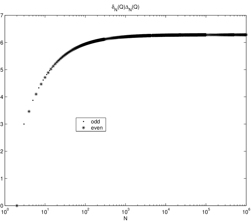
Figure 8: Behavior of the product $\sigma_{N}=\delta_{N}(Q)\Delta_{N}(Q)$, as a function of $N$.

Table 1: Values of $\sigma_{N}=\delta_{N}(Q)\Delta_{N}(Q)$ up to $N=10^{6}$. Compare with the value of $2\pi$.

Dimension $N$	$\delta_{N}(Q)\Delta_{N}(Q)$	$2\pi$
$10$	$4.713054$
$55$	$5.774856$
$100$	$5.941534$
$551$	$6.173778$
$1$ $000$	$6.209670$
$5$ $555$	$6.259760$
$10$ $000$	$6.267356$
$55$ $255$	$6.278122$
$100$ $000$	$6.279776$
$500$ $555$	$6.282020$
$1$ $000$ $000$	$6.282450$	6.2831853

Hence, we can assert the interesting inequality for the product (37):

$$\delta_{N}(Q)\Delta_{N}(Q)\leq 2\pi\ \forall N.$$ (38)

Identical result holds for the momentum, of course :

$$\delta_{N}(P)\Delta_{N}(P)\leq 2\pi\ \forall N.$$ (39)

6 Discussion

In order to fully perceive the physical meaning of such inequalities, it is necessary to reintegrate into them physical constants or scales proper to the considered physical system, i.e. characteristic length $l_{c}$ and momentum $p_{c}$ as was done at the beginning of Section 3:

$$\delta_{N}(Q)\Delta_{N}(Q) \leq 2\pi l^{2}_{c},$$ (40)

$$\delta_{N}(P)\Delta_{N}(P) \leq 2\pi p^{2}_{c}\ \forall N,$$ (41)

where $\delta_{N}(Q)$ and $\Delta_{N}(Q)$ are now expressed in unit $l_{c}$. Realistically, in any physical situation, $N$ cannot be infinite: there is an obvious limitation on frequencies or energies accessible to observation/experimentation. So it is natural to work with a finite although large value of $N$, which need not be determinate. In consequence, there exists irreducible limitations, namely $\delta_{N}(Q)$ and $\Delta_{N}(Q)$ in the exploration of small and large distances, and both limitations have the correlation (40).

Let us now suppose there exists, for theoretical reasons, a fundamental or “universal” minimal length, say $l_{m}$, something like the Planck length, or equivalently a universal ratio $\rho_{u}=l_{c}/l_{m}\geq 1$. Then, from $\delta_{N}(Q)\geq l_{m}$ and (38) we infer that there exists a universal maximal length $l_{M}$ given by

$$l_{M}\approx\sigma\rho_{u}l_{c}.$$ (42)

Of course, if we choose $l_{m}=l_{c}$, then the size of the “universe” is $l_{M}\approx 2\pi l_{m}$. Now, if we choose a characteristic length proper to Atomic Physics, like the Bohr radius, $l_{c}\approx 10^{-10}\mathrm{m}$, and for the minimal length the Planck length, $l_{m}\approx 10^{-35}\mathrm{m}$, we find for the maximal size the astronomical quantity $l_{M}\approx 10^{16}\mathrm{m}$. On the other hand, if we consider the (controversial) estimate size of our present universe $L_{u}=cT_{u}$, with $T_{u}\approx 13\,10^{9}$ years [24], we get from $l_{p}\,L_{u}\approx 2\pi l_{c}^{2}$ a characteristic length $l_{c}\approx 10^{-5}$m, i.e. a wavelength in the infrared electromagnetic spectrum…

Let us turn to another example, which might be viewed as more concrete, namely the quantum Hall effect in its matrix model version [5]. The planar coordinates $X_{1}$ and $X_{2}$ of quantum particles in the lowest Landau level of a constant magnetic field do not commute :

$$[X_{1},X_{2}]=i\theta.$$ (43)

where $\theta$ represents a minimal area. We recall that the average density of $N\to\infty$ electrons is related to $\theta$ by $\rho_{o}=1/2\pi\theta$ and the filling fraction is $\nu=2\pi\rho_{0}/B$. The quantity $l_{m}=\sqrt{\theta}$ can be considered as a minimal length. The Polychronakos model deals with finite number $N$ of electrons :

$$[X_{1,N},X_{2,N}]=i\theta(1-N|N-1\rangle\langle N-1|).$$ (44)

In this context, our inequalities read as

$$\delta_{N}(X_{i})\Delta_{N}(X_{i})\leq 2\pi l^{2}_{c},\ i=1,2,$$ (45)

where $l_{c}$ corresponds to a choice of experimental unit. Since $l_{m}=\sqrt{\theta}$ affords an irreducible lower limit in this problem, we can assert that the maximal linear size $L_{M}$ of the sample should satisfy :

$$l_{M}\leq 2\pi\frac{l_{c}}{\sqrt{\theta}}l_{c},$$ (46)

for any finite $N$.

The experimental interpretation of such a result certainly deserves a deeper investigation.

As a final comment concerning the inequalities (40) and (41), we would like to insist on the fact they are not just an outcome of finite approximations $Q_{N}$ and $P_{N}$ (or $X_{1,N}$ and $X_{2,N}$) to the canonical position and momentum operators (or to $X_{1}$ and $X_{2}$) in infinite-dimensional Hilbert space of quantum states. They hold however large the dimension $N$ is, as long as it is finite. Furthermore, let us advocate the idea that a quantization of the classical phase space results from the choice of a specific (reproducing) Hilbert subspace $\mathcal{H}$ in $L^{2}(\mathbb{R}^{2},d\mu(q,p))$ in which coherent states provide a frame resolving the identity. This frame corresponds to a certain point of view in dealing with the classical phase space, and this point of view yields the quantum versions $Q_{N}$ and $P_{N}$ (or $X_{1,N}$ and $X_{2,N}$) of the classical coordinates $q$ and $p$ (or $x_{1}$ and $x_{2}$).

- [1] V. Bužek, A. D. Wilson-Gordon, P. L. Knight, and W. K. Lai, Coherent states in a finite-dimensional basis : Their phase properties and relationship to coherent states of light, Phys. Rev. A 45 (1992) 8079
- [2] L. M. Kuang, F. B. Wang, and Y. G. Zhou, Dynamics of a harmonic oscillator in a finite-dimensional Hilbert space, Phys. Lett. A 183 (1993) 1; Coherent States of a Harmonic Oscillator in a Finite-dimensional Hilbert Space and Their Squeezing Properties, J. Mod. Opt. 41 (1994) 1307
- [3] A. A. Kehagias and G. Zoupanos, Finiteness due to cellular structure of , I. Quantum Mechanics, Z. Physik C 62 (1994) 121
- [4] A. Miranowicz, W. Leonski, and N. Imoto, Quantum-Optical States in Finite-Dimensional Hilbert Spaces. 1. General Formalism, in Modern Nonlinear Optics, ed. M. W. Evans, Adv. Chem. Phys. 119(I) (2001) 155 (Wiley, New York); [quant-ph/0108080]; ibidem 195; [quant-ph/0110146]
- [5] A. P. Polychronakos Quantum Hall states as matrix Chern-Simons theory, J. High Energy Phys. 04 (2001) 011
- [6] J. R. Klauder, Continuous-Representation Theory I. Postulates of continuous-representation theory, J. Math. Phys. 4 (1963) 1055; Continuous-Representation Theory II. Generalized relation between quantum and classical dynamics, J. Math. Phys. 4 (1963) 1058
- [7] F. A. Berezin, General concept of quantization, Commun. Math. Phys. 40 (1975) 153
- [8] J. R. Klauder and B.-S. Skagerstam (eds.), Coherent states. Applications in physics and mathematical physics, World Scientific Publishing Co., Singapore, 1985
- [9] D. H. Feng, J. R. Klauder, and M. Strayer, M. (eds.), Coherent States: Past, Present and Future (Proc. Oak Ridge 1993), World Scientific, Singapore, 1994
- [10] J. R. Klauder, Quantization without Quantization, Ann. Phys. (NY) 237 (1995) 147
- [11] T. Garidi, J-P. Gazeau, E. Huguet, M. Lachièze Rey, and J. Renaud, Examples of Berezin-Toeplitz Quantization: Finite sets and Unit Interval in Symmetry in Physics. In memory of Robert T. Sharp 2002 eds. P. Winternitz et al (Montréal: CRM Proceedings and Lecture Notes) 2004; Quantization of the sphere with coherent states in Classical, Stochastic and Quantum gravity, String and Brane Cosmology, Peyresq 2002, Int. J. Theor. Phys. 42 (2003) 1301, [http://arXiv.org/abs/math-ph/0302056]
- [12] S. T. Ali, M. Englis, and J-P. Gazeau, Vector Coherent States from Plancherel’s Theorem, Clifford Algebras and Matrix Domains, J. Phys. A 37 (2004) 6067
- [13] J-P. Gazeau and W. Piechocki, Coherent states quantization of a particle in de Sitter space, J. Phys. A 37 (2004) 6977
- [14] S. T. Ali, J-P. Antoine, and J-P. Gazeau, Coherent states, wavelets and their generalizations, Graduate Texts in Contemporary Physics, Springer-Verlag, New York, 2000
- [15] S. T. Ali, J-P. Antoine, and J-P. Gazeau, Continuous Frames in Hilbert Spaces Ann. Phys. (NY) 222 (1993) 1
- [16] Magnus, W., Oberhettinger, F., and Soni, R. P. : Formulas and Theorems for the Special Functions of Mathematical Physics, 3rd ed., Springer-Verlag, Berlin, Heidelberg and New York, 1966
- [17] A. Elbert, Some recent results on the zeros of Bessel functions and orthogonal polynomials, J. Comput. Appl. Math. 133 (2001) 65
- [18] I. Area, D. K. Dimitrov, E. Godoy, and A. Ronveaux, Zeros of Gegenbauer and Hermite polynomials and connection coefficients, Math. Comp. 73 (2004) 1937
- [19] D. S. Lubinsky, A Survey of General Orthogonal Polynomials for Weights on Finite and Infinite Intervals, Acta Applicandae Mathematicae 10 (1987) 237; An Update on Orthogonal Polynomials and Weighted Approximation on the Real Line, Acta Applicandae Mathematicae 33 (1993) 121
- [20] E. P. Wigner, Distribution of neutron resonance level spacing, Columbia University Report CU 175, 1957. [Reprinted in The Collected Works of Eugene Paul Wigner, Part A, Vol. II, Springer-Verlag, Berlin, 1996, 337]
- [21] A very pedagogical explanation of the semi-circle law is given in the Junior Research Seminar on Probability, -Functions, Random Matrix Theory and Ramanujan Graphs, online at http://www.math.princeton.edu/ mathlab/
- [22] M. Abramowitz, and I. A. Stegun, Handbook of Mathematical Functions, Tenth printing, National Bureau of Standards Applied Mathematics Series no. 55, Washington, 1972
- [23] W. H. Press, B. P. Flannery, S. A. Teukolsky, and W. T. Vetterling, Numerical Recipes, the Art of Scientific Computing, Cambridge University Press, 1986
- [24] L. Pasquini, P. Bonifacio, S. Randich, D. Galli, and R. G. Gratton, Beryllium in turnoff stars of NGC6397: early Galaxy spallation, cosmochronology and cluster formation, comments, to appear in A& A (2004)