Robust Quantum Algorithms for Oracle Identification

Abstract

The oracle identification problem (OIP) was introduced by Ambainis et al. [4]. It is given as a set $S$ of $M$ oracles and a blackbox oracle $f$. Our task is to figure out which oracle in $S$ is equal to the blackbox $f$ by making queries to $f$. OIP includes several problems such as the Grover Search as special cases. In this paper, we improve the algorithms in [4] by providing a mostly optimal upper bound of query complexity for this problem: ($i$) For any oracle set $S$ such that $|S|\leq 2^{N^{d}}$ ($d<1$), we design an algorithm whose query complexity is $O(\sqrt{N\log{M}/\log{N}})$, matching the lower bound proved in [4]. ($ii$) Our algorithm also works for the range between $2^{N^{d}}$ and $2^{N/\log{N}}$ (where the bound becomes $O(N)$), but the gap between the upper and lower bounds worsens gradually. ($iii$) Our algorithm is robust, namely, it exhibits the same performance (up to a constant factor) against the noisy oracles as also shown in the literatures [2, 12, 21] for special cases of OIP.

keywords: quantum computing, query complexity and algorithmic learning theory

1 Introduction

We study the following problem, called the Oracle Identification Problem (OIP): Given a hidden $N$-bit vector $f=(a_{1},\ldots,a_{N})\in\{0,1\}^{N}$, called an oracle, and a candidate set $S\subseteq\{0,1\}^{N}$, OIP requires us to find which oracle in $S$ is equal to $f$. OIP has been especially popular since the emergence of quantum computation, e.g., [7, 8, 9, 12, 14, 21]. For example, suppose that we set $S=\{(a_{1},\ldots,a_{N})|\mbox{~{}exactly one~{}}a_{i}=1\}$. Then this OIP is essentially the same as Grover search [20]. In [4], Ambainis et al. extended the problem to a general $S$. They proved that the total cost of any OIP with $|S|=N$ is $O(\sqrt{N})$, which is optimal within a constant factor since this includes the Grover search as a special case and for the latter an $\Omega(\sqrt{N})$ lower bound is known (e.g., [9]). For a larger $S$, they obtain nontrivial upper and lower bounds, $O(\sqrt{N\log{M}\log{N}}\log{\log{M}})$ and $\Omega(\sqrt{N\log{M}/\log{N}})$, respectively, but unfortunately, there is a fairly large gap between them.

Our Result.  Let $M=|S|$. ($i$) If $M\leq 2^{N^{d}}$ for a constant $d$ ($<1$), then the cost of our new algorithm is $O(\sqrt{N\log{M}/\log{N}})$ which matches the lower bound obtained in [4]. (Previously we have an optimal upper bound only for $M=N$). ($ii$) For the range between $2^{N^{d}}$ and $2^{N/\log{N}}$, our algorithm works without any modification and the (gradually growing) gap to the lower bound is at most a factor of $O(\sqrt{\log{N}\log\log{N}})$. ($iii$) Our algorithm is robust, namely, it exhibits the same performance (up to a constant factor) against the noisy oracles as shown in the literatures [2, 12, 21] for special cases of OIP.

Our algorithms use two operations: ($i$) The first one is a simple query (S-query) to the hidden oracle, i.e., to obtain the value ($0$ or $1$) of $a_{i}$ by specifying the $\log{N}$-bit index $i$. The cost for this query is one per each. ($ii$) The second one is called a G-query to the oracle: By specifying a set $T=\{i_{1},\ldots,i_{r}\}$ of indices, we can obtain, if any, an index $i_{j}\in T$ s.t. $a_{i_{j}}=1$ and nill otherwise. If there are two or more such $i_{j}$’s then one of them is chosen at random. The cost for this query is $O(\sqrt{|T|/K})$ where $K=\left|\{i_{j}|~{}i_{j}\in T\mbox{~{}and~{}}a_{i_{j}}=1\}\right|+1$. This query is stochastic, i.e., the answer is correct with a constant probability. Obviously our goal is to minimize the cost for solving the OIP with a constant success probability. Note that we incur the cost for only S- and G-queries (i.e., the cost for any other computation is zero), and it turns out that our query model is equivalent to the standard query complexity one, e.g., [6].

S-queries are standard and may not need any explanation. G-queries are, as one can see, the Grover Search themselves. So, they cannot be implemented in the framework of classical computation, and hence our paper is definitely a quantum paper. However, if we use the two queries as blackbox subroutines and follow the above complexity measure, then our algorithm design will be completely classical. Now it is important to observe the ”efficiency” of G-queries. Since its cost is sublinear in $|T|$, our general idea is that it is more cost-effective to use them for a larger $T$. For example, the cost for a single G-query for $|T|=L$ is less than the total cost of three G-queries for $|T^{\prime}|=L/3$. However, it is also true that the former is less informative since it gives us only one bit-position in $T$ which has value one, while the latter gives us three. Thus, as one would expect, selecting the size of $T$ is a key issue when using G-queries.

As mentioned earlier, if we use the two queries as blackbox subroutines together with their cost rule, then any knowledge about quantum computation is not needed in the design and analysis of our algorithms. Since $S$ is a set of $M$  $0/1$-vectors of length $N$, it is naturally given as a $0/1$ matrix $Z$ of $N$ columns and $M$ rows. For a given $Z$, our basic strategy is quite simple: if there is a column which includes a balanced number of $0$’s and $1$’s, then we ask the value of the oracle at that position by using an S-query. This reduces the number of candidates by a constant factor. Otherwise, i.e., if every column has, say, a small fraction of $1$’s, then S-queries may seldom reduce the candidates. In such a situation, the idea is that it is better to use a G-query by selecting a certain number of columns in $T$ than repeating S-queries. In order to optimize this strategy, our new algorithm controls the size of $T$ very carefully. This contrasts with the previous method [4] that uses G-queries always with $T=\{1,\ldots,N\}$

Previous Work. Suppose that we wish to solve some problem over input data of $N$ bits. Presumably, we need all the values of these $N$ bits to obtain a correct answer, which in turn requires $N$ (simple) queries to the data. In a certain situation, we do not need all the values, which allows us to design a variety of sublinear-time (classical) algorithms, e.g., [13, 19, 23]. This is also true when the input is given with some premise, for which giving a candidate set as in this paper is the most general method. Quickly approaching to the hidden data using the premise information is the basis of algorithmic learning theory. In fact, Atici et al. in [5] independently use techniques similar to ours in the context of quantum learning theory. One of their results, which states the existence of a quantum algorithm for learning a concept class $S$ whose parameter is $\gamma_{S}$ with $O(\log{|S|}\log{\log{|S|}}/\sqrt{\gamma_{S}})$ queries, almost establishes a conjecture of $O(\log{|S|}/\sqrt{\gamma_{S}})$ queries in [22].

Recall that our complexity measure is the (quantum) query complexity, which has been intensively studied as a central issue of quantum computation. The most remarkable result is due to Grover [20], which provided a number of applications and extensions, e.g., [8, 9, 14]. Recently quite many results on efficient quantum algorithms are shown by ”sophisticated” ways of using the Grover Search. (Our present paper is also in this category.) Brassard et al. [10] showed a quantum counting algorithm that gives an approximate counting method by combining the Grover Search with the quantum Fourier transformation. Quantum algorithms for the claw-finding and the element distinctness problems given by Buhrman et al. [11] also exploited classical random and sorting methods with the Grover Search. (Ambainis [3] developed an optimal quantum algorithm with $O(N^{2/3})$ queries for element distinctness problem, which makes use of the quantum walk and matches to the lower bounds shown by Shi [25].) Aaronson et al. [1] constructed quantum search algorithms for spatial regions by combining the Grover Search with the divided-and-conquer method. Magniez et al. [24] showed efficient quantum algorithms to find a triangle in a given graph by using combinatorial techniques with the Grover Search. Dürr et al. [16] also investigated quantum query complexity of several graph-theoretic problems. In particular, they exploited the Grover Search on some data structures of graphs for their upper bounds.

Recently, two papers, by Høyer et al. [21] and Buhrman et al. [12], raised the question of how to cope with “imperfect” oracles for the quantum case using the following model: The oracle returns, for the query to bit $a_{i}$, a quantum pure state from which we can measure the correct value of $a_{i}$ with a constant probability. This noise model naturally fits the motivation that a similar mechanism should apply when we use bounded-error quantum subroutines. In [21] Høyer et al. gave a quantum algorithm that robustly computes the Grover’s problem with $O(\sqrt{N})$ queries, which is only a constant factor worse than the noiseless case. Buhrman et al. [12] also gave a robust quantum algorithm to output all the $N$ bits by using $O(N)$ queries. This obviously implies that $O(N)$ queries are enough to compute the parity of the $N$ bits, which contrasts with the classical $\Omega(N\log N)$ lower bound given in [18]. Thus, robust quantum computation does not need a serious overhead at least for several important problems, including the OIP discussed in this paper.

2 S-queries, G-queries and Robustness

Recall that an instance of OIP is given as a set $S=\{f_{1},\ldots,f_{M}\}$ of oracles, each $f_{i}=(f_{i}(1),\ldots,f_{i}(N))\in\{0,1\}^{N}$, and a hidden oracle $f\in S$ which is not known in advance. We are asked to find the index $i$ such that $f=f_{i}$. We can access the hidden oracle $f$ through a unitary transformation $U_{f}$, which is referred to as an oracle call, such that

$$U_{f}\left|x\right>\left|0\right>=\left|x\right>\left|f(x)\right>,$$

where $1\leq x\leq N$ denotes the bit-position of $f$ whose value ($0$ or $1$) we wish to know. This bit-position might be a superposition of two or more bit-positions, i.e., $\sum_{i}\alpha_{i}\left|x_{i}\right>$. Then the result of the oracle call is also a superposition, i.e., $\sum_{i}\alpha_{i}\left|x_{i}\right>\left|f(x_{i})\right>$. The query complexity counts the number of oracle calls being necessary to obtain a correct answer $i$ with a constant probability.

In this paper we will not use oracle calls directly but through two subroutines, S-queries and G-queries. (Both can be viewed as classical subroutines when used.) An S-query, $\mbox{SQ}(i)$, is simply a single oracle call with the index $i$ plus observation. It returns $f(i)$ with probability one and its query complexity is obviously one. A G-query, $\mbox{GQ}(T)$, where $T\subseteq\{1,\ldots,N\}$, returns $1\leq i\leq N$ such that $i\in T$ and $f(i)=1$ if such $i$ exists and nill otherwise. We admit an error, namely, the answer may be incorrect but should be correct with a constant probability, say, $2/3$. Although details are omitted, it is easy to see that $\mbox{GQ}(T)$ can be implemented by applying Grover Search only to the selected positions $T$. Its query complexity is given by the following lemma.

Lemma 1 ([10])

$\mbox{GQ}(T)$ needs $O(\sqrt{|T|/K})$ oracle calls, where $K=\left|\{j|~{}j\in T\mbox{~{}and~{}}f(j)=1\}\right|+1$.

If $f$ is a noisy oracle, then its unitary transformation is given as follows [2]:

$$\tilde{U}_{f}\left|x\right>\left|0\right>\left|0\right>=\sqrt{p_{x}}\left|x\right>\left|\phi_{x}\right>\left|f(x)\right>+\sqrt{1-p_{x}}\left|x\right>\left|\psi_{x}\right>\left|\neg{f(x)}\right>,$$

where $2/3\leq p_{x}\leq 1$, $\left|\phi_{x}\right>$ and $\left|\psi_{x}\right>$ (the states of working registers) may depend on $x$. As before $\left|x\right>$ (and hence the result also) may be a superposition of bit-positions. Since an oracle call itself includes an error, an S-query should also be stochastic. $\tilde{\mbox{SQ}}(i)$ returns $f(i)$ with probability at least $2/3$ (and $\neg{f(i)}$ with at most $1/3$). G-queries, $\tilde{\mbox{GQ}}(T)$, are already stochastic, i.e., succeed to find an answer with probability at least $2/3$ if there exists one, and they do not need modification.

Lemma 2 ([21])

Let $K$ and $T$ be as before. Then $\tilde{\mbox{GQ}}(T)$ needs $O(\sqrt{|T|/K})$ noisy oracle calls.

In this paper our oracle mode is almost always noisy. Therefore we simply use the notation SQ and GQ instead of $\tilde{\mbox{SQ}}$ and $\tilde{\mbox{GQ}}$.

3 Algorithms for Small Candidate Sets

3.1 Overview of the Algorithm

Recall that the candidate set $S$ ($|S|=M)$ is given as an $M\times N$ matrix $Z$. Before we give our main result in the next section, we discuss the case that $Z$ is small, i.e., $M=\mbox{poly}(N)$ in this section, which we need in the main algorithm and also will be nice to understand the basic idea. Since our goal is to find a single row from the $M$ ones, a natural strategy is to reduce the number of candidate rows (a subset of rows denoted by $S$) step by step. This can be done easily if there is a column, say, $j$ which is “balanced,” i.e., which has an approximately equal number of $0$’s and $1$’s in $Z(S)$, where $Z(S)$ denotes the matrix obtained from $Z$ by deleting all rows not in $S$. Then by asking the value of $f(j)$ by an $\mbox{SQ}(j)$, we can reduce the size of $S$ (i.e., the number of oracle candidates) by a constant factor. Suppose otherwise, that there are no such good columns in $Z(S)$. Then we gather a certain number of columns such that the set $T$ of these columns is “balanced,” namely, such that the number of rows which has $1$ somewhere in $T$ is a constant fraction of $|S|$. (See Fig. 1 where the columns in $T$ are shifted to the left.) Now we execute $\mbox{GQ}(T)$ and we can reduce the size of $S$ by a constant fraction according to whether $\mbox{GQ}(T)$ returns nill ($S$ is reduced to $S_{2}$ in Fig. 1) or not ($S$ is reduced to $S_{1}$ in Fig. 1). Then we move to the next iteration until $|S|$ becomes one.

The merit of using $\mbox{GQ}(T)$ is obvious since it needs at most $O(\sqrt{|T|})$ queries while we may need roughly $|T|$ queries if asking each position by S-queries. Even so, if $|T|$ is too large, we cannot tolerate the cost for $\mbox{GQ}(T)$. So, the key issue here is to set a carefully chosen upper bound for the size of $T$. If we can select $T$ within this upper bound, then we are happy. Otherwise, we just give up constructing $T$ and use another strategy which takes advantage of the sparseness of the current matrix $Z(S)$. (Obviously $Z(S)$ is sparse since we could not select a $T$ of small size.)

It should be also noted that in each iteration the matrix $Z(S)$ should be one-sensitive, namely the number of 1’s is less than or equal to the number of 0’s in every column. (The reason is obvious since it does not make sense to try to find 1 if almost all entries are 1.) For this purpose we implicitly apply the column-flipping procedure in each iteration. Suppose that some column, say $j$, of $Z(S)$ has more 1’s than 0’s. Then this procedure “flips” the value of $f(j)$ by adding an extra circuit to the oracle (but without any oracle call). Let this oracle be $\overline{f(j)}$ and $\overline{Z(S(j))}$ be the matrix obtained by flipping the column $j$ of $Z(S)$. Then obviously $f\in S$ iff the matrix $\overline{Z(S(j))}$ contains the row $\overline{f(j)}$, i.e., the problem does not change essentially. Note that the column-flipping is the same as that in [4], where the OIP matrix was written as a $N\times M$ (number of columns $\times$ number of rows) $0$-$1$ matrix instead of the more common $M\times N$ one.

Figure 1: Reducing the candidate set by G-queries $\mbox{GQ}(T)$ on the column set $T$

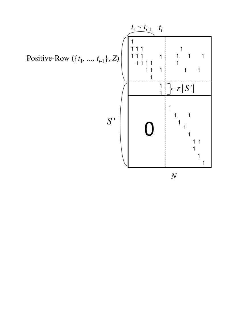
Figure 2: Constructing the column set $T$ by RowCover($S,r$)

3.2 Procedure RowReduction($T,l$) for Reducing Oracles Candidates

This procedure narrows $S$ in each iteration, where $T$ is a set of columns and $l$ is an integer $\geq 1$ necessary for error control. See Procedure 1 for its pseudocode. Case $1$: If $f$ has one or more $1$’s in $T$ like $f_{1}$ in Fig. 1, then $k=\mbox{GQ}(T)$ gives us one of the positions of these $1$’s, say the circled one in the figure. The procedure returns with the set $S_{1}^{\prime}$ of rows in the figure, i.e., the rows having a $1$ in the position selected by the $\mbox{GQ}(T)$. Case $2$: If $f$ has no $1$’s in $T$ like $f_{2}$ in the figure, then $k=\mbox{~{}nill}$ (i.e., $\mbox{GQ}(T)$ correctly answered). Even if $k\neq\mbox{~{}nill}$ ($\mbox{GQ}(T)$ failed) then $\mbox{Majority}(k,l,f)$, i.e., the majority of $60l$ samples of $f(k)$, is $0$ with high probability regardless of the value of $k$. Therefore the procedure returns with the set $S_{2}$ of rows, i.e., the rows having no $1$’s in $T$. The parameter $l$ guarantees the success probability of this procedure as follows.

Lemma 3

The success probability and the number of oracle calls in $\mbox{RowReduction}(T,l)$ are $1-O(l/3^{l})$ and $l(O(\sqrt{|T|})+l)$, respectively.

• In each repetition, we need $O(\sqrt{|T|})$ oracle calls for the G-queries and $O(l)$ calls (S-queries) for $\mbox{Majority}(k,l,f)$. Thus the total number of calls is $l(O(\sqrt{|T|})+l)$. For the success probability, let us first consider Case $1$ above. Since the G-queries are repeated up to $l$ times, the probability that all tries fail (i.e., the next $\mbox{Majority}=0$) is $1/3^{l}$. When it succeeds, the following Majority fails with probability $1/3^{l}$ also (Here, the number of samples ($=60l$) for majority is set appropriately so that the error probability is at most $1/3^{l}$ by the Chernoff bound). Hence the total failure probability is at most $O(1/3^{l})$. In Case $2$, since Majority fails with probability $O(1/3^{l})$ in each iteration, the total probability of failure is at most $O(l/3^{l})$.      

3.3 Procedure RowCover($S,r$) for Collecting Position of Queries

As mentioned in Sec. 3.1, we need to make a set $T$ of columns being balanced as a whole. This procedure is used for this purpose where $Z(S)$ is the current matrix and $0<r\leq 1$ controls the size of $T$. See Procedure 2 for its pseudocode. As shown in Fig. 2, the procedure adds columns $t_{1},t_{2},\ldots,$ to $T$ as long as a new addition $t_{i}$ increases the number of covered rows ($=|\mbox{PositiveRow}(T,Z)|$) by a factor of $r$ or until the number of covered rows becomes $|S|/4$. We say that RowCover succeeds if it finishes with $S^{\prime}$ such that $|S^{\prime}|\leq\frac{3|S|}{4}$ and fails otherwise. Suppose that we choose a smaller $r$. Then this guarantees that the resulting $Z(S)$ when RowCover fails is more sparse, which is desirable for us as described later. However since $|T|\leq 1/r$, a smaller $r$ means a larger $T$ when the procedure succeeds, which costs more for G-queries in RowReduction. Thus, we should choose the minimum $r$ such that the query complexity for the case that RowCover keeps succeeding as long as the total cost does not exceed the total limit ($=O(\sqrt{N})$).

3.4 Analysis of the Whole Algorithm

Now we are ready to prove our first theorem:

Theorem 1

The $M\times N$ OIP can be solved with a constant success probability by querying the blackbox oracle $O(\sqrt{N})$ times if $M=\mbox{poly}(N)$.

• See Procedure 5 for the pseudocode of the algorithm ROIPS($S,Z$) (Robust OIP algorithm for Small $Z$). We call this procedure with $S=\{1,\ldots,M\}$ (we need this parameter since ROIPS is also used in the later algorithm) and the given matrix $Z$. As described in Sec. 3.1, we narrow the candidate set $S$ at lines 2 and 3. If RowCover at line 2 succeeds, then $|S|$ is sufficiently reduced. Even if RowCover fails, $|S|$ is also reduced similarly if RowReduction at line 3 can find a $1$ by G-queries. Otherwise line 7 is executed where the current oracle looks like $f_{2}$ in Fig. 1. In this case, by finding a $1$ in the positions $\{1,\ldots,N\}\setminus{T}$ by the G-query at line 7, $|S|$ is reduced to $|S|\log^{4}{N}/N$, because we set $r=\log^{4}{N}/N$ at line 2. Since the original size of $S$ is $N^{c}$ for a constant $c$, line 7 is executed at most $c+1$ times.

  Note that the selection of the value of $r$ at line $2$ follows the rule described in Sec. 3.3: Since $r=\log^{4}{N}/N$, the size of $T$ at line 3 is at most $N/\log^{4}{N}$. This implies that the number of oracle calls at line 3 is $O(\log{N}\cdot\sqrt{N}/\log^{2}{N})=O(\sqrt{N}/\log{N})$. Since line 3 is repeated at most $O(\log{N})$ times, the total number of oracle calls at line 3 is at most $O(\sqrt{N})$. Line 7 needs $O(\sqrt{N})$ oracle calls, but the number of its repetitions is $O(1)$ as mentioned above. Thus the total number of oracle calls is $O(\sqrt{N})$.

  Also by Lemma 1, the error probability of line 3 is at most $O(\log{N}/N)$. Since the number of repetitions is $O(\log{N})$, this error probability is obviously small enough. The error probability of line 7 is constant but again this is not harmful since it is repeated only $O(1)$ times, and thus the error probability can be made as small as it is needed at constant cost.      

4 Algorithms for Large Candidate Sets

4.1 Overview of the Algorithm

In this section, our $M\times N$ input matrix $Z$ is large, i.e., $M$ is superpolynomial. We first observe how the previous algorithm, ROIPS, would work for such a large $Z$. Due to the rule given in Sec. 3.3, the value of $r$ at line 2 should be $\beta=\log{M}(\log\log{M})^{2}\log{N}/(2N)$. The calculation is not hard: Since we need $\log{M}$ repetitions for the main loop, we should assign roughly $\log\log{M}$ to $l$ of RowReduction for a sufficiently small error in each round. Then the cost of RowReduction will be $\sqrt{1/\beta}\cdot\log\log{M}$. Furthermore, we have to multiply the number of repetitions by $\log{M}$ factor, which gives us $\sqrt{N\log{M}/\log{N}}$, the desired complexity. Thus it would be nice if RowCover keeps succeeding. However, once RowCover fails, each column can still include as many as $M\beta$ $1$’s which obviously needs too many repetitions of RowReduction at line 7 of ROIPS.

Recall that the basic idea of ROIPS is to reduce the number of candidates in the candidate set $S$ by halving (the first phase) while the matrix is dense and to use the more direct method (the second phase) after the matrix becomes sufficiently sparse. If the original matrix is large, this strategy fails because, as mentioned above, the matrix does not become sufficiently sparse after the first phase. Now our idea is to introduce an ”intermediate” procedure which reduces the number of the candidates more efficiently than the first phase. For this purpose, we use RowReductionExpire_MTGS, which tries to find a position of ”1” in the oracle with multi-target Grover Search ($K>1$ in Lemma 5) by assuming that the portion of such position, $K/N$, is sufficiently larger than $1/\beta$. If the assumption is indeed true then we apply RowReduction as before and moreover the number of G-queries in the main loop of RowReduction is repeated for a constant time of $\sqrt{N/K}$ on average.

However, it is of course possible that the actual number of repetitions is far different from the expected value. That is why we limit the maximum number of oracle calls spent in G-queries by MAX_QUERIES($N,M$), a properly adjusted number which depends on the size of the OIP matrix, and will be referred in the hereafter without its arguments for simplicity. If the value of COUNT gets this value, then the procedure expires (just stops) with no answer, but this probability is negligibly small by selecting MAX_QUERIES appropriately. Notice also that because of the failure of phase 1, it is guaranteed that the number of $1$’s in each column is ”fairly” small, which in turn guarantees that the degree of row reduction is satisfactory for us. See Procedure 8 for our new algorithm ROIPL.

Finally, when the assumption is false, RowReductionExpire_MTGS finishes after $\log\log(\log{M}/\log{N})$ iterations of its main loop. In this case, we can prove that the matrix of the remaining candidates is very sparse and the number of its rows decreases exponentially by a single execution of RowReductionExpire_MTGS. Thus one can achieve our upper bound also (details are given in the next section).

4.2 Justification of the Algorithm

One can see that in ROIPL, oracle calls take place only at lines 6 and 11. As described in the previous overview, the total number of oracle calls in RowReduction at line 6 is $O(\sqrt{N\log{M}/\log{N}})$, and the whole execution of this part succesfully ends up with high probability. For the cost of line 11, we can prove the following lemma.

Lemma 4

The main loop (line 4 to 13) of ROIPL finishes with high probability before the value of COUNT reaches MAX_QUERIES($N,M$).

• Note that there are two types of oracle calls in RowReductionExpire_MTGS at lines 11. The first type, Type A, is when portion of ”1” in the hidden oracle is at least $1/4(\log{|S|}/(N\log{N}))$, and the other type, Type B, is when the portion of ”1” is smaller. Let $W=W_{A}+W_{B}$ be the expected number of oracle calls, where $W_{A}$ is the expected number of Type A calls and $W_{B}$, that of Type B calls. It is enough to prove that $W_{A}\leq\frac{2}{3}\mbox{MAX\_QUERIES}$ and $W_{B}<\frac{1}{3}\mbox{MAX\_QUERIES}$. We defer the rigorous proofs in the Appendix and give instead the following more simple averaging argument on the bounds of $W_{A}$ and $W_{B}$.

  We first prove that $W_{A}\leq\frac{2}{3}\mbox{MAX\_QUERIES}$. First, note that RowReductionExpire_MTGS for Type A should require an $O(1)$ expected number of iterations of GQ, each of which requires $O(\sqrt{N\log{N}/\log{|S|}})$ queries. Now, since phase 1 has failed, the number of rows having a ”1” at some position in $T=\{1..N\}$ is at most $\beta|S|$. Thus, after the above $O(\sqrt{N\log{N}/\log{|S|}})$ queries the number of candidates is reduced by a factor of $\beta=(\frac{1}{2})^{\log({1/\beta})}$. Therefore, intuitively, to reduce the number of candidates by half, the number of queries spent in $\mbox{GQ}(T)$ is $O(\frac{1}{\log({1/\beta})}\sqrt{N\log{N}/\log{|S|}})$.

  Thus we have the following recurrence relation:

  $$W_{A}(|S|)\leq max(W_{A}(1),W_{A}(2),W_{A}(3),\cdots,W_{A}(|S|/2))+O(\frac{1}{\log({1/\beta})}\sqrt{N\log{N}/\log{|S|}}),$$

  where $W_{A}(|S|)$ is the number of Type A queries to distinguish the candidate set $S$. Since ROIPL starts with $|S|=M$ and ends with $|S|\approx N^{10}$ (note that $\beta|S|>2$ if $|S|\approx N^{10}$), the above recurrence relation resolves to the following:

  $$W_{A}(M) \leq W_{A}(M/2)+\sigma\frac{1}{\log({1/\beta})}\sqrt{N\log{N}/\log{M}}$$

  $$\leq \sigma\frac{\sqrt{N\log{N}}}{\log({1/\beta})}\left(\frac{1}{\sqrt{\log{M}}}+\frac{1}{\sqrt{\log(M/2)}}+\ldots+\frac{1}{\sqrt{10\log{N}}}\right)$$

  $$\leq \sigma\frac{\sqrt{N\log{N}}}{\log({1/\beta})}\left(\frac{1}{\sqrt{\log{M}}}+\frac{1}{\sqrt{\log{M}-1}}+\ldots+1\right)$$

  $$\leq 2\sigma\frac{\sqrt{N\log{N}}}{\log({1/\beta})}\sqrt{\log{M}}\leq 2\sigma\cdot\frac{\sqrt{N\log{M}\log{N}}}{\log{(1/\beta)}},$$

  where $\sigma$ is a sufficiently large constant. Therefore, the total number of queries is $O(\sqrt{N\log{M}/\log{N}})$ since $\log({1/\beta})=\Omega(\log{N})$ if $M\leq 2^{N^{d}}$. Note that if the above averaging argument is correct then $|S|$ can be reduced into a constant by just repeating line 11. However, this is not exactly true for ROIPL since $|S|$ can only be reduced until becoming $\mbox{poly}(N)$ in order to obtain the desired number of query complexity (see the proof of Lemma 6 in Appendix). Fortunately, in this case we can resort to ROIPS for identifying the hidden oracle out of poly(N) candidates with just $O(\sqrt{N})$ queries as in line 16, and thus achieve a similar result with the averaging argument.

  For technical details of ROIPL, note that $1/3\mbox{MAX\_QUERIES}$ is ten times the expected total number of queries supposing all queries are at line 11, i.e., the case with the biggest number of Type A queries. By Markov bound, the probability that the number of queries exceeds this amount is negligible (at most $1/10$). We summarize the property of RowReductionExpire_MTGS in the following lemma which can be proven similarly as Lemma 3.

  Lemma 5

  The success probability and the number of oracle calls of the procedure
  $\mbox{RowReductionExpire\_MTGS}(T,l,\mbox{COUNT},r)$ are $1-O(l/3^{l})$ and $l(O(\sqrt{1/r})+l)$, respectively. Moreover, if there are more than $r$ fraction of $1$’s in the current oracle, then the average number of queries is $O(\sqrt{1/r}+l)$.

We next prove that $W_{B}<\frac{1}{3}\mbox{MAX\_QUERIES}$. In this case, MultiTargetGQ fails and therefore the density of ”1” at every row of the candidates is less than $\gamma=\frac{1}{4}\log{|S|}/(N\log{N})$. Note that any two rows in $S^{\prime\prime}$ (the new S at the left-hand side of line 11) must be different, i.e., we have to generate $|S^{\prime\prime}|$ different rows by using at most $\gamma N$ $1$’s for each row. Let $W$ be the number of rows in $S^{\prime\prime}$ which include at most $2\gamma N$ $1$’s. Then $|S^{\prime\prime}|-W$ rows include at least $2\gamma N$ $1$’s, and hence the number of such rows must be at most $|S|/2$. Thus we have $|S^{\prime\prime}|-W\leq|S|/2$ and it follows that

$$|S^{\prime\prime}|\leq 2W\leq 2\sum_{k=0}^{\lambda=\lceil{2\gamma N}\rceil}{N\choose k}.$$

The right-hand side is at most $2\cdot 2^{NH(\lambda/N)}$ (see e.g., [15], page 33), which is then bounded by $2|S|^{1/2}$ since $H(x)\approx x\log({1/x})$ for a small $x$. Thus, we have $|S^{\prime\prime}|\leq 2|S|^{1/2}$. Hence, the number of candidates decreases doubly exponentially, which means we need only $O(\log(\log{M}/\log{N}))$ iterations of RowReductionExpire_MTGS to reduce the number of the candidates from $M$ to $N^{10}$. Note that we let $l=\log\log(\log{M}/\log{N})$ at line 11 and therefore the error probability of its single iteration is at most $O(1/\log(\log{M}/\log{N}))$. Considering the number of iterations mentioned above, this is enough to claim that $W_{B}<\frac{1}{3}\mbox{MAX\_QUERIES}$ (see Appendix for the proof in detail, where the actual bound of $W_{B}$ is shown to be much smaller).      

Now here is our main theorem in this paper.

Theorem 2

The $M\times N$ OIP can be solved with a constant success probability by querying the blackbox oracle $O(\sqrt{N\frac{\log{M}}{\log{N}}})$ times if $\mbox{poly}(N)\leq M\leq 2^{N^{d}}$ for some constant $d$ ($0<d<1$).

• The total number of oracle calls at line 6 is within the bound as described in Sec. 4.1 and the total number of oracle calls at line 11 is bounded by Lemma 4. As for the success probability, we have already proved that there is no problem for the total success probability of line 6 (Sec. 4.1) and lines 11 (Lemma 4). Thus the theorem has been proved.      

4.3 OIP with $o(N)$ queries

Next, we consider the case when $M>2^{N^{d}}$. Note that when $M=2^{d^{\prime}N}$, for a constant $d^{\prime}\leq 1$, the lower bound of the number of queries is $\Omega(N)$ instead of $\Omega(\sqrt{N\log{M}/\log{N}})$. Therefore, it is natural to expect that the number of queries exceeds our bound as $M$ approaches $2^{N}$. Indeed, when $2^{N^{d}}<M<2^{N/\log{N}}$, the number of queries of ROIPL is bigger than $O(\sqrt{N\log{M}/\log{N}})$ but still better than $O(N)$, as shown in the following theorem.

Theorem 3

For $2^{N^{d}}\leq M<2^{N/\log{N}}$, the $M\times N$ OIP can be solved with a constant success probability by querying the blackbox oracle $O(\frac{\sqrt{N\log{N}\log{M}}}{\log({1/\beta})})$ times for $\beta=\mbox{~{}min}(\frac{\log{M}(\log\log{M})^{2}\log{N}}{2N},\frac{1}{4})$.

• The algorithm is the same as ROIPL excepting the following: At line 1, we set $\beta$ as before if $M<2^{N/\log^{3}{N}}$. Otherwise, i.e., if $2^{N/\log^{3}{N}}\leq M\leq 2^{N/\log{N}}$, we set $\beta=1/4$. Then, we can use almost the same argument to prove the theorem, which may be omitted.      

Remark 1  Actually the query complexity of Theorem 3 changes smoothly from $O(\sqrt{N\log{M}/\log{N}})$ to $O(N/\log{N})$ and to $O(N)$ as $M$ changes from $2^{N^{d}}$ to $2^{N/\log^{3}{N}}$ and to $2^{N/\log{N}}$, respectively. When $M=2^{N/\log{N}}$, the lower bound $\Omega(\sqrt{N\log{M}/\log{N}})$ in [4] becomes $\Omega(N/\log{N})$. So it seems that our upper bound is worse than this lower bound by a factor of $\log{N}$. However, if $M$ is this large, then we can improve the lower bound to $\Omega(N/\sqrt{\log{N}\log\log{N}})$ and hence our upper bound is worse than the lower bound only by at most a factor of $O(\sqrt{\log{N}\log\log{N}})$ in this range (see Appendix).

5 Concluding Remarks

As mentioned above, our upper bound becomes trivial $O(N)$ when $M=2^{N/\log{N}}$, while for bigger $M$ [12] has already given a nice robust algorithm which can be used for OIP with $O(N)$ queries. A challenging question is whether or not there exists an OIP algorithm whose upper bound is $o(N)$ for $M>2^{N/\log{N}}$, say, for $M=2^{N/\log\log{N}}$. Even more challenging is to design an OIP algorithm which is optimal in the whole range of $M$. There are two possible scenarios: The one is that the lower bound becomes $\Omega(N)$ for some $M=2^{o(N)}$. The other is that there is no such case, i.e., the bound is always $o(N)$ if $M=2^{o(N)}$. At this moment, we do not have any conjecture about which scenario is more likely.

Procedure 1 RowReduction($T,l$)

0:  $T\subseteq\{1,\ldots,N\}$ and $l\in\mathcal{N}$

1:  for $j\leftarrow 1~{}\mbox{\bf to}~{}l$ do

2:     $k\leftarrow\mbox{GQ}(T)$

3:     if $\mbox{Majority}(k,\mbox{min}(l,\log{N}),f)=1$ then

4:        return $\mbox{PositiveRow}(\{k\},Z)$

5:     end if

6:  end for

7:  return $\{1,\ldots,M\}\setminus\mbox{PositiveRow}(T,Z)$

Procedure 2 RowCover($S,r$)

0:  $S\subseteq\{1,\ldots,M\}$ and $0<r<1$

1:  $T\leftarrow\{\}$

2:  ${S}^{\prime}\leftarrow S$

3:  while $\exists i\mbox{~{}s.t.~{}}|\mbox{PositiveRow}(\{i\},Z(S^{\prime}))|\geq r|S|$ and $|\mbox{PositiveRow}(T,Z(S))|<|S|/4$ do

4:     $T\leftarrow T\cup\{i\}$

5:     ${S}^{\prime}\leftarrow S\setminus\mbox{PositiveRow}(T,Z(S))$

6:  end while

7:  return $T$ //by one-sensitivity $|\mbox{PositiveRow}(T,Z(S))|<3|S|/4$

Procedure 3 PositiveRow($T,Z$)

  return $\{i|\ j\in T\mbox{~{}and~{}}Z(i,j)=1\}$

Procedure 4 Majority($k,l,f$)

  return the majority of $60l$ samples of $f(k)$ if $k\neq\mbox{nill}$, else $0$.

Procedure 5 ROIPS($S,Z$)

1:  repeat

2:     $T\leftarrow\mbox{RowCover}(S,\log^{4}{N}/N)$

3:     $S^{\prime}\leftarrow S\cap\mbox{RowReduction}(T,\log{N})$

4:     if $|S^{\prime}|\leq\frac{3}{4}|S|$ then

5:        $S\leftarrow S^{\prime}$

6:     else

7:        $S\leftarrow S^{\prime}\cap\mbox{RowReduction}(\{1,\ldots,N\}\setminus T,1)$

8:     end if

9:  until $|S|\leq 1$

10:  $\mbox{\bf return}~{}{S}$

Procedure 6 RowReductionExpire_MTGS($T,l,\mbox{COUNT},r$)

  the same as RowReduction($T,l$) except that we add the folowing two: ($i$) the number of queries is added to COUNT and the empty set is returned when COUNT exceeds $MAX\_QUERIES(N,M)$ (defined in ROIPL) ($ii$) For $r>0$: $\mbox{GQ}(T)$ is replaced by $\mbox{MultiTargetGQ}(T,r)$, a G-query on $T$ assuming that there are more than $r$ fraction of $1$’s in the current oracle, and at line 7 the set of all rows that have at most $r$ fraction of $1$’s is returned instead.

Procedure 7 ROIPL$(Z)$

0:  $Z:M\times N$ 0-1 matrix and $\mbox{poly}(N)\leq M\leq 2^{N/\log{N}}$

1:  $\beta\leftarrow\frac{\log{M}(\log\log{M})^{2}\log{N}}{2N};\ \ S=\{1,\ldots,M\}$

2:  $\mbox{MAX\_QUERIES(N,M)}\leftarrow 45\sigma\frac{\sqrt{N\log M\log N}}{\log{1/\beta}}$ //$\sigma$: a constant factor of Robust Quantum Search in [21]

3:  $\mbox{COUNT}\leftarrow 0$ //Increased in RowReductionExpire

4:  repeat

5:     $T\leftarrow\mbox{RowCover}(S,\beta)$

6:     $S^{\prime}\leftarrow S\cap\mbox{RowReduction}(T,\log{\log M})$

7:     if $|S^{\prime}|\leq 3/4|S|$ then

8:        $S\leftarrow S^{\prime}$

9:     else

10:        $S\leftarrow S^{\prime}$

11:        $S\leftarrow S\cap\mbox{RowReductionExpire\_MTGS}(\{1\ldots N\},\log\log(\frac{\log{M}}{\log{N}}),\mbox{COUNT},\frac{1}{4}\frac{\log{|S|}}{(N\log{N})}))$

12:     end if

13:  until $|S|\leq{N^{10}}$

14:  $Z^{\prime}\leftarrow Z(S)$

15:  relabel $S$ and $Z^{\prime}$ so that the answer to OIP of $Z$ can be deduced from that of $Z^{\prime}$

16:  $\mbox{\bf return}~{}{\mbox{ROIPS}(S,Z^{\prime})}$

Appendix A Proof of Theorem 2

Theorem 2 can be shown by proving Lemma 4, concluding that ROIPL succeeds to identify the blackbox oracle with constant probability using at most $O(\sqrt{N\log M/\log{N}})$ queries. Here, we provide its detailed proof by showing the following lemmas. Notice that $\sigma$ is the constant factor in Lemma 2 which can be computed from [21].

Lemma 6

With high probability, the total number of Type A queries at line 11 in the whole rounds of ROIPL does not exceed $2/3\cdot\mbox{MAX\_QUERIES(N,M)}=30\sigma\frac{\sqrt{N\log{M}\log{N}}}{\log({1/\beta})}$.

Lemma 7

With high probability, the total number of Type B queries at line 11 in the whole rounds of ROIPL is less than $1/3\cdot\mbox{MAX\_QUERIES(N,M)}=15\sigma\frac{\sqrt{N\log{M}\log{N}}}{\log({1/\beta})}$.

Now it is left to prove the above two lemmas.

Proof of Lemma 6. Before proving Lemma 6, we show the following:

Lemma 8

RowReductionExpire_MTGS at line 11 of ROIPL is executed for at most $m^{*}=\lceil{\frac{\log{M}-10\log{N}}{\log{1/\beta}}}\rceil$ times.

• RowReductionExpire_MTGS at line 11 is executed when the first RowReduction at line 6 cannot reduce $1/4$ fraction of the rows. Thus, finding a position of ”1” reduces the number of candidates by a $\beta$ fraction. Thus, denoting the set of oracle candidates at round $k$ as $S_{k}$, $|S_{k}|$ is at most $M\beta^{k}$. Therefore, it follows that RowReductionExpire is executed for at most $m^{*}=\lceil{\frac{\log{M}-10\log{N}}{\log{1/\beta}}}\rceil$ times.      

Now, let us first bound the number of queries of Type A at RowReductionExpire_MTGS at line 11. For this purpose, let $X_{k}$ and $X$ be the random variables denoting the number of queries of the RowReductionExpire at round $k$ and the total number of queries of the RowReductionExpire in the whole rounds, respectively. Clearly, since for each trial of $GQ(T)$ the success probability is at least $2/3$, the average number of queries is:

$$E[X]=\sum_{k=0}^{m^{*}}E[X_{k}] \leq \sum_{k=0}^{m^{*}}\sum_{m=1}^{\infty}\sigma\cdot\frac{2}{3}\cdot\frac{1}{3^{m-1}}\cdot m\cdot\sqrt{\frac{N\log{N}}{\log{|S_{k}|}}}$$

$$\leq \frac{3}{2}\sigma\cdot\sum_{k=0}^{m^{*}}\sqrt{\frac{N\log{N}}{\log{|S_{k}|}}}$$

$$= \frac{3}{2}\sigma\cdot\sqrt{N\log{N}}\sum_{k=0}^{m^{*}}1/\sqrt{\log{M}+k\log{\beta}}$$

$$= \frac{3}{2}\sigma\cdot\sqrt{N\log{N}}\sum_{k=0}^{m^{*}}1/\sqrt{10\log{N}+k\log{(1/\beta)}}\ \mbox{(reordering the summation)}$$

$$\leq \frac{3}{2}\sigma\cdot\sqrt{N\log{N}}\sum_{k=1}^{\log({\log{M}/\log{N}})-1}\frac{2^{k}\log{N}}{\log{(1/\beta)}}\cdot\frac{1}{\sqrt{2^{k}\log{N}}}$$

$$= \frac{3}{2}\sigma\cdot\frac{\sqrt{N\log{N}\log{M}}}{\log{(1/\beta)}}.$$

Note that the fifth inequality is obtained from bounding the sum of terms whose values are between $\sqrt{\frac{N\log{N}}{2^{k}\log{N}}}$ and $\sqrt{\frac{N\log{N}}{2^{k+1}\log{N}}}$; there are at most $2^{k}\log{N}/\log{1/\beta}$ of them.

When $\mbox{poly}(N)\leq M\leq 2^{N^{d}}$, $\log{1/\beta}=\Omega(\log{N})$ and by Markov bound, $\mbox{Pr}[X\geq t\cdot E[X]]\leq 1/t$, i.e., the probability that Stage 2 ends in failure is at most $\mbox{Pr}[X\geq 10E[X]]\leq 1/10$. This proves the lemma.

Proof of Lemma 7. Since Type B queries are considered, the portion of ”1” in the oracle is less than $1/4|S|/(N\log{N})$. Therefore if RowReductionExpire_MTGS does not finish after $\log\log({\log{M}/\log{N}})$ repetitions, by Lemma 5 this case can be detected with probability at least $1-O(1/\log({\log{M}/\log{N}}))$. And fortunately, since $|S_{k}|$, the number of the candidate oracles at round $k$, is at most $2|S_{k-1}|^{1/2}$, this case happens only $\log({\log{M}/\log{N}})$ times in the whole course of the algorithm. Thus we have the following recurrence relation:

$$W_{B}(|S_{k}|)\leq W_{B}(|S_{k+1}|)+O(\sqrt{\frac{N\log{N}}{\log{|S_{k}|}}}),$$

where $W_{B}(|S_{k}|)$ is the number of Type B queries to distiguish the candidate set $S_{k}$. This resolves to

$$W_{B}(|S_{0}|)\leq\sum_{k=0}^{\log({\log{M}/\log{N}})}\sigma\sqrt{\frac{N\log{N}}{\log{|S_{k}|}}}\cdot\log\log({\log{M}/\log{N}})\leq 3\sigma\sqrt{N}\log\log({\log{M}/\log{N}}),$$

which is much smaller than $1/3\cdot\mbox{MAX\_QUERIES}$ since $\log\log{x}\leq\sqrt{x}$ for $x\geq 1$ and $\log{(1/\beta)}=\Omega(\log{N})$ for $M\leq 2^{N^{d}}$. As can be seen in the above inequality, the number of queries at the last rounds, namely, when $|S_{k}|=poly(N)$, is the dominant factor because $|S_{k}|$ decreases doubly exponentially. This concludes the proof.

Appendix B Slightly Better Lower Bounds for OIP

Here, we will show that for $2^{N^{d}}<M\leq 2^{N/\log{N}}$ ROIPL is only $\sqrt{\log{N}\log\log{N}}$ worse than the query-optimal algorithm. The following theorem is by [4].

Theorem 4

There exists an OIP whose query complexity is $\Omega(\sqrt{N\log{M}/\log{N}})$.

By a simple argument, indeed the above theorem can be restated more accurately as follows.

Theorem 5

There exists an OIP whose query complexity is $\Omega(\sqrt{(N-\tilde{k})(\tilde{k}+1)})$ when the number of candidates $M$ satisfies

$${N\choose\tilde{k}-1}+{N\choose\tilde{k}}\leq M\leq{N\choose\tilde{k}}+{N\choose\tilde{k}+1}.$$

• Similar to the proof in Theorem 2 in [4]. In fact, the proof of Theorem 2 of [4] already achieved the above lower bound but there $\Omega(\log{M}/\log{N})$ is substituted for $\tilde{k}$ which is not done here because the substitution can weaken the statement.      

Remark 2 A similar but weaker lower bound can be found in [17] where it is shown that the lower bound for OIP with the number of candidates $M$ is $\tilde{k}$ such that $\tilde{k}$ is the smallest integer satisfying $M\leq\sum_{l=0}^{\tilde{k}}{N\choose l}$.

Now, we can state the following lemma.

Lemma 9

For $M\leq 2^{N/\log{N}}$, ROIPL is at most $O(\sqrt{\log{N}\log\log{N}})$ worse than the optimal algorithm.

• For $M=2^{N/\log{N}}$, we can take $\tilde{k}/N\log({N/\tilde{k}})=1/\log{N}$ since ${N\choose\lambda{N}}=2^{(1-o(1))N{H(\lambda)}}$ (see, e.g., [15], page 33) where here, $H(x)\approx x\log({1/x})$ for a small $x$ . By the previous theorem, there exists an OIP whose query complexity is $\Omega(N/\sqrt{\log{N}\log\log{N}})$ while by Theorem 3 the query complexity of ROIPL is only $O(N)$.

References

- [1] S. Aaronson and A. Ambainis. Quantum search of spatial regions. In Proc. of STOC ’03, pages 200–209, 2003.
- [2] M. Adcock and R. Cleve. A quantum Goldreich-Levin theorem with cryptographic applications. In Proc. of STACS ’02, LNCS 2285, pages 323–334, 2002.
- [3] A. Ambainis. Quantum walk algorithm for element distinctness. In Proc. of FOCS ’04, pages 22–31, 2004.
- [4] A. Ambainis, K. Iwama, A. Kawachi, H. Masuda, R. H. Putra, and S. Yamashita. Quantum identification of boolean oracles. In Proc. of STACS ’04, LNCS 2996, pages 105–116, 2004.
- [5] A. Atici and R. A. Servedio. Improved bounds on quantum learning algorithms. Quantum Information Processing, pages 1–32, Jan. 2006. Also in arXiv:quant-ph/0411140
- [6] R. Beals, H. Buhrman, R. Cleve, M. Mosca, and R. de Wolf. Quantum lower bounds by polynomials. In IEEE Symposium on Foundations of Computer Science, pages 352–361, 1998.
- [7] E. Bernstein and U. Vazirani. Quantum complexity theory. SIAM J. Comput., 26(5):1411–1473, 1997.
- [8] D. Biron, O. Biham, E. Biham, M. Grassl, and D. A. Lidar. Generalized Grover search algorithm for arbitrary initial amplitude distribution. In Proc. of QCQC ’98, LNCS 1509, pages 140–147, 1998.
- [9] M. Boyer, G. Brassard, P. Høyer, and A. Tapp. Tight bounds on quantum searching. Fortschritte der Physik, vol. 46(4-5), 493–505, 1998.
- [10] G. Brassard, P. Høyer, M. Mosca, A. Tapp. Quantum amplitude amplification and estimation. In AMS Contemporary Mathematics Series Millennium Volume entitled ”Quantum Computation & Information”, vol 305, pages 53–74, 2002.
- [11] H. Buhrman, C. Dürr, M. Heiligman, P. Høyer, F. Magniez, M. Santha and R. de Wolf. Quantum algorithms for element distinctness. In Proc. of CCC ’01, pages 131–137, 2001.
- [12] H. Buhrman, I. Newman, H. Röhrig, and R. de Wolf. Robust quantum algorithms and polynomials. In Proc. of STACS ’05, LNCS 3404, pages 593–604, 2005.
- [13] B. Chazelle, D. Liu and A. Magen. Sublinear geometric algorithms. In Proc. of STOC ’03, 531-540, pages 531–540, 2003.
- [14] D. P. Chi and J. Kim. Quantum database searching by a single query. In Proc. of QCQC ’98, LNCS 1509, pages 148–151, 1998.
- [15] G. D. Cohen, I. Honkala, S. N. Litsyn and A. Lobstein. Covering Codes, North Holland, Amsterdam, The Netherlands, 1997.
- [16] C. Dürr, M. Heiligman, P. Høyer, and M. Mhalla. Quantum query complexity of some graph problems. In Proc. of ICALP ’04, LNCS 3142, pages 481–493, 2004.
- [17] E. Farhi, J. Goldstone, S. Gutmann, and M. Sipser. How many functions can be distinguished with quantum queries? In Phys. Rev. A 60, 6, 4331–4333, 1999 (quant-ph/9901012).
- [18] U. Feige, P. Raghavan, D. Peleg, and E. Upfal. Computing with noisy information. SIAM J. Comput., 23(5):1001–1018, 1994.
- [19] O. Goldreich, S. Goldwasser, and D. Ron. Property Testing and Its Connection to Learning and Approximation. In Proc. of FOCS ’96, pages 339–348, 1996.
- [20] L. K. Grover. A fast quantum mechanical algorithm for database search. In Proc. of STOC ’96, pages 212–218, 1996.
- [21] P. Høyer, M. Mosca, and R. de Wolf. Quantum search on bounded-error inputs. In Proc. of ICALP ’03, LNCS 2719, pages 291–299, 2003.
- [22] M. Hunziker, D. A. Meyer, J. Park, J. Pommersheim and M. Rothstein The geometry of quantum learning. arXiv:quant-ph/0309059, to appear in Quantum Information Processing.
- [23] R. Krauthgamer and O. Sasson. Property testing of data dimensionality. In Proc. of SODA ’03, pages 18–27, 2003.
- [24] F. Magniez, M. Santha and M. Szegedy. Quantum algorithms for the triangle problem. In Proc. of SODA ’05, pages 1109–1117, 2005.
- [25] Y. Shi. Quantum lower bounds for the collision and the element distinctness problems. In Proc. of FOCS ’02, pages 513–519, 2002.