Characteristic parameters and dynamics of two-qubit system
in self-assembled monolayers

Abstract

We suggest the application of nitronylnitroxide substituted with methyl group and 2,2,6,6-tetramethylpiperidin organic radicals as $1/2$-spin qubits for self-assembled monolayer quantum devices. We show that the oscillating cantilever driven adiabatic reversals technique can provide the read-out of the spin states. We compute components of the $g$-tensor and dipole-dipole interaction tensor for these radicals. We show that the delocalization of the spin in the radical may significantly influence the dipole-dipole interaction between the spins.

I 1. Introduction

The self assembled monolayer (SAM) molecular systems with no or small amount of defects are the promising candidates for many electronic devices SCIENCE . SAM systems containing radicals with unpaired spin $1/2$ can be used in quantum logic devices berm02 . It was suggested using micro-wires, which produce a magnetic field gradient, and rf pulses, which induce Rabi transitions, to manipulate with the radical spins and create the quantum entanglement between them. Later the conditions for the molecules appropriate for the quantum logic devices have been formulated, and 1,3-diketone radicals have been suggested and theoretically analyzed from the point of view of their application to the quantum logical devices tamulis .

This paper pursues two objectives. First, we suggest two stable organic radicals, nitronylnitroxide substituted with methyl group (NITRO) and 2,2,6,6-tetramethylpiperidin (TEMPO), for SAM quantum devices. In order to stimulate the experiments we compute the $g$-tensor and zz-component of the dipole-dipole interaction tensor. Second, we suggest the novel oscillating cantilever driven adiabatic reversals (OSCAR) technique as the tool for read-out of the spin states. The OSCAR technique has been recently successfully implemented for the single-spin detection natu04 . In section II we describe the effective spin Hamiltonian for the two interacting radicals, in section III we consider the method of creation and detection entanglement between the two spins, in section III we describe the methods of computation of the $g$-tensor and the dipole-dipole interaction tensors, and in section IV discuss the results of our quantum chemical computations.

II 2. Spin Hamiltonian for two qubits

Let us discuss the simplest possible quantum computer element - the two qubit system. In SAM the two organic radicals are embedded in a monolayer. Electron spins $S=1/2$ localized on the radicals represent the two qubit system. We use geometrical arrangement the same as in the Ref. [berm02, ], where external magnetic field $B_{0}$ is oriented along the $z$-axis and radicals are separated by the distance $a$ along the $y$-axis (see Fig. 1). In addition to constant external magnetic field $B_{0}$ a gradient of external magnetic field $\partial B_{z}/\partial y$ along the $y$-axis is applied on the SAM. If radicals in SAM are oriented in such a way that the principle $z$-axis of the electronic g-tensor corresponds to the orientation of the external magnetic field ${\bf B}_{0}$, then the effective Hamiltonian for the spin group is

$$H_{spin}=\mu_{B}g_{zz}B_{0}S_{z}(2)+\mu_{B}g_{zz}(B_{0}-\frac{\partial B_{z}}{\partial y}a)S_{z}(1)-D_{zz}S_{z}(1)S_{z}(2)\ ,$$ (1)

where $S_{z}(1)$, $S_{z}(2)$ are respectively radical one and radical two spin projection operators, $\mu_{B}$ - the Bohr magneton, $g_{zz}$ - the component of the electronic g-tensor of a radical (we assume that the radicals are the same in the spin group) and $D_{zz}$ is the dipole-dipole interaction tensor component. The Hamiltonian (1) can be treated in electron spin functions basis $|\sigma_{1}\sigma_{2}\rangle$ ($\sigma_{1}$, $\sigma_{2}$ = 0 or 1, where 0 stands for the spin ground state and 1 for the spin excited state). As in our system the magnetic field gradient along the $y$-axis exists, both radicals in the spin group (first and second) have distinguished spin transition frequencies, which depend on the local magnetic field strength at the radical position and additionally shifted by the dipole-dipole interaction between the radicals.

Under these conditions, energy levels of the system are defined by the following expressions:

$$|00\rangle:~{}E=-\frac{1}{2}\mu_{B}g_{zz}B_{0}-\frac{1}{2}\mu_{B}g_{zz}(B_{0}+Ga)+\frac{1}{4}D,$$ (2)

$$|01\rangle:~{}E=\frac{1}{2}\mu_{B}g_{zz}B_{0}-\frac{1}{2}\mu_{B}g_{zz}(B_{0}+Ga)-\frac{1}{4}D,$$

$$|10\rangle:~{}E=-\frac{1}{2}\mu_{B}g_{zz}B_{0}+\frac{1}{2}\mu_{B}g_{zz}(B_{0}+Ga)-\frac{1}{4}D,$$

$$|11\rangle:~{}E=\frac{1}{2}\mu_{B}g_{zz}B_{0}+\frac{1}{2}\mu_{B}g_{zz}(B_{0}+Ga)+\frac{1}{4}D,$$

$$G=|\partial{B_{z}}/\partial y|,~{}D=|D_{zz}|,$$

($D_{zz}$ and $\partial{B_{z}}/\partial y$ are negative), the external magnetic field on the second spin is $B_{0}$ and on the first spin is $B_{0}+Ga$). The energy levels diagram of two qubit system with four possible transitions is given in Fig. 2. The transition frequencies are determined by the following expressions ($\hbar=1$) :

$$|00\rangle-|01\rangle:~{}\omega^{0}_{2}=\mu_{B}g_{zz}B_{0}-\frac{1}{2}D,$$ (3)

$$|00\rangle-|10\rangle:~{}\omega^{0}_{1}=\mu_{B}g_{zz}(B_{0}+Ga)-\frac{1}{2}D,$$

$$|10\rangle-|11\rangle:~{}\omega^{1}_{2}=\mu_{B}g_{zz}B_{0}+\frac{1}{2}D,$$

$$|01\rangle-|11\rangle:~{}\omega^{1}_{1}=\mu_{B}g_{zz}(B_{0}+Ga)+\frac{1}{2}D.$$

Here $\omega^{k}_{i}$ means the transition frequency for the spin “i” ($i=1,2$) if the neighboring spin is in the state $|k\rangle$ ($k=0,1$). Given formulas for radical spin energy levels involve two molecular parameters: electronic g-tensor component $g_{zz}$ (property of radical itself) and dipole-dipole coupling parameter $D$, which is the property of the two radical system. Both these properties can be efficiently evaluated using quantum chemistry methods and influence of various parameters (radicals geometries, distance between radicals in spin group, radical relative orientation to each other, etc.) on these properties can be investigated.

III 3. Entangled spin states

In this section, we consider the creation and detection of the entangled state

$${{1}\over{\sqrt{2}}}[|00\rangle+\exp(i\phi)|11\rangle],$$

where $\phi$ is a nonsignificant phase factor.

First, one applies a $\pi/2$-pulse with the frequency $\omega^{0}_{1}$ (we assume that initially both spins are in their ground state $|00\rangle$, as it is shown in Fig. 1). This pulse drives the spin system into the state

$${{1}\over{\sqrt{2}}}[|0\rangle+\exp(i\phi_{1})|1\rangle]|0\rangle.$$

Now one applies a $\pi$-pulse with the frequency $\omega_{2}^{1}$. This pulse drives the second spin if the first spin is in the state $|1\rangle$. Thus, the new state of the system is

$${{1}\over{\sqrt{2}}}[|00\rangle+\exp(i\phi_{2})|11\rangle].$$

This is a desired entangled state of the two-qubit system.

To detect this state one uses the OSCAR technique. In the OSCAR technique the cantilever tip with the ferromagnetic particle oscillates along the line which is parallel to the sample surface. The distance between the ferromagnetic particle and the selected radical spin changes periodically. When the cantilever tip is in its end point one starts to apply the rf field. The magnetic field on the spin changes its magnitude with the cantilever period. Suppose that the equilibrium position of the cantilever corresponds to the resonant condition for the spin. Then, in the rotating system of coordinates the effective field on the spin changes its direction from +z to -z in the x-z plane (we assume that the rotating rf field points in the positive x-direction of the rotating system). The condition of the adiabatic reversals is

$$|\frac{d{\vec{B}}_{ef}}{dt}|<<\mu_{B}g_{e}B_{1}^{2},$$ (4)

where ${\vec{B}}_{ef}$ is the effective magnetic field in the rotating frame, $B_{1}$ is the rf field amplitude, and $g_{e}$ is the free electron g-factor. If the condition of the adiabatic reversals is satisfied the spin follows the effective field.

The back action of the spin on the cantilever tip causes the frequency shift of the cantilever vibrations, which can be measured with high accuracy. The cantilever frequency shift can take two values $\pm|\delta\omega_{c}|$ depending on the spin direction relatively the effective field. Measuring the sign of the frequency shift one can find the initial direction of the spin relatively to the effective magnetic field. We assume that initially (when we start application of the rf field) the effective magnetic field has the same direction as the external magnetic field. In this case the ground state of the resonant spin corresponds to the negative frequency shift of the cantilever vibrations berm03 .

How to verify the entangled state of the two-spin system? The entangled state manifests itself in the two outcomes of the measurement: $|00\rangle$ or $|11\rangle$. Let, for example, we apply the rf field with the frequency $\omega=\omega_{2}^{0}$. In general, we have three possible outcomes for the measurement of the cantilever frequency shift: 1) The cantilever frequency shift is negative. It means that the second (right) spin is in the ground state, and the first (left) spin is also in the ground state. Thus, our system collapsed to the state $|00\rangle$ (in the system of coordinates connected to the effective field). 2) The frequency shift is zero. It means that our system initially collapsed to the states $|11\rangle$ or $|10\rangle$ (or their superposition), which are insensitive to the frequency $\omega=\omega_{2}^{0}$. In this case, after the integer number of the cantilever cycles we may change the rf field frequency from $\omega=\omega_{2}^{0}$ to, for example, $\omega=\omega_{1}^{0}$. Now we have two possible outcomes: 2a) For the state $|10\rangle$ the left resonant spin will provide the positive cantilever frequency shift; 2b) For the state $|11\rangle$ there is no resonant spin, and the frequency shift is zero. 3) The frequency shift is positive. It means the second resonant spin is in the excited state $|1\rangle$, and the first spin is in the ground state $|0\rangle$, i.e. our system has collapsed to $|01\rangle$. Thus, the repeated outcomes 1) or 2b) (with equal probability) correspond to the initial entangled state, which collapses to the states $|00\rangle$ or $|11\rangle$. The outcomes 2a) or 3) will show that the system is not in the expected entangled state. One can see that the OSCAR technique provides the simple verification of the quantum entanglement. Note that the verification experiment must be conducted for the time interval smaller than the characteristic time between the spin quantum jumps.

IV 4. Computational methods

A. Electronic $g$-tensor

According to Spin Hamiltonian (see Eq. 1) electronic $g$-tensor of a radical is defined as the second derivative of the molecular electronic energy $E$

$${\bf g}=\frac{1}{\mu_{B}}\frac{\partial^{2}E}{\partial{\bf B}\partial{\bf S}}\bigg{|}_{{\bf B}={\bf 0},{\bf S}={\bf 0}}\ .$$ (5)

For molecules described by a Breit-Pauli Hamiltonian, where the spin and the magnetic field as well as all other relativistic corrections are treated in perturbation theory framework, the molecular electronic $g$-tensor can be evaluated using expression (up to second order in the fine structure constant $\alpha$) rink03 :

$${\bf g}=g_{e}{\bf 1}+\Delta{\bf g}_{\rm RMC}+\Delta{\bf g}_{\rm GC(1e)}+\Delta{\bf g}_{\rm GC(2e)}+\Delta{\bf g}_{\rm OZ/SO(1e)}+\Delta{\bf g}_{\rm OZ/SO(2e)}\ .$$ (6)

In this equation, the first terms is the free electron g-factor, which comes from the electronic Zeeman operator in the Breit-Pauli Hamiltonian, with the radiative corrections from quantum electrodynamics introduced into the Hamiltonian empirically. The next three terms originate from first order perturbation theory applied to the Breit-Pauli Hamiltonian and are the mass-velocity and the one- and two electron corrections to the electronic Zeeman effect. The last two terms are, respectively, the one- and two-electron corrections contributing to the electronic g-tensor to second order in perturbation theory as cross terms between the spin-orbit operators and the orbital Zeeman operator. All terms except the free electron g-factor value, $g_{e}$, in Eq. (6) contribute to the electronic g-tensor shift $\Delta{\bf g}$, which accounts for the influence of the local electronic environment in the molecule on the unpaired electrons. From the contributions to the g-tensor shift given in Eq. (6), the first three terms are evaluated straightforwardly according to Eq. (5) from expectation values of the corresponding Breit-Pauli Hamiltonian operators. The last two terms, namely spin–orbit (SO) corrections, are considerably more involving computationally, as they are defined in terms of second-order perturbation theory, i.e. their calculation formally require a knowledge of all relevant excited states energies and wave functions. The evaluation of these terms using density functional theory (DFT) methods are most often done using various kinds of approximate sum-over-states approaches or response theory methods malk02 ; nees01 ; kaup02 ; rink03 .

In the following part of this section we briefly describe electronic $g$-tensor evaluation approach implemented in quantum chemistry code DALTON dalton , which is based on a restricted DFT linear response theory rink03 . In this approach from the first-order perturbation theory contributions to the electronic g-tensor shift, we only include those terms that involve one-electron operators as DFT in principle can not handle two-electron operators rink03 . The Cartesian $ab$ components of these contributions to $\Delta{\bf g}$ tensor are

$$\Delta{\bf g}_{\rm RMC}^{ab}=-\frac{\alpha^{2}}{S}\langle 0|\sum_{i}p^{2}_{i}s_{z,i}|0\rangle\delta^{ab},$$ (7)

$$\Delta{\bf g}_{\rm GC(1e)}^{ab}=\frac{\alpha^{2}}{4S}\langle 0|\sum_{i}\sum_{N}\frac{Z_{N}}{r_{iN}^{3}}[({\bf r}_{iN}\cdot{\bf r}_{iO})\delta^{ab}-{\bf r}_{iO}^{a}\cdot{\bf r}_{iN}^{b}]s_{z,i}|0\rangle,$$

where $p_{i}$ is the canonical linear momentum of electron $i$, $s_{z,i}$ the z-component of the spin operator of electron $i$, ${\bf r}_{iN}$ and ${\bf r}_{iO}$ are the position vectors of electron $i$ relative to nucleus $N$ and the magnetic gauge origin $O$, respectively. In the above equations $\Psi_{0}$ is chosen to be the ground-state wave function with maximum spin projection $S=M_{S}$. Neglecting of the two-electron gauge correction, $\Delta{\bf g}_{\rm GC(2e)}$, the contribution to the $g$-tensor shift in DFT calculations does not influence the accuracy of the g-tensor evaluation as this term only gives a correction from a two-electron screening of the $\Delta{\bf g}_{\rm GC(1e)}$ and considering the smallness of the one-electron gauge correction term itself is justified malk02 ; kaup02 ; rink03 . The major contributions to $\Delta{\bf g}$ tensor arising from second-order perturbation theory, so-called one- and two-electron SO corrections, are evaluated as linear response functions

$$\Delta{\bf g}_{\rm OZ/SO(1e)}^{ab}=\frac{1}{S}\langle\langle l_{iO}^{a};H_{\rm SO(1e)}^{b}\rangle\rangle_{0},$$ (8)

$$\Delta{\bf g}_{\rm OZ/SO(2e)}^{ab}=\frac{1}{S}\langle\langle l_{iO}^{a};H_{\rm SO(2e)}^{b}\rangle\rangle_{0},$$

where the spectral representation of the linear response function at zero frequency for two arbitrary operators $\hat{H}_{1}$ and $\hat{H}_{2}$ is given by

$$\langle\langle\hat{H}_{1};\hat{H}_{2}\rangle\rangle_{0}=\sum_{m>0}\frac{\langle 0|H_{1}|m\rangle\langle m|H_{2}|0\rangle+\langle 0|H_{2}|m\rangle\langle m|H_{1}|0\rangle}{E_{0}-E_{m}}\ .$$ (9)

In Eq. (8) $l_{iO}^{a}$ is the cartesian $a$ component of the angular momentum operator of electron $i$, and $H_{\rm SO(1e)}^{b}$ and $H_{\rm SO(2e)}^{b}$ are the Cartesian $b$ components of the one- and two-electron SO operators. The Cartesian component $b$ of the one-electron SO operator is defined as

$$H_{\rm SO(1e)}^{b} = \frac{\alpha^{2}}{2}\sum_{i}\sum_{N}\frac{Z_{N}l^{b}_{iN}}{r_{iN}^{3}}s_{z,i},$$ (10)

As mentioned above in DFT two-electron operators can not be evaluated properly and one need to introduce one or another approximation of the two-electron operators in order to perform calculations within limits of formalism. For g-tensor calculations performed in this work we selected to approximate two-electron SO operators by an Atomic Mean Field (AMFI) SO operator amfi as previous experience with the AMFI SO approximation in ab intio and DFT works devoted to electronic g-tensors calculations have been very encouraging and no significant problems with the accuracy of the AMFI SO approximation has been reported malk02 .

B. Dipole-dipole coupling

Formally, in the case of two radicals with the spins $S=1/2$, the interaction operator and corresponding ${\bf D}$ tensor may be written as

$$H_{DD}=\alpha^{2}\mu_{B}^{2}g_{e}^{2}\frac{3({\bf S}_{1}\cdot{\bf r})({\bf S}_{2}\cdot{\bf r})-r^{2}{\bf S}_{1}\cdot{\bf S}_{2}}{r^{5}},$$ (11)

$$D_{ii}=\alpha^{2}\mu_{B}^{2}g_{e}^{2}\langle\frac{3r_{i}^{2}-r^{2}}{r^{5}}\rangle,$$

$$D_{ij}=\alpha^{2}\mu_{B}^{2}g_{e}^{2}\langle\frac{3r_{i}r_{j}}{r^{5}}\rangle,~{}({i,j=x,y,z}),~{}(i\not=j),$$

where ${\bf S}_{1}$, ${\bf S}_{2}$ are respectively radical one and radical two effective spin operators, ${\bf r}$ - the ${\bf S}_{2}$ position vector with respect to ${\bf S}_{1}$. In above definition of the dipole-dipole interaction tensor we assumed that each radical electronic g-tensor is isotropic and equal to the free electron g-factor. In this work we selected two methods for calculation of the dipole-dipole interaction tensor required for determination of transition frequencies in the two qubit system (see Eqs. (3)): classical point dipole approach and “point dipole–spin density” approach. In case of classical point-dipole approximation delocalization of unpaired electrons is neglected and D tensor components are evaluated (in our two spin system geometry, r=(0,a,0)) as

$$D_{zz}=D_{xx}=-\alpha^{2}\mu_{B}^{2}g_{e}^{2}\frac{1}{a^{3}},$$ (12)

$$D_{yy}=2\alpha^{2}\mu_{B}^{2}g_{e}^{2}\frac{1}{a^{3}},$$

$$D_{ij}=0,~{}(i\not=j).$$

One can expect this approach to be accurate for large separation of radicals, then the unpaired electrons delocalization region are very small comparing to the distance between the radicals. However, in case of moderate separation between radicals (0.5-1.5 nm) unpaired electrons delocalization in radicals can not be neglected and should be explicitly taken into account evaluating spin-dipole interaction tensor D. The simplest approach, which partially accounts for unpaired electrons distribution in radicals, is “point dipole–spin density” approach in which one radical unpaired electron treated as delocalized and another radical electron magnetic moment represented as a point dipole. In this approximation D tensor components are evaluated as

$$D_{ii}=\alpha^{2}\mu_{B}^{2}g_{e}^{2}\int\rho({\bf r}_{e})\frac{3r_{i}^{2}-r^{2}}{r^{5}}dV,$$ (13)

$$D_{ij}=\alpha^{2}\mu_{B}^{2}g_{e}^{2}\int\rho({\bf r}_{e})\frac{3r_{i}r_{j}}{r^{5}}dV,~{}({i,j=x,y,z}),~{}(i\not=j),$$

where $\rho({\bf r}_{e})$ is the electron spin density distribution in radical and ${\bf r}$ is the electron position with respect to the magnetic dipole position ${\bf r}_{M}$, ${\bf r}={\bf r}_{e}-{\bf r}_{M}$. The described approach only partially takes into account delocalization of the unpaired electrons in ${\bf D}$ tensor calculations, but in order to obtain qualitative picture of the electron delocalization influence on the dipole-dipole interaction of the two radicals is sufficient. In this work we use this approach to determine limits of the classical point dipole approach for evaluation of the dipole-dipole interaction tensor ${\bf D}$ in two radicals system.

V 5. Computational details

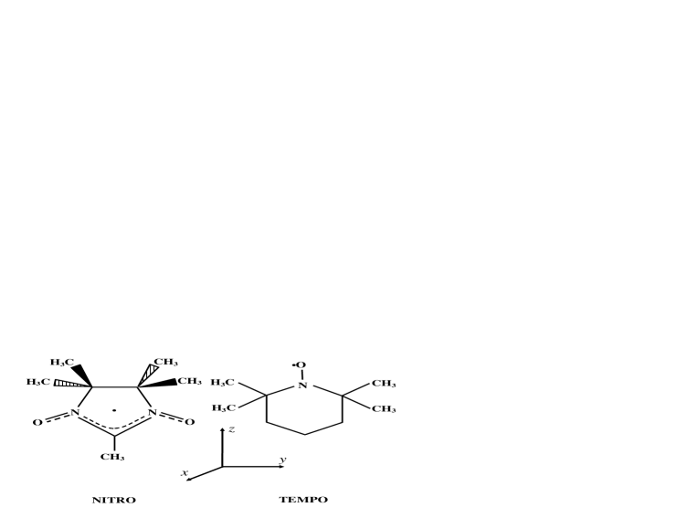
Figure 3: NITRO and TEMPO radicals.

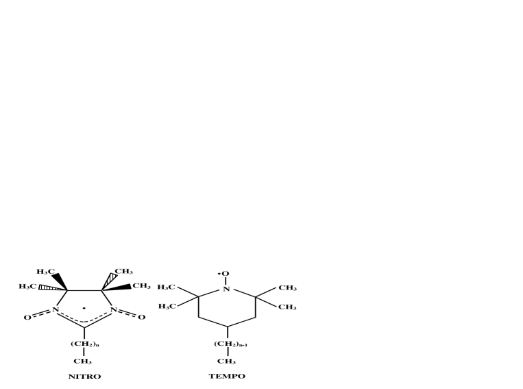
Figure 4: NITRO and TEMPO radicals with $CH_{2}$ tails ($n=1,2$).

As the promising candidates for qubits in SAM of organic radicals we selected two well-known stable organic radicals, namely methyl group substituted nitronyl nitroxide (NITRO) and 2,2,6,6-tetramethylpiperidin (TEMPO) (see Fig. 3), which form stable organic crystals and already have applications in material sciences as well as biochemistry. Both chosen radicals possess one unpaired electron and therefore each radical can be recognized as a single qubit. The geometry of NITRO and TEMPO radicals used in calculations of electronic g-tensors and of dipole-dipole interaction tensor D have been obtained by performing geometry optimization of single radical in 6-311G(d,p) basis set 6311g at the B3LYP becke ; lyp ; b3hyb level . All geometry optimizations have been carried out in Gaussian-98 program gaus98 . Apart from optimizing geometries of NITRO and TEMPO radicals we performed geometry optimization of the NITRO and TEMPO radicals derivatives with ${\rm(CH_{2})_{n}}$ tails (see Fig. 4). The ${\rm(CH_{2})_{n}}$ groups were added to radicals in order to simulate conventional structure of the compounds used in formation of SAM, which usually feature long ${\rm(CH_{2})}$ groups or similar tails. Obtained structures of NITRO and TEMPO radicals with ${\rm(CH_{2})_{n}}$ tails have been used to investigate influence of the tails on the properties of the NITRO and TEMPO derivatives compared to free NITRO and TEMPO radicals and allowed us to estimate feasibility of the NITRO and TEMPO radicals usage as basic building blocks of the spin arrays in SAM.

Calculations of electronic g-tensors for NITRO and TEMPO radicals as well as their derivatives with ${\rm(CH_{2})}$ tails have been carried out using BP86 exchange–correlation functional becke ; pw86 , which gives accurate results for organic radicals. In all calculations of g-tensors we employed IGLO-II basis set iglo2 especially designed for evaluation of magnetic properties. In order to estimate influence of the ${\rm(CH_{2})_{n}}$ (n=1,2) tails, which usually added to radicals in order to enable formation of SAM, on the electronic g-tensors of the radicals we carried out electronic g-tensors calculations for single NITRO and TEMPO radicals (see Fig. 3) as their derivatives with ${\rm(CH_{2})_{n}}$ tails (see Fig. 4).

Calculations of the dipole-dipole interaction tensor between two NITRO or two TEMPO radicals have been performed using previously described point dipole and “point dipole–spin density” approaches varying the distance between radicals, $a$, from 1 nm to 2 nm. Single radicals optimized geometries have been employed in calculations using “point dipole–spin density” approach. All calculations have been performed at the B3LYP level using Duning’s double zeta basis set dz , which allow adequate description of the electron density distribution in investigated radicals. In calculations of the dipole-dipole interaction tensor we limited ourselves only by investigation of the $D_{zz}$ component dependence on the distance between radicals $a$ and contrary to investigation of the electronic g-tensors do not carried out investigation of the ${\rm(CH_{2})_{n}}$ tails influence on dipole-dipole interaction tensor ${\bf D}$, as our g-tensor calculations indicated negligible influence of the ${\rm(CH_{2})_{n}}$ tails on unpaired electron density distribution in both NITRO and TEMPO radicals.

VI 6. Results and discussion

A. Electronic g-tensor

Electronic g-tensor calculations results for single NITRO and TEMPO molecules as well as their derivatives with ${\rm(CH_{2})_{n}}$ n=1,2 tails are tabulated in Table 1. 1 The results of electronic g-tensor calculations for NITRO compound with ${\rm(CH_{2})_{n}}$ tail separated for two different conformations of this compound, which differ only by orientation of the tail with one ${\rm(CH_{2})}$ unit. However, already for tail consisting of the two ${\rm(CH_{2})}$ units, there is no difference between NITRO A and NITRO B conformations due to the increased flexibility of tail, which leads geometry optimization procedure converges to same structure independently on the starting geometry. Here, we note even thought our calculations predict small radical tail rotation around C-C bonds it does not correspond to the “real” behavior of the ${\rm(CH_{2})}$ tail in SAM, as the motion of the tail is constrained by surrounding molecule tails in SAM. Now let us turn discussion from radicals geometrical structure features to their electronic g-tensors, which are one of the key quantities in our two qubit system Spin Hamiltonian.

All electronic g-tensor components, presented in Table 1,  1 are only slightly altered by addition of ${\rm(CH_{2})_{n}}$ tail chain units, suggesting small distortion of unpaired electron density in radical by such chemical modification. The electronic g-tensor shifts almost converge, and extension of the chain further from two to three ${\rm(CH_{2})}$ units changes g-shift components in range 1-5 ppm. Therefore, we conclude that electronic g-tensors of the NITRO and TEMPO radicals are only slightly affected by chemical addition of the ${\rm(CH_{2})_{n}}$ tail, which is required for growth of the SAM, i.e. both radicals preserve their properties in SAM. Selected radicals have highly anisotropic electronic g-tensor (see Table 1  1 ) with large $\Delta g_{xx}$ and $\Delta g_{yy}$ components (for orientation of the electronic g-tensor axes see Fig. 1). Only $\Delta g_{zz}$ is small, and therefore along this axis we have molecular g-tensor component close to the free electron g-factor. The large anisotropy of the electronic g-tensor poses significant difficulties for the quantum computation prospective as in order to have well defined frequencies of the transitions it is essential to have fixed orientation of the electronic g-tensor principal axes with respect to the external magnetic field, i.e. radicals in SAM should be fixed in their position and rotations of the radicals with respect to their g-tensor principle axes must be restrained.

B. Dipole-dipole interaction

Dipole-dipole interaction tensor between two radicals is one of the key parameters in the spin Hamiltonian, which describes the two qubit system. We employed different approaches, namely classical point dipole approach and “point dipole–spin density” approach, for evaluation of the $D=|D_{zz}|$.The second approach as discussed previously partially accounts electron distribution in molecule and therefore results are directly dependent on the unpaired electron density localization in the molecule. Contrary, the first approach does not account for unpaired electron delocalization in radical and therefore gives the same results for all radicals. The dipole-dipole interaction dependence on the distance between radicals $a$ is plotted in Fig. 5, where results for both classical point dipole approach (denoted classical) and “point dipole–spin density” approach (denoted Nitro and Tempo for NITRO and TEMPO radicals, respectively). Quick inspection of these plots indicates a substantial influence of the unpaired electron delocalization on the $D$ value especially at the small $a$ region. Therefore, unpaired electron delocalization can not be neglected in evaluation of the ${\bf D}$ tensor and previous data, which have been used in modeling of the qubits system, obtained with classical point dipole approach should be carefully reexamined for $a$ range of the 10-15 Å. Another implication of the non-negligible contribution from unpaired electron delocalization to the dipole-dipole interaction is that orientation of the radical can influence ${\bf D}$ tensor components values. Therefore, similarly to electronic g-tensor calculations the dipole-dipole interaction modeling results suggest that the rigid fixation of the radical in SAM with specific orientation is one of the key requirements in production of SAM in order to make them useful in quantum computing.

VII 7. Conclusion

We have suggested using NITRO and TEMPO radicals as spin qubits for a quantum logical device based on SAM systems. In order to stimulate experimental implementation of our idea we have computed the components of g-tensor and dipole-dipole interaction tensor for these radicals. We have shown that adding $(CH_{2})_{n}$ tail chain does not influence significantly the radical electron g-factor. Delocalization of the electron spin in radicals influences the dipole-dipole interaction between the radicals. We suggested a scheme for detection of the entanglement between the two radicals based on the novel OSCAR technique, which has been recently used for the single-spin detection.

Table 1: Shift of the electronic g-tensor components on ${\rm(CH_{2})_{n}}$ chain in nitronyl-nitroxide and TEMPO radicals. ^a,b

		NITRO A				NITRO B				TEMPO
Tail		—	${\rm CH_{2}}$	${\rm(CH_{2})_{2}}$		—	${\rm CH_{2}}$	${\rm(CH_{2})_{2}}$		—	${\rm CH_{2}}$	${\rm(CH_{2})_{2}}$
$\Delta g_{11}$		63	56	51		63	59	51		27	58	86
$\Delta g_{22}$		8922	8905	8882		8922	8889	8838		7289	7278	7245
$\Delta g_{33}$		4206	4203	4206		4206	4203	4206		3945	3989	3791

^a Electronic g-tensor RDFT-LR calculations performed using BP86 exchange–correlation functional in Huz-II basis set. ^b Electronic g-tensor shifts are in ppm.

Figure 1: Two spins ${\vec{S}}(1)$ and ${\vec{S}}(2)$ separated by the distance $a$. The external magnetic field ${\vec{B}}(y)$ is oriented in the positive $z$-direction and has a gradient in the $y$-direction. In the ground state, shown in the figure, the spins point in the negative $z$-direction, $G=|\partial B_{z}/\partial y|$.

Figure 2: The diagram of the energy levels for the two qubit system.

Figure 5: Dependence of the parameter $D$ on the distance between two radicals in the spin group (1 - two interacting TEMPO radicals, 2 - two interacting NITRO radicals, 3 - two interacting point dipoles.

References

- (1) J. Chen, M.A. Reed, A.M. Rawlett, and J.M. Tour, SCIENCE, 286, 1550 (1999).
- (2) G. P. Berman, V. I. Tsifrinovich and D. L. Allara, Phys. Rev. B 66, 193406 (2002).
- (3) A. Tamulis, V.I. Tsifrinovich, S. Tretiak, G.P. Berman, and D.L. Allara, quant-ph/0307136.
- (4) D. Rugar, R. Budakian, H.J. Mamin, and B.W. Chui, NATURE, 430, 329 (2004).
- (5) G.P. Berman, F. Borgonovi, and V.I. Tsifrinovich, Quantum Information and Computation, 4, 102 (2004).
- (6) Z. Rinkevicius, L. Telyatnyk, P. Sałek, O. Vahtras and H. Ågren, J. Chem. Phys. 119, 10489 (2003).
- (7) O. L. Malkina, J. Vaara, B. Schimmelpfennig, M. Munzarová, V. G. Malkin and M. Kaupp, J. Am. Chem. Soc. 122, 9206 (2000).
- (8) F. Neese, J. Chem. Phys. 115, 11080 (2001)
- (9) M. Kaupp, R. Reviakine, O. L. Malkina, A. Arbuznikov, B. Schimmelpfenning and V. G. Malkin, J. Computational Chem. 23, 794 (2002).
- (10) T. Helgaker, H. J. Aa. Jensen, P. Jørgensen, J. Olsen, K. Ruud, H. Ågren, A. A. Auer, K. L. Bak, V. Bakken, O. Christiansen, S. Coriani, P. Dahle, E. K. Dalskov, T. Enevoldsen, B. Fernandez, C. Hättig, K. Hald, A. Halkier, H. Heiberg, H. Hettema, D. Jonsson, S. Kirpekar, R. Kobayashi, H. Koch, K. V. Mikkelsen, P. Norman, M. J. Packer, T. B. Pedersen, T. A. Ruden, A. Sanchez, T. Saue, S. P. A. Sauer, B. Schimmelpfennig, K. O. Sylvester-Hvid, P. R. Taylor, and O. Vahtras, DALTON, a molecular electronic structure program, Release 1.2 (2001). See http://www.kjemi.uio.no/software/dalton/dalton.html.
- (11) B. A. Hess, C. M. Marian, U. Wahlgren and O. Gropen, Chem. Phys. Lett. 251, 365 (1996).
- (12) R. Krishnan, J. S. Binkley, R. Seeger and J. A. Pople, J. Chem. Phys. 72, 650 (1980).
- (13) A.D. Becke, Phys. Rev. A 38, 3098 (1988).
- (14) C. Lee, W. Yang and R.G. Parr, Phys. Rev. B, 37, 785 (1988).
- (15) A. D. Becke, J. Chem. Phys. 98, 5648 (1993).
- (16) M. J. Frisch, G. W. Trucks, H. B. Schlegel, G. E. Scuseria, M. A. Robb, J. R. Cheeseman, V. G. Zakrzewski, J. A. Montgomery, Jr., R. E. Stratmann, J. C. Burant, S. Dapprich, J. M. Millam, A. D. Daniels, K. N. Kudin, M. C. Strain, O. Farkas, J. Tomasi, V. Barone, M. Cossi, R. Cammi, B. Mennucci, C. Pomelli, C. Adamo, S. Clifford, J. Ochterski, G. A. Petersson, P. Y. Ayala, Q. Cui, K. Morokuma, D. K. Malick, A. D. Rabuck, K. Raghavachari, J. B. Foresman, J. Cioslowski, J. V. Ortiz, A. G. Baboul, B. B. Stefanov, G. Liu, A. Liashenko, P. Piskorz, I. Komaromi, R. Gomperts, R. L. Martin, D. J. Fox, T. Keith, M. A. Al-Laham, C. Y. Peng, A. Nanayakkara, C. Gonzalez, M. Challacombe, P. M. W. Gill, B. Johnson, W. Chen, M. W. Wong, J. L. Andres, C. Gonzalez, M. Head-Gordon, E. S. Replogle, and J. A. Pople, Gaussian 98, Revision A.7 (Gaussian, Inc., Pittsburgh PA, 1998).
- (17) J. P. Perdew, Phys. Rev. B 33, 8822 (1986).
- (18) W. Kutzelnigg, U. Fleischer, and M. Schindler, in NMR Basic Principles and Progress, Vol. 23, edited by P. Diehl, E. Fluck, H. Günther, R. Kosfeld, and J. Seelig (Springer, Heidelberg, 1990), p. 165.
- (19) T. H. Dunning, Jr., J.Chem.Phys. 53, 2823 (1970).