Analyses of reflection and transmission at moving potential step

Abstract

The reflection and transmission of wave functions at a potential step is a well-known issue in a textbook of quantum mechanics. We studied the reflection and transmission characteristics analytically when the potential step is moving at a constant velocity $v$ in the same direction as an incident wave function by means of solving the time-dependent Schrödinger equation. As for an infinite potential step, it is known that group velocity is the same as the moving velocity of the potential step. We found two interesting results when the potential step has a finite height of $V_{0}$. The transmission occurs when the kinetic energy of incident wave function is larger than the effective potential hight of $\left(\sqrt{\frac{m}{2}}v+\sqrt{V_{0}}\right)^{2}$. The other result is that the reflectivity depends on $x$, which derives from the interference between the incident and the reflected wave functions.

I Introduction

The reflection and transmission of wave functions at a potential step is one of the most fundamental issue in general textbooks on quantum mechanics Schiff (1981). It is surely a basic concept of electron tunneling in nanoelectronics. Actually the electron tunneling has been applied to scanning tunneling microscopy, Josephson devices, superlattices, resonant tunneling devices, and so on Wolf (1985). When we calculate the reflectivity and transmissivity, we solve the time-independent Shrödinger equation to obtain the wave functions of a stationary state, and then calculate the ratio of the reflected and the transmitted probability current density to that of incident flux. In these calculations, a boundary condition is not varied with time.

We are interested in the state where the boundary condition depends on time. This kind of problem is of interest for instance in expanding force fields Berry and Klein (1984), or in the evolution of metastable states in the early universe that is an interesting issue in cosmology Lee and Ho . We treat in this article two problems of a finite or an infinite potential step moving with a constant velocity. These problems are the most basic concepts of quantum issues where boundary conditions are dependent on time.

II Infinite potential step

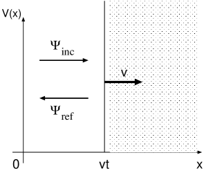
Figure 1: The schematic diagram of a infinite potential step.

We solve the time-dependent Schrödinger equation in one dimension as

$$i\hbar\frac{\partial\Psi}{\partial t}=-\frac{\hbar^{2}}{2m}\frac{\partial^{2}\Psi}{\partial x^{2}},$$ (1)

with a boundary condition that an infinite potential step is located at $x=vt$ as shown in FIG. 1. It is because we can not use the time-independent Schrödinger equation with the boundary conditions that depend on time. Although this analysis has been previously reported by Luan et al. Luan and Kao , we describe the essence of their theory here for the better understanding of the finite potential analysis described in the next section. We assume a general solution to be

$$\Psi(x,t)=Ae^{i(k_{1}x-\omega_{1}t)}+Be^{i(k_{2}x-\omega_{2}t)},$$ (2)

where the two terms correspond to an incident and a reflected wave function, respectively. We should pay attention to $\frac{\hbar k_{1}}{m}\gg v$ that means the semi-classical point of view. The solution (2) satisfies the Schrödinger equation (1) only when

$$\omega_{1}=\frac{\hbar}{2m}k_{1}^{2}~{}~{}{\textrm{and}}~{}~{}\omega_{2}=\frac{\hbar}{2m}k_{2}^{2}.$$ (3)

We consider two boundary conditions here. One condition is that the wave function is zero (i.e. $A+B=0$) at the boundary. The other condition should be that the first derivative of the wave function is also zero at the boundary. Since the position of the boundary is a function of $t$, the latter boundary condition can not be used in the same manner as the boundary is fixed with time. We then give an alternative boundary condition that the phases of the incident and the reflected wave functions at the boundary are the same i.e. $k_{1}v-w_{1}=k_{2}v-w_{2}$. This condition comes into

$$k_{2}=-k_{1}+\frac{2mv}{\hbar},$$ (4)

with the help of the equation (3). The expression (4) can be well understood as a perfect elastic collision in a classical mechanics. From these results, we can obtain the probability density:

$$|\Psi|^{2}=4|A|^{2}\sin^{2}\left[\left(k_{1}-\frac{mv}{\hbar}\right)\left(x-vt\right)\right].$$ (5)

On the other hand, the probability current density $j$ becomes

$$j = \frac{\hbar}{2mi}\left(\Psi^{*}\frac{\partial\Psi}{\partial x}-\frac{\partial\Psi^{*}}{\partial x}\Psi\right)$$ (6)

$$= 4v|A|^{2}\sin^{2}\left(k_{1}-\frac{mv}{\hbar}\right)\left(x-vt\right).$$

A group velocity can be calculated by dividing the probability current density by the probability density. We find that the group velocity is equal to $v$.

III Finite potential step

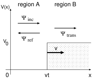
Figure 2: The schematic diagram of a finite potential step.

We consider the other case that the potential step is as high as $V_{0}$ as shown in FIG. 2. The boundary is moving toward $+x$ with a speed of $v$. We should treat the two kinds of Schrödinger equations in the two regions A and B as

$$i\hbar\frac{\partial\Psi_{A}}{\partial t}=-\frac{\hbar^{2}}{2m}\frac{\partial^{2}\Psi_{A}}{\partial x^{2}}~{}~{}\left(x\leq vt:~{}\textrm{region~{}A}\right)\\$$ (7)

$$~{}~{}{\textrm{and}}~{}~{}i\hbar\frac{\partial\Psi_{B}}{\partial t}=-\frac{\hbar^{2}}{2m}\frac{\partial^{2}\Psi_{B}}{\partial x^{2}}+V_{0}\Psi_{B}~{}~{}\left(vt<x:~{}\textrm{region~{}B}\right),$$ (8)

because transmitted wave function can exist in this case. We assume general solutions in the two regions as

$$\Psi_{A}(x,t)=Ae^{i(k_{1}x-\omega_{1}t)}+Be^{i(k_{2}x-\omega_{2}t)}$$ (9)

$$~{}~{}{\textrm{and}}~{}~{}\Psi_{B}(x,t)=Ce^{i(k_{3}x-\omega_{3}t)}.$$ (10)

The first and the second terms in (9) correspond to an incident and a reflected wave function, respectively. The solution (10) corresponds to the transmitted wave function. We can obtain

$$\omega_{1}=\frac{\hbar}{2m}k_{1}^{2},~{}~{}\omega_{2}=\frac{\hbar}{2m}k_{2}^{2}~{}~{}{\textrm{and}}~{}~{}\omega_{3}=\frac{\hbar}{2m}k_{3}^{2}+\frac{V_{0}}{\hbar}$$ (11)

in the same way as the infinite potential step. We give two boundary conditions as

$$A+B=C$$ (12)

$$~{}~{}{\textrm{and}}~{}~{}k_{1}v-\omega_{1}=k_{2}v-\omega_{2}=k_{3}v-\omega_{3}.$$ (13)

The condition (13) derives from our assumption that the phase of each wave function is the same. From the relationship of (13) we can obtain the expressions:

$$k_{2}=-k_{1}+\frac{2mv}{\hbar}$$ (14)

$$~{}~{}{\textrm{and}}~{}~{}k_{3}=\frac{mv}{\hbar}+\sqrt{\left(k_{1}-\frac{mv}{\hbar}\right)^{2}-\frac{2mV_{0}}{\hbar^{2}}}.$$ (15)

When we substitute $v=0$ in the expressions (14) and (15), we can arrive at the well-known expressions for the potential step without moving. The expression (14) describes the perfect elastic reflection at the boundary similarly with the case of the infinite potential step. In order to investigate the expression (15), we should understand $k_{1}$ should be greater than $mv/\hbar$. This is required for the collision of the incident wave function at the boundary. We should pay attention to another critical point where the sign of the expression inside the root in (15) is changed;

$$k_{1}=\frac{mv}{\hbar}+\frac{\sqrt{2mV_{0}}}{\hbar}.$$ (16)

If the $k_{1}$ is greater than (16), the transmitted wave function is oscillating, otherwise is of a damping oscillation. The critical wave number is dependent on $v$. The first term in (16) is the effect of the moving of the potential step. We can understand that $\left(\sqrt{\frac{m}{2}}v+\sqrt{V_{0}}\right)^{2}$ is the effective potential height of the step.

III.1 The case I ($k_{1}>(\ref{eq-16})$)

We consider the case that the transmitted wave function is oscillating. Using the expressions (11), (14) and (15), the probability density in the two regions are calculated as

$$|\Psi_{A}|^{2} = |A|^{2}+|B|^{2}+A^{*}Be^{-i\left\{2\left(k_{1}-\frac{mv}{\hbar}\right)\left(x-vt\right)\right\}}$$ (17)

$$+ AB^{*}e^{i\left\{2\left(k_{1}-\frac{mv}{\hbar}\right)\left(x-vt\right)\right\}}$$

$$~{}~{}{\textrm{and}}~{}~{}|\Psi_{B}|^{2}=|C|^{2},$$ (18)

where asterisks stand for the complex conjugate. On the other hand, the probability current densities in the two regions become

$$j_{A} = \frac{\hbar}{m}\left[\left(k_{1}|A|^{2}+k_{2}|B|^{2}\right)\right.$$ (19)

$$+ \left.\frac{mv}{\hbar}\left\{AB^{*}e^{i\left\{2\left(k_{1}-\frac{mv}{\hbar}\right)\left(x-vt\right)\right\}}\right.\right.$$

$$+ \left.\left.A^{*}Be^{-i\left\{2\left(k_{1}-\frac{mv}{\hbar}\right)\left(x-vt\right)\right\}}\right\}\right]$$

$$~{}~{}{\textrm{and}}~{}~{}j_{B}=\frac{\hbar}{m}k_{3}|C|^{2}.$$ (20)

The expression (19) describes the sum of the incident and reflected probability current densities and the (20) the transmitted one. The complex coefficients of $A$, $B$, and $C$ can be generally expressed in the form of

$$A=ae^{i\theta_{a}},~{}~{}B=be^{i\theta_{b}}~{}~{}{\textrm{and}}~{}~{}C=ce^{i\theta_{c}},$$ (21)

respectively, where all variables are real values. We can describe the boundary condition of (12) in the other form as

$$a+b=c~{}~{}{\textrm{and}}~{}~{}\theta_{a}=\theta_{b}=\theta_{c}.$$ (22)

Since $|\Psi_{A}|^{2}$ and $|\Psi_{B}|^{2}$ are continuous at $x=vt$, we obtain $(a+b)^{2}=c^{2}$ . On the other hand, the continuity condition of the probability current density gives the relationship of

$$k_{1}a^{2}+k_{2}b^{2}+\frac{2mv}{\hbar}ab=k_{3}c^{2},$$ (23)

and we find the two expressions:

$$\frac{b}{a}=\frac{k_{1}-k_{3}}{k_{1}+k_{3}-\frac{2mv}{\hbar}}$$ (24)

$$~{}~{}{\textrm{and}}~{}~{}\frac{c}{a}=\frac{2k_{1}-\frac{2mv}{\hbar}}{k_{1}+k_{3}-\frac{2mv}{\hbar}},$$ (25)

that arrive at well-known results when the potential step does not move i.e. $v=0$. By the way, the probability current density in the region A (the expression (19)) can be separated in the two components of the incident and the reflected current densities as follows:

$$j_{inc}=\frac{\hbar}{m}k_{1}|A|^{2}$$ (26)

$$~{}~{}{\textrm{and}}~{}~{}j_{ref} = -\frac{\hbar}{m}\left[k_{2}|B|^{2}\right.$$ (27)

$$+ \left.\frac{mv}{\hbar}\left\{AB^{*}e^{i\left\{2\left(k_{1}-\frac{mv}{\hbar}\right)\left(x-vt\right)\right\}}\right.\right.$$

$$+ \left.\left.A^{*}Be^{-i\left\{2\left(k_{1}-\frac{mv}{\hbar}\right)\left(x-vt\right)\right\}}\right\}\right].$$

We finally obtain reflectivity and transmissivity by dividing $J_{ref}$ and $J_{B}$ by $J_{inc}$:

$$R=\frac{-k_{2}b^{2}-\frac{2mv}{\hbar}ab\cos\left\{2\left(k_{1}-\frac{mv}{\hbar}\right)\left(x-vt\right)\right\}}{k_{1}a^{2}}$$ (28)

$$~{}~{}{\textrm{and}}~{}~{}T=\frac{k_{3}c^{2}}{k_{1}a^{2}}.$$ (29)

Using the expressions (28) and (29), $R+T$ can be confirmed to be unity at the boundary.

We can easily verify our results by considering the case of $v=0$. The expressions (24) and (25) arrive at well-known results when $v=0$. The expression of $T$ is the same as the one where $v=0$. It is interesting that $R$ depends on $x$ and $t$. The fact derives from the interference effect of the incident and reflected wave functions. The interference can occur only when the potential step is moving. It is caused by the difference between the absolute values of $k_{1}$ and $k_{2}$. We suppose that the effect can be applied to quantum wave interference devices.

III.2 The case II ($k_{1}<(\ref{eq-16})$)

We consider the case that $k_{1}$ is smaller than the critical wave number of (16). We pointed out that transmitted wave function should be of a damping oscillation scheme. The $k_{1}$ should be larger than $mv/\hbar$ in order that the group velocity of the incident wave function is larger than $v$ to reach the boundary. We assume that $k_{1}$ is far large than $mv/\hbar$ from the semi-classical point of view. The different point from the case I is that the $k_{3}$ becomes an complex number as

$$k_{3}=\gamma+i\beta,~{}~{}{\textrm{where}}~{}~{}\gamma=\frac{mv}{\hbar}$$

$$~{}~{}{\textrm{and}}~{}~{}\beta=\sqrt{\frac{2mV_{0}}{\hbar^{2}}-\left(k_{1}-\frac{mv}{\hbar}\right)^{2}}>0,$$ (30)

and then we obtain $\omega_{3}$ using the relationship (11),

$$\omega_{3}=\sigma+iv\beta,$$

$${\textrm{where}}~{}~{}\sigma=\frac{\hbar}{2m}\left(k_{1}^{2}-\frac{2mv}{\hbar}k_{1}+\frac{2m^{2}v^{2}}{\hbar^{2}}\right).$$ (31)

By substituting (30) and (31) for the expression (10), we obtain the wave function in the region B as

$$\Psi_{B}=Ce^{-\beta\left(x-vt\right)+i\left(\gamma x-\sigma t\right)}.$$ (32)

Therefore, the probability density and the probability current density in the region B are expressed as

$$|\Psi_{B}|^{2}=|C|^{2}e^{-2\beta\left(x-vt\right)}$$ (33)

$$~{}~{}{\textrm{and}}~{}~{}j_{B}=\frac{\hbar}{m}|C|^{2}\gamma e^{-2\beta\left(x-vt\right)}$$ (34)

Dividing (34) by (33) shows us that the group velocity is $v$. On the basis of the same discussion of (21) and (22) before, we can obtain $(a+b)^{2}=c^{2}$ also in this case, and draw the relationship of

$$k_{1}a^{2}+k_{2}b^{2}+\frac{2mv}{\hbar}ab=\gamma c^{2}$$ (35)

in stead of (23). Using $a+b=c$, we get simple relations of

$$\frac{b}{a}=1,~{}~{}\frac{c}{a}=2.$$ (36)

We substitute (36) for (28) and (29) to arrive at

$$R=1-4\frac{mv}{\hbar k_{1}}\cos^{2}\left(k_{1}-\frac{mv}{\hbar}\right)\left(x-vt\right)$$ (37)

$$T=4\frac{mv}{\hbar k_{1}}e^{-2\beta\left(x-vt\right)}.$$ (38)

We can confirm easily that $R+T=1$ at the boundary and that $R=1$ and $T=0$ if $v=0$. The semi-classical condition denoted in the previous section plays an important role here. It ensures that $T$ is less than unity.

IV Conclusion

We investigated the characteristics of the wave function and probability current density in a system with the potential step moving toward $+x$ direction at a constant velocity $v$. Since the position of the boundary depends on time, we solve the time-dependent Schrödinger equation in one dimension. We used our boundary condition that the phases of the wave functions at the boundary are the same instead of ordinary condition that the first derivative of the wave function is the same at the boundary. We found the relation between the wave numbers of the incident and the reflected wave functions. The absolute value of the wave number is changed when the wave function is reflected at the boundary. When the potential step is finite, the wave function can be transmitted if the energy of the incident wave function is larger than the effective potential height that is depend on $v$.

References

• Schiff (1981) L.Β I. Schiff, Quantum mechnics (McGraw-Hill, 1981).
• Wolf (1985) E.Β L. Wolf, Principles of Electron Tunneling Spectroscopy (Oxford Univ. Press, 1985).
• Berry and Klein (1984) M.Β V. Berry and G.Β Klein, J. Phys. A: Math. Gen. 17, 1805 (1984).
• (4) C.-C. Lee and C.-L. Ho, eprint quant-ph/0404149.
• (5) P.-G. Luan and Y.-M. Kao, eprint quant-ph/0203054.