Coherent control of trapped ions using off-resonant lasers

Abstract

In this paper we develop a unified framework to study the coherent control of trapped ions subject to state-dependent forces. Taking different limits in our theory, we can reproduce two different designs of a two-qubit quantum gate —the pushing gate Cirac and Zoler (2000) and the fast gates based on laser pulses from Ref. García-Ripoll et al. (2003)—, and propose a new design based on continuous laser beams. We demonstrate how to simulate Ising Hamiltonians in a many ions setup, and how to create highly entangled states and induce squeezing. Finally, in a detailed analysis we identify the physical limits of this technique and study the dependence of errors on the temperature.

I Introduction

Trapped ions constitute one of the most promising systems to implement a scalable quantum computer Levi (2003). In such a computer, information is stored in long-lived atomic states, and a universal set of gates is obtained by manipulating these states with lasers, and entangling the ions via the vibrational modes Cirac and Zoler (2000). During the last years we have seen experimental demonstrations of various two–qubit gates Monroe et al. (1995); DeMarco et al. (2002); Leibfried et al. (2003); Schmidt-Kaler et al. (2003), and it remains to implement a robust scheme for scalability. Current visions of a scalable computer are based on the idea of moving the ions out of their storage area (or quantum memory) and make them interact in pairs, performing two-qubit gates Cirac and Zoler (2000); Kielpinski et al. (2002). Basic steps towards the experimental implementation of this idea have been already demonstrated. Rowe et al. (2002).

However, outside quantum computing there are other promising areas in which trapped ions may be of use. On the one hand, there is a great interest in preparing highly entangled or squeezed states, which can be used both for metrology Wineland et al. (1992, 1994), or — in a more fundamental fashion — to characterize their decoherence properties. The entanglement of ions is covered in a variety of theoretical papers Steinbach and Gerry (1998); Mølmer and Sørensen (1999); Sørensen and Mølmer (2000); Unanyan and Fleischhauer (2003), and it has been experimentally demonstrated for small systems Turchette et al. (1998); Sackett et al. (2000); Meyer et al. (2001). On the other hand, it has also been suggested that ion traps can be used to simulate a various spin Hamiltonians, ranging from local to long-range interactions Porras and Cirac (2004); Barjaktarevic et al. .

In all of these tasks —quantum computing, creation of entanglement and quantum simulation—, the goal is to induce some unitary evolution on the internal state of the ions, which is used to store the information. For instance, in the case of quantum computing it suffices to realize a phase gate between two ions

$$U_{ph}(T)=e^{i\pi\sigma^{z}_{1}\sigma^{z}_{2}/4},$$ (1)

while in the case of quantum simulation we want a more general evolution

$$U(T)=e^{i\left(\sum_{i,j}\vec{\sigma}_{i}J_{ij}\vec{\sigma}_{j}+\sum_{i}\vec{B}_{i}\vec{\sigma}_{i}\right)T},$$ (2)

where the matrices $J_{ij}$ and the vectors $\vec{B}_{i}$ determine the spin Hamiltonian that we want to simulate. Since the real interaction between the ions is described by more complicated Hamiltonians [See Eq. (3) below], any of these transformations is an effective one, realized after influencing the dynamics of the ions with external fields. This process, in which we dynamically modify the parameters of the system —Rabi frequencies, detunings, magnetic fields, etc—, in order to achieve a well defined target operation, is called Coherent Quantum Control.

While coherent control has been implicit in any proposal for quantum computing Cirac and Zoller (1995); Poyatos et al. (1998); Sørensen and Mølmer (1999); Cirac and Zoler (2000); Sørensen and Mølmer (2000); Jonathan et al. (2000); James (2000); Milburn et al. (2000); García-Ripoll et al. (2003); Duan ; Staanum et al. (2004) and quantum simulation Porras and Cirac (2004); Barjaktarevic et al. with ion traps, the development of these schemes of control relied always on the intuition of the researcher and on a clever choice of approximations. In this work we show that many of these schemes can be translated into a unified framework based on state dependent forces and tunable traps. As characteristic examples, we will show how to implement the pushing gate Cirac and Zoler (2000) and the fast gates based on laser pulses from Ref. García-Ripoll et al. (2003). We will also propose an alternative and more general model of fast gate based on continuous off-resonant lasers. As further applications, we demonstrate how to induce collective $H=(\sum_{i}\sigma^{z}_{i})^{2}$ and nearest neighbor $H=\sum_{i}J\sigma^{z}_{i}\sigma^{z}_{i+1}$ Ising interactions, and use them to produce squeezing, and generate cluster and GHZ states of up to 30 atoms within a extremely short time, $T={\cal O}(1/\omega)$, where $\omega$ is the frequency of the ion trap.

Furthermore, within this unified framework we can address important requirements of all these coherent processes. Namely they should: (i) be independent of temperature (so that one does not need to cool the ions to their ground state after they are moved to or from their storage area); (ii) require no addressability (to allow the ions to be as close as possible during the gate so as to strengthen their interaction), and (iii) be fast (in order to minimize the effects of decoherence during the gate, and to speed up the computation). All of these requirements can be formulated as constraints of the control problem, and as we will see below, they can be easily solved. Last but not least, we study the scaling of resources as we try to make our control faster and answer the question of what is the ultimate limit for the speed of our quantum gates or entangling processes, which is shown to be determined both by dissipation and non-harmonic contributions to the restoring forces.

The paper is organized as follows. In Sec. II we develop the formalism to study our system. First of all, we introduce the Hamiltonian for any number of ions subject to state dependent forces and quasi-1D confinement, and derive the harmonic approximation and the normal modes. Then, we show how to implement a unitary transformation, $U=\exp[i\phi(\{\sigma^{z}_{i}\})]$, made of robust geometrical, while leaving the motional state unchanged. In Sec. III we apply our methods to quantum computing in two-qubit setups. We demonstrate how to recover previous designs of a phase gate, including the adiabatic pushing gate Cirac and Zoler (2000) and the fast gate based on $\pi/2$ laser pulses that kick the ions García-Ripoll et al. (2003). Most important, since the generation of perfect and very short laser pulses is a difficult task, we design an arbitrarily fast quantum gate based on continuous laser sources. In Sec. IV we study the coherent control of many-ion setups. We prove that arbitrary spin interactions of the type (2) can be simulated with the appropriate time-dependent forces, and develop a numerical method to find them. As applications, we demonstrate numerically the creation of squeezed, cluster and GHZ states of up to 30 ions in a very short time. Sec. V focuses on the study of errors. First of all we introduce a model for dissipation on the vibrational degrees of freedom. Next, we solve this model exactly and analyze the fidelity of the effective unitary operations (1)-(2). We prove that for a perfect control and no dissipation our scheme is insensitive to temperature. Furthermore, the errors due to interaction with the environment can be computed and optimized using the same tools of quantum control as in Sec. III-IV. Finally, we study the errors due to anharmonic terms in the interaction and show that both this and dissipation set an upper bound on the speed of the gate. In Sec. VI we summarize our results and offer perspectives for future work.

II Theory

II.1 Normal modes

As mentioned before, this paper studies a set of $N$ ions, in an essentially one-dimensional confinement and subject to some external forces. Our model Hamiltonian is

$$H=\sum_{i}\left[\frac{p_{i}^{2}}{2m}+V_{e,i}(x_{i})-F_{i}(t)x_{i}\right]+\sum_{i<j}\frac{e^{2}}{4\pi\epsilon_{0}}\frac{1}{|x_{i}-x_{j}|}.$$ (3)

In this equation, $V_{e,k}$ is the trapping potential that confines the $k$-th ion, and it may be the same for all of them or may change from ion to ion as in the case of microtraps Cirac and Zoler (2000). The time dependent external forces are denoted by $F_{i}(t)$ and, as we will see below, they depend on the internal state of the ion, $\sigma^{z}_{i}$.

If we expand the previous energy around the equilibrium configuration without forces, given by $(\partial H/\partial x_{i})(x_{1}^{(0)},\ldots,x_{N}^{(0)})=0$ and $F_{i}=0$, we obtain a set of coupled harmonic oscillators

$$H=\sum_{i}\left[\frac{p_{i}^{2}}{2m}-F_{i}(t)x_{i}\right]+\frac{1}{2}mV_{ij}x_{i}x_{j}+E_{0}.$$ (4)

The constant $E_{0}$ is the energy of the ions at their equilibrium positions. The matrix $V$ describes the restoring forces: it is symmetric, positive definite and it can decomposed as $V=M\Omega^{2}M^{t}$, with a positive diagonal matrix of frequencies, $\Omega_{kl}=\omega_{k}\delta_{kl}$, and an orthogonal transformation ($MM^{t}=M^{t}M=\mathbb{I}$). Using this canonical transformation to define the normal modes $x_{i}=\sum_{k}M_{ik}Q_{k}$, $p_{i}=\sum_{k}M_{ik}P_{k}$, we arrive at the Hamiltonian

$$H=\sum_{k}\left[\frac{P_{k}^{2}}{2m}+\frac{1}{2}m\omega_{k}^{2}Q_{k}^{2}-\sum_{i}F_{i}M_{ik}Q_{k}\right].$$ (5)

It is now useful to write this Hamiltonian in dimensionless form, using the characteristic length of the oscillators, $\alpha_{k}=(\hbar/m\omega_{k})^{1/2}$, so that $P_{k}=\hbar\tilde{P}_{k}/\alpha_{k}$ and $Q_{k}=\alpha_{k}\tilde{Q}_{k}$, $\tilde{M}_{ik}=M_{ik}\alpha_{k}$. With this we arrive to

$$H=\sum_{k}\left[\frac{1}{2}\hbar\omega_{k}\left(\tilde{P}_{k}^{2}+\tilde{Q}_{k}^{2}\right)-\sum_{i}F_{i}\tilde{M}_{ik}\tilde{Q}_{k}\right],$$ (6)

or, using of Fock operators, $a_{k}\equiv(\tilde{Q}_{k}+i\tilde{P}_{k})/\sqrt{2}$,

$$H=\sum_{k}\left[\hbar\omega_{k}\left(a_{k}^{\dagger}a_{k}+\tfrac{1}{2}\right)-\sum_{i}\frac{F_{i}\tilde{M}_{ik}}{\sqrt{2}}(a_{k}^{\dagger}+a_{k})\right].$$ (7)

II.2 Robust phases

We will now demonstrate how to obtain a robust phase by applying forces to a harmonic oscillator. Let us begin with the toy model

$$H=\hbar\omega a^{\dagger}a-f(t)\tfrac{1}{\sqrt{2}}(a^{\dagger}+a).$$ (8)

When integrating the Schrödinger equation associated with this Hamiltonian, it will convenient to use the overcomplete basis of coherent states

$$|z\rangle:=e^{-|z|^{2}/2}\sum_{n}\frac{z^{n}}{\sqrt{n!}}|n\rangle=:|Q+iP\rangle.$$ (9)

Under the Hamiltonian (8), the coherent states behave somehow like classical particles in phase space, because their center, given by $\langle Q\rangle$ and $\langle P\rangle$, follows a classical trajectory, while the width of these wavepackets, given by the uncertainty of $Q$ and $P$, remains fixed.

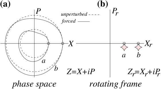
Figure 1: Trajectories on phase space of a coherent wavepacket subject to a single forced harmonic oscillator, $H=\omega a^{\dagger}a+F\sin(2t)(a+a^{\dagger})$. In Fig. (a) we plot the usual phase space trajectories, $\langle a\rangle=\langle X+iP\rangle/\sqrt{2}$, without forcing (dashed) and with F=0.1 (solid), for two initial conditions. In Fig. (b) we plot the same, but on a rotating frame of reference, $\langle a\rangle=\langle e^{-i\omega t}(X_{r}+iP_{r})\rangle/\sqrt{2}$.

More precisely, for an initial coherent state, $|\psi(0)\rangle=|z_{0}\rangle$, the solution to the Schrödinger equation $i\hbar\dot{\psi}=H(t)\psi$ is given also by a coherent state $|\psi(t)\rangle=e^{i\phi(t)}|z(t)\rangle$, whose phase and position satisfy

$$\frac{dz}{dt} = -i\omega z+i\tfrac{1}{\sqrt{2}\hbar}f(t),$$ (10a)

$$\frac{d\phi}{dt} = \tfrac{1}{2\sqrt{2}\hbar}f(t)(\bar{z}+z).$$ (10b)

The first equation has a solution,

$$z(t)=e^{-i\omega t}\left[z_{0}+\tfrac{i}{\sqrt{2}\hbar}\int_{0}^{t}d\tau\,e^{i\omega\tau}f(\tau)\right],$$ (11)

that results from composing a displacement with a rotation of angular speed $\omega$. Using the rotating phase-space coordinates, $z_{r}:=e^{i\omega t}z=:Q_{r}+iP_{r}$, we get rid of the motion due to the unforced harmonic oscillators and find

$$\frac{dz_{r}}{dt} = ie^{i\omega\tau}f(\tau)/\hbar\sqrt{2},$$ (12a)

$$\frac{d\phi}{dt} = \mathrm{Im}\,\frac{dz_{r}}{dt}\bar{z}_{r}=\frac{dP_{r}}{dt}Q_{r}-\frac{dQ_{r}}{dt}P_{r}=2\frac{dA}{dt}.$$ (12b)

The last equation means indeed that the growth of the phase is proportional to the area spanned by the coherent state as it moves through the phase space. The phase is not only geometrical in this sense, but also in the extended definition of geometrical phase given in Ref. Aharonov and Anandan (1987). Applying the formulas in the previous reference one finds that if the total phase is $\phi(t)$, and the dynamical phase is always twice the geometrical one, $\phi_{d}(t)=-2\phi_{g}(t)$, so that in the end $\phi(t)=-\phi_{g}(t)$.

In this work we are interested in this phase and on making it depend on the internal state of the particles governed by the oscillator. We want, however, neither to influence the motional state of the particles, nor to entangle internal and motional degrees of freedom. For this reason we set a time limit on the duration of the force and impose that after a fixed time $T$ the coherent wavepacket is restored to its original state

$$\int_{0}^{T}d\tau\,e^{i\omega\tau}f(\tau)=0.$$ (13)

Using this condition we derive a simple formula for the total phase

$$\phi(T) = \mathrm{Im}\int_{0}^{T}d\tau\,\tfrac{i}{\sqrt{2}\hbar}e^{i\omega\tau}f(\tau)\,\bar{z}_{r}(\tau)$$

$$= \tfrac{1}{2\hbar^{2}}\mathrm{Im}\int_{0}^{T}d\tau_{1}\int_{0}^{\tau_{1}}d\tau_{2}\,e^{i\omega(\tau_{1}-\tau_{2})}f(\tau_{1})f(\tau_{2}).$$

As a simple application, in Fig. 1 we show the phase space trajectories obtained by forcing two coherent states with a sinusoidal force, $F(t)\propto\sin(2\omega t)$, where $\omega$ is the frequency of the Harmonic oscillator. Even though looking at Fig. 1(a) the orbits of different initial conditions seem also very different, on the rotating frame of reference the enclosed area $A$ is always the same [Fig. 1(b)]. In other words, the phase $\phi$ is insensitive to the initial motional state of the system and it is thus robust. This property is of crucial importance when we seek applications to real systems that cannot be cooled to the zero phonon limit, but which thanks to Eq. (13) will pick up the same phase regardless of the temperature.

II.3 Phase of two ions

We will now apply the results from Sec. II.2 to a pair of ions. In this case there are two normal modes: the center of mass, $x_{c}=(x_{1}+x_{2})/2$, which oscillates with frequency $\omega_{c}$, and the stretch mode, $x_{s}=x_{2}-x_{1}$, which oscillates with frequency $\omega_{s}$. If the ions are stored in the same harmonic trap, $V_{e,k}(x_{k})=\frac{1}{2}m\omega^{2}x_{k}^{2}$, these frequencies are found to be incommensurate, $\omega_{c}=\omega$ and $\omega_{r}=\omega\sqrt{3}$. If we store the ions in two microtraps (or in a more complicated potential), the value of $\omega_{r}$ can be tuned from $\omega\sqrt{3}$ down to $\omega$.

If we exert a similar state dependent force on both ions, for instance by means of an off-resonance laser that induces a AC Stark shift on one of the internal state of the ions, the Hamiltonian (3) will look as follows

$$H = \hbar\omega a_{c}^{\dagger}a+\hbar\omega_{r}a_{r}^{\dagger}a_{r}-F(t)\sigma^{z}_{1}x_{1}-F(t)\sigma^{z}_{2}x_{2}$$

$$= \hbar\omega a_{c}^{\dagger}a+\hbar\omega_{r}a_{r}^{\dagger}a_{r}+F(t)(\sigma^{z}_{2}-\sigma^{z}_{1})d$$

$$- F(t)(\sigma^{z}_{1}+\sigma^{z}_{2})\frac{\alpha_{c}}{\sqrt{2}}(a_{c}+a_{c}^{\dagger})$$

$$- F(t)(\sigma^{z}_{2}-\sigma^{z}_{1})\frac{\alpha_{r}}{2\sqrt{2}}(a_{r}+a_{r}^{\dagger})$$

where $d$ is the equilibrium distance between the ions, $\alpha_{c,r}^{2}=\hbar/m\omega_{c,r}$ are the lengths of the oscillators, and $\sigma^{z}_{i}$ is an operator that has value $+1$ or $-1$ depending on whether the ion is on internal state $|+1\rangle$ or $|-1\rangle$.

Since the modes are now decoupled, we can apply the formulas of Sec. II.2 almost directly. We first obtain a pair of commensurability relations on the force

$$\int_{0}^{T}d\tau\,e^{i\omega_{c,r}\tau}F(\tau)=0,$$ (16)

which are just a generalization of Eq. (13). Next we obtain the total phase, which up to local and global contributions is

$$\phi=\sigma^{z}_{1}\sigma^{z}_{2}\int_{0}^{T}d\tau_{1}\int_{0}^{T}d\tau_{2}\,{\cal G}(\tau_{1}-\tau_{2})F(\tau_{1})F(\tau_{2})$$ (17)

where ${\cal G}(t)=\left[\frac{1}{\omega_{c}}\sin(\omega_{c}|t|)-\frac{1}{\omega_{r}}\sin(\omega_{r}|t|)\right]/2m\hbar$.

The goal in Sec. III will be to tune the forces so that Eq. (16) is satisfied and the phase becomes $\phi=\pi\sigma^{z}_{1}\sigma^{z}_{2}/4$, the required value for a two-qubit quantum phase (1). We will then show two optimal solutions to this problem, which use either pulsed or continous forces.

II.4 Phase for any number of ions

The case of $N>2$ ions exhibits a richer structure, due to the fact that the phase depends on all pair products $\sigma^{z}_{i}\sigma^{z}_{j}$ of the polarizations of the atoms. If we apply the formula for the phase of one harmonic oscillator (II.2) to each of the modes in the effective Hamiltonian for the chain (7), we obtain a total phase

$$\phi=\sum_{ij}\sigma^{z}_{i}\sigma^{z}_{j}\int_{0}^{T}\int_{0}^{T}d\tau_{1}d\tau_{2}\,F_{i}(\tau_{1}){\cal G}_{ij}(\tau_{1}-\tau_{2})F_{j}(\tau_{2}),$$ (18)

with a Hermitian kernel

$$G_{ij}(t)=\sum_{k}\frac{M_{ik}M_{jk}}{2m\omega_{k}\hbar}\sin(\omega_{k}|t|),$$ (19)

plus a generalization of Eq. (16)

$$\sum_{i}\int_{0}^{T}d\tau e^{i\omega_{k}\tau}\alpha_{k}M_{ik}F_{i}(\tau)=0,\quad\forall k.$$ (20)

In Sec. IV we will show how Eq. (18) can be related to an effective Ising interaction, $H=\sum_{ij}J_{ij}\sigma^{z}_{i}\sigma^{z}_{j}$, whose precise shape can be engineered and which can produce interesting entangled states.

III Fast phase gate for two ions

A very important application of the techniques studied so far is to design a two-qubit quantum gate that is robust enough to be included in a scalable ion-trap quantum computer. This task has been pursued in a previous work García-Ripoll et al. (2003) using a slightly more complicated method, in which the force was achieved by kicking the ion with $\pi/2$ laser pulses, and the distribution and number of these pulses had to be designed “by hand”. In this section we review this work in the light of our new formalism and rephrase it as an optimal control problem. This allows us to consider more general forces, and to find, for instance, a design of a gate that involves the shortest time, and the weakest and smoothest varying forces.

III.1 Kicking forces

We will consider two ions in a one-dimensional harmonic trap, interacting with a laser beam on resonance. The Hamiltonian modeling this system can be written as $H=H_{0}+H_{1}$ where $H_{0}=\hbar\omega_{c}a^{\dagger}_{c}a_{c}+\hbar\omega_{r}a_{r}^{\dagger}a_{r}$ describes the normal modes of the ions and

$$H_{l} = \frac{\Omega(t)}{2}\left[\sigma^{+}_{1}e^{i\hbar kx_{1}}+\sigma^{+}_{2}e^{i\hbar kx_{2}}+\mathrm{H.c.}\right]$$ (21)

$$= \frac{\Omega(t)}{2}\left[\sigma^{x}_{1}e^{-i\hbar kx_{1}\sigma^{z}_{1}}+\sigma^{x}_{2}e^{-i\hbar kx_{2}\sigma^{z}_{2}}\right].$$ (22)

This term describes processes in which the internal state of an ion is changed and, as a consequence of the absorption and emission of photons, the atom gains momentum, $\hbar k$. The Rabi frequency $\Omega(t)$ is a function of the intensity of the lasers that induce these internal transitions, and looking for the simplest setup we assume that it is the same for both ions.

In Ref. García-Ripoll et al. (2003) we explained how to use the Hamiltonian $H_{l}$ to kick the ions. The process consists on applying very fast laser pulses, in which the Rabi frequency, $\Omega(t)$, and the duration of the pulse, $\delta t$, satisfy $\int_{0}^{\delta t}\Omega(\tau)d\tau=\pi$ and $\delta t\ll 2\pi/\omega$. Let us study the evolution of the ions under a single laser pulse. Since the pulse is much shorter than a period of the trap, we can neglect the influence of $H_{0}$. We then use the formula

$${\cal T}\exp\left[i\int_{0}^{\delta t}d\tau\,\frac{\Omega(\tau)}{2}\;\vec{n}\vec{\sigma}\right]=\cos(\theta)+i\sin(\theta)\vec{n}\vec{\sigma},$$ (23)

where $\|\vec{n}\|=1$ is a unitary vector and we impose that a $\pi/2$ pulse is produced: $\theta=\int_{0}^{\delta t}\Omega(\tau)/2=\pi/2$. Under these conditions the unitary evolution is described by

$$U_{kick}=\sigma^{x}_{1}\sigma^{x}_{2}e^{i\hbar k(x_{1}\sigma^{z}_{1}+x_{2}\sigma^{z}_{2})}.$$ (24)

If at times $\{t_{1},t_{2},\ldots,t_{N_{p}}\}$ we send groups of $\{2n_{1},2n_{2},\ldots,2n_{N_{p}}\}$ very short laser pulses with alternating momenta, $+k,-k,+k,\ldots$, the total operation can be written as $U=\prod_{l}\exp[n_{l}\times i\hbar k(x_{1}\sigma^{z}_{1}+x_{2}\sigma^{z}_{2})]$, and can be thought of as induced by the effective force

$$F_{i}(t)=\sum_{l=1}^{N_{p}}2n_{l}\times\hbar k\sigma^{z}_{i}\delta(t-t_{l}).$$ (25)

When the number of pulses is odd, similar considerations can be done, but now a total spin flip $\sigma^{x}_{1}\sigma^{x}_{2}$ has to be included by hand at the end of the process.

III.2 Phase gate based on kicks

The parametrization of Eq. (25) is a means to simplify the problem of finding the optimal forces that produce the phase gate (1). Using the previous notation, the conditions for restoring the motional state of the ions become

$$\sum_{l=1}^{N_{p}}n_{l}e^{-i\omega_{c,r}t_{k}}=0.$$ (26)

If these equations are satisfied, the accumulated phase will be

$$\phi=\sum_{l,m=1}^{N_{p}}\left[\frac{\sin(\omega_{c}t_{lm})}{\omega_{c}}-\frac{\sin(\omega_{r}t_{lm})}{\omega_{r}}\right]\frac{2\hbar k^{2}n_{l}n_{m}}{m}=\pi/4,$$ (27)

where $t_{lm}=|t_{l}-t_{m}|$ is the time between the $l$-th and the $m$-th kicks.

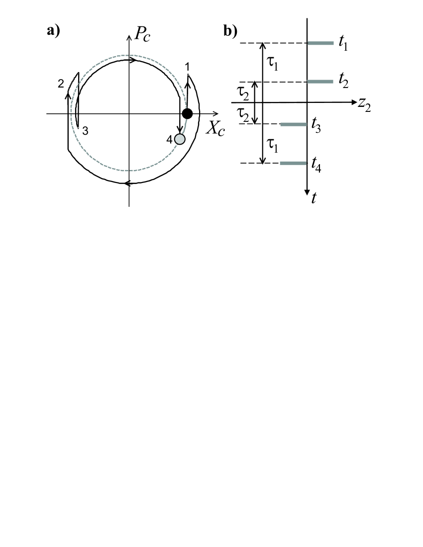
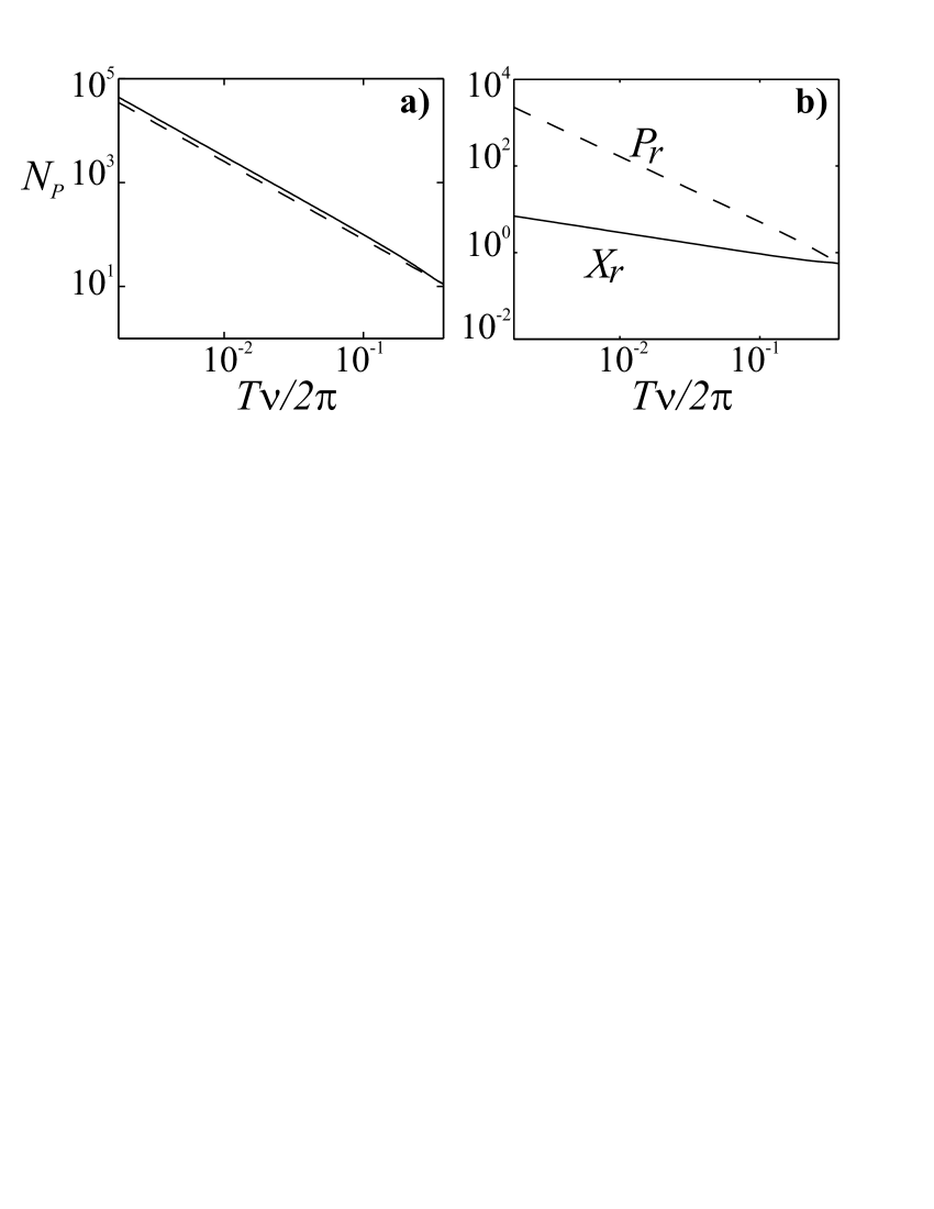
Figure 2: (a) Trajectory in phase space of the center-of-mass state of the ions $(\tilde{Q}_{c},\tilde{P}_{c})$ during the 2-qubit gate (solid line), connecting a possible initial state (black filled circle) to its final state (grey filled circle), for the protocol designed in Sec. III.2. Figure (b) shows how the laser pulses (bars) distribute in time for this scheme. Below we plot (c) the Number of pairs of pulses, and (b) relative angle of the two laser beams required to produce a phase gate using this scheme.

In Ref. García-Ripoll et al. (2003) we have found two possible solutions for these equations. The first protocol that we proposed, performs the phase gate in a time $T=1.08/\nu$, using about 4 pulses, while the second protocol allows for an arbitrarily short gating time $T\sim N_{p}^{-2/3}/\nu$ at the expense of using more pulses or kicks.

The method for the first protocol is illustrated in Fig. 2(a-b), where we plot the phase space trajectories followed by the center of mass mode. This sequence consists basically on four groups of pulses given by $(n_{l}/n,t_{l})=\{(\gamma,-\tau_{1}),(1,-\tau_{2}),(-1,\tau_{2}),(-\gamma,\tau_{1})\}$. The number $n$ tells us how many pulses are sent within each group, and the parameter $0<\gamma=\cos(\theta)<1.0$ is a real number that describes how much tilted are the kicking lasers with respect to the axis of the trap. It is always possible to find a solution to Eq. (26) with $\tau_{1}\simeq 0.538(4)(2\pi/\nu)>\tau_{2}>0$. The results for the performance of the gate are summarized in Fig. 2(c-d): for realistic values of the Lamb–Dicke parameter DeMarco et al. (2002) we only need to apply the sequence of pulses one or two times to implement a phase gate.

The second protocol performs the gate in an arbitrarily short time $T$. For shortening the time we now require six groups of pulses, distributed according to $(n_{l}/n,t_{n})=\{(-2,-\tau_{1}),(3,-\tau_{2}),(-2,-\tau_{3}),(2,\tau_{3}),(-3,\tau_{2}),(2,\tau_{1})\}$, where the times $\tau_{1}$, $\tau_{2}$ and $\tau_{3}$ are found numerically by solving the transcendental equations (26), with the constraint that the whole process takes a time $T=2\tau_{1}$. As Fig. 2 shows, the number of pulses, $N=14n$, increases with decreasing time as $N_{p}\propto T^{-3/2}$. This is just a consequence of a more general result that is shown later.

III.3 Phase gate based on continuous forces

The use of $\pi/2$ pulses to introduce momentum in the ions has some inconveniences. First of all, each of the pulses has to be perfect, and induce a complete population transfer from one internal state to the other one. If this is not the case, systematic errors on each of the pulses can lead to an exponential decrease of the fidelity. Furthermore, as we increase the gating speed, the pulses may become too long to be considered as instantaneous kicks, and the previous formalism fails.

What we have found, and what is also one of the main results of this paper, is that the phase gate may be produced also by applying continuous forces. The search for this forces is then no more difficult than solving an eigenvalue equation, where one may add restrictions such as smoothness of the force, and minimal total work.

Let us take the real vector space $L^{2}([0,T])$ of space of square integrable real forces in the $[0,T]$ interval, with the usual scalar product $(f,g)=\int_{0}^{t}f(t)g(t)dt$. From this Hilbert space, we choose a subspace ${\cal H}$ of functions which are orthogonal to the modes $e^{i\omega_{c,r}t}$

$$\int_{0}^{T}d\tau\,e^{i\omega_{c}\tau}F(\tau)=\int_{0}^{T}d\tau\,e^{i\omega_{r}\tau}F(\tau)=0.$$ (28)

Within ${\cal H}$, the phase and the smoothness of the gate are given by $\phi[F]=(F,{\cal G}F)$ and $S[F]:=(F,-\frac{d^{2}}{dt^{2}}F)$, respectively. We will prove that the optimal (i. e. smoothest) force that produces a phase gate $\phi=\pi/4$, is simply proportional to $F_{\mu}$, where $F_{\mu}$ is the eigenstate

$$-\mu\frac{d^{2}}{dt^{2}}F_{\mu}={\cal G}F_{\mu}$$ (29)

with largest eigenvalue $|\mu|$. If rather than measuring the optimality with $S[F]$ we use just the norm, $N[F]:=\|F\|_{2}=(F,F)$, then the eigenvalue problem is simpler

$$\mu F_{\mu}={\cal G}F_{\mu}.$$ (30)

Let us prove this useful result. We have to work with four functionals, which are the $S[F]$ and $\phi[F]$ defined above plus two more, which measure the displacements originated by the force: $D_{r,c}[F]=\int_{0}^{T}d\tau\,e^{i\omega_{c,r}\tau}F(\tau)$. By choosing the space of real periodic functions which are orthogonal to the Fourier modes $e^{i\omega_{c,r}\tau}$ we ensure that everything is well defined and also that the constraints $D_{c,r}[F]=0$ are satisfied. This leaves us with the problem of finding a force which minimizes $S[F]$, while satisfying the last constraint $\phi[F]=\pi/4$. There exists however a much easier dual problem which is formulated as finding the maximum of $\phi[F]$ subject to the quadratic constraint $S[F]=1$. Using the theory of Lagrange multipliers, this amounts to finding the maximum of

$${\cal L}[F]=\phi[F]-\mu(S[F]-1),$$ (31)

where $\mu$ is the Lagrange multiplier. Differentiating the Lagrangian we obtain Eq. (29), from where it follows that $\mu\|F\|_{2}^{2}=\phi$ is the maximal phase to be achieved, and the associated eigenstate $F_{\mu}\sqrt{\pi/(4\mu)}/\|F\|_{2}$ is the force we were looking for.

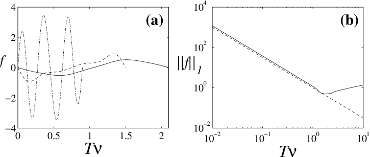
Figure 3: (a) Optimal forcing for a gating time $T\nu=2.1$ (solid), $1.5$ (dashed) and $0.9$ (dash-dot), where $\omega=2\pi\times\nu$ is the frequency of the ion trap. (b) Intensity of the force vs. duration of the gate (solid) and visual aid $(T\nu)^{-3/2}$ (dashed). All magnitudes have been adimensionalized following the text.

Even though we have been able to relate the control problem to an eigenvalue equation (29), there exists no simple analytical solution to this problem and we have to resort to some simple numerics. However, a very nice feature of the two-ion problem is that, by scaling quantities with respect to the trap strength, $\omega$, and the wavepacket size, $\alpha=(\hbar/m\omega)^{-1/2}$, we can compute the optimal force independent of the setup. Using these units and expanding the force in term of Fourier modes

$$f(t)=\sum_{m=-N_{m}}^{N_{m}}c_{n}e^{i2m\pi t/T}=\frac{F(t)\alpha}{\hbar\omega},$$ (32)

we can express Eq. (29) as an eigenvalue equation for the vector $\vec{c}$, that is to be solved numerically. The number of modes $N_{m}$ can in principle be any number above 3, because some degrees of freedom are lost when satisfying the constraint (16). However, the numerical experiments show that indeed $N_{m}=4$ provides very good solutions. As an example, in Fig. 3(a) we show three possible forces for a duration of the gate $T\omega/2\pi=2.1,1.5$ and $0.9$. We have computed other solutions for a wider range of gate speeds. In Fig. 3(b) we plot the mean intensity $\|f\|=\int_{0}^{T}|f(t)|dt$ versus the total time $T$, and demonstrate the law $T^{-3/2}$ obtained above.

An interesting question is how much energy we have to put into the system in order to produce faster and faster gates. With our current formalism, this can be answered very quickly. Let us assume that we have the optimal force that produces a phase gate in time $T\ll 2\pi/\omega_{c,r}$. Since the time is very short, we can perform a Taylor expansion of the function ${\cal G}(\tau)$ obtaining

$$|\phi| \simeq \left|\int_{0}^{T}\int_{0}^{T}d\tau_{1}d\tau_{2}F(\tau_{1})F(\tau_{2})\frac{(\omega_{c}^{2}-\omega_{r}^{2})}{12m\hbar}|\tau_{1}-\tau_{2}|^{3}\right|$$ (33)

$$\leq \frac{\omega_{c}^{2}-\omega_{r}^{2}}{12m\hbar}T^{3}\|F\|_{1}^{2}$$

where $\|F\|_{1}=\int_{0}^{T}d\tau\,|F(\tau)|$ is just a measure of the force applied. From here we see that

$$\|F\|_{1}\simeq T^{-3/2}$$ (34)

or, in the case of the kicked ions, $N_{p}\simeq T^{-3/2}$, the scaling that the numerical simulations already showed.

III.4 Adiabatic pushing

As a final remark, we want to relate the methods presented here with the pushing gate introduced in Ref. Cirac and Zoler (2000). That work proposed to trap the ions in separate microtraps, $V_{e,i}(x_{i})=\frac{1}{2}m\omega^{2}(x_{i}-x_{i}^{(0)})^{2}$, and to apply a state dependent force on two neighboring ions. This force should be switched on and off adiabatically with respect to the period of the traps, $2\pi/\omega$, in order to approach the ions to each other and later on return them to their equilibrium positions. The adiabaticity condition ensures that the ions remain at all times in the ground state of the effective Hamiltonian (4), which is now time dependent, because the equilibrium positions $x_{k}^{(0)}$ and the equilibrium energy $E_{0}$ both depend on the instantaneous value of the forces. After restoring the ions to their original positions, the only effect on the quantum state of the ions is a state-dependent phase

$$\phi=\int_{0}^{T}E_{0}\left[x_{1}^{(0)}(t),\ldots,x_{N}^{(0)}(t)\right]dt.$$ (35)

The previous analysis is found in Refs. Cirac and Zoler (2000); Calarco et al. (2001); Sasura and Steane (2003). A very important point is that, in order not to excite the ions and regard the process as truly adiabatic, the forces have to be weak and change very slowly, and no cubic contributions to the energy should appear. In other words, we should be able to describe the change of $E_{0}$ using at most quadratic terms, $E_{0}[\vec{x}^{(0)}(t)]\simeq E_{0}[\vec{x}^{(0)}(0)]+\frac{1}{2}mV_{ij}\delta x_{i}^{(0)}\delta x_{j}^{(0)}$. Hence, rather than using the adiabatic theorem we can integrate the problem exactly. For a single harmonic oscillator we get

$$z(t)=e^{-i\omega t}z_{0}+\frac{1}{\sqrt{2}}f(t)-\frac{1}{\sqrt{2}}\int_{0}^{t}d\tau\,e^{i\omega\tau}\frac{1}{\omega}f^{\prime}(\tau),$$ (36)

where the adiabatic condition corresponds to neglecting the last term $f^{\prime}(\tau)/\omega$, and the force only has to satisfy $f(T)=f(0)=0$. Repeating the arguments of previous sections, for two ions in neighboring traps the total phase becomes

$$\phi=\int_{0}^{T}d\tau\frac{\omega_{c}^{-1}-\omega_{r}^{-1}}{2m\hbar}F(\tau)^{2}\sigma^{z}_{1}\sigma^{z}_{2}.$$ (37)

Here $\omega_{c}=\omega$ and $\omega_{r}$ now depend slightly on the separation of the microtraps, but the same formula applies for the case in which both ions coexist in the same trap —a situation that could not be considered with the formalism of previous papers.

IV Quantum control of several ions

We will now study 1D setups with more than two ions. As we showed before, we can still control the geometric phases and use them to simulate a variety of spin Hamiltonians [Sec. IV.1]. The design of the forces for these simulations is still a control problem, but a much more difficult one. For instance, a crucial difference is that in setups with more than two ions either addressability or a spatial modulation of the forces are required. As a possible application of this result we study how to optimally generate entangled states and squeezing. In particular, we show that this can be done for a large number of ions (up to 30) in a very short time [Sec. IV.2].

IV.1 Simulation of spin Hamiltonians

Given any Ising Hamiltonian

$$H_{J}=\sum_{ij}J_{ij}\sigma^{z}_{i}\sigma^{z}_{j},\quad J=J^{t}\in\mathbb{R}^{N\times N},$$

and a time, $T$, it is possible to design a set of state dependent forces, $F_{i}(t;J)$ such that after applying these forces for a time $T$, the dynamics of the ions simulates this spin Hamiltonian. In other words

$${\cal T}\left[e^{i\int_{0}^{t}H(\tau)d\tau}\right]=e^{-iH_{J}T},$$

where ${\cal T}$ denotes time ordered product and $H$ is the true Hamiltonian of the ions (4).

The proof is very simple. Let us slice the time interval $[0,T]$ into $N^{2}$ subintervals, $0<t_{11}=t_{12}<\ldots<t_{N,N-1}<T$. In a given time interval, $I=[t_{ij},t_{i,j+1}]$, we will switch on two forces, and leave all other ions on their own,

$$F_{k}(t)=0,\;t\in[t_{ij},t_{i,j+1}],\;\forall k\neq i,j.$$

The active forces $F_{i}(t)$ and $F_{j}(t)$ must satisfy several equations

$$0=\int_{I}e^{i\omega_{k}\tau}M_{k\alpha}F_{\alpha}(\tau)d\tau,\;\alpha=i,j,\;k=1\ldots N$$ (38)

$$J_{ij}=\tfrac{1}{t_{i,j+1}-t_{ij}}\int_{I}\int_{I}d\tau_{1}d\tau_{2}\,F_{i}(\tau_{1}){\cal G}_{ij}(\tau_{1}-\tau_{2})F_{j}(\tau_{2}).$$

It is not difficult to convince oneself that these equations always have a solution, and that by repeating this procedure we will get an effective total phase, $\phi$, that resembles the one produced by the Ising model during a time $T$. $\square$

We have to make several remarks here. The first one is that since the operator that we want to simulate is symmetric, $J_{ij}=J_{ji}$, and since the diagonal terms only contribute to a global phase, the number of intervals can be actually decreased to $N(N-1)/2$.

However, more important is the fact that we can use coherent control to find optimal forces, $\vec{F}$, which instead of piecewise continuous are the smoothest possible and have the optimal norm, while giving rise to the same effective Hamiltonian. This task has been performed numerically for some models, and the results will be shown in the following section.

From the point of view of quantum simulation, we would like to be able to model more than just an Ising model, which is essentially classical. For instance, one would like to be able to introduce transverse magnetic fields, $\sum_{i}h_{i}\sigma^{x}_{i}$, or to simulate a Heisenberg interaction, $\vec{\sigma}_{i}\vec{\sigma}_{j}$, and in general, a unitary operation of the form (2) would be desirable. The answer to this problem is once more the stroboscopic evolution, or a Trotter expansion of the operator (2),

$$U\simeq\left\{\prod_{\alpha=x,y,z}e^{i\frac{T}{N}t\left(\sum_{ij}J^{\alpha}_{ij}\sigma^{\alpha}_{i}\sigma^{\alpha}_{j}+\sum_{i}h^{\alpha}_{i}\sigma^{\alpha}_{i}\right)}\right\}^{N}.$$ (39)

In this expansion, we decompose the total unitary as a product of phase gates, that are originated by forces that depend on $\sigma^{x}_{i}$, $\sigma^{y}_{i}$ and $\sigma^{z}_{i}$. In practice, one would switch on a magnetic field $h^{z}_{i}$ and perform a phase gate with coefficients $J^{z}_{ij}$ for a time $T/N$, rotate the spins so that $\sigma_{y}$ becomes $\sigma_{z}$, apply the phases with $J^{y}_{ij}$, etc.

It is also worth noticing that if we switch on the state-dependent forces acting on different ions, and make them oscillate with a single frequency $\Omega$ around a constant value, $F_{i}(t)=f_{i}\sin(\Omega t)\sigma^{z}_{i}$, for a long time, the effective interaction is a particular spin Hamiltonian

$$H=\sum_{ijk}f_{i}\frac{M_{ik}M_{jk}[1+\delta_{\Omega,0}]}{4m\hbar(\omega_{k}^{2}-\Omega^{2})}f_{j}\sigma^{z}_{i}\sigma^{z}_{j}+{\cal O}({f_{i}^{2}\over\omega_{k}^{2}}),$$ (40)

In the limit $\Omega\to 0$, this model corresponds to the one found in Porras and Cirac (2004). As it was shown there, depending on whether the forces operate longitudinally or transversely to the ion trap, this continuous force will give rise to long range or short range interactions.

IV.2 Coherent control and design of entanglers

The simulation of an Ising interaction is by itself interesting, and has important applications such as creation of many-qubit quantum gates, quantum simulation and adiabatic quantum computing. However, a most straightforward and useful application of an Ising Hamiltonian is the generation of many-body highly entangled states called graph states Hein et al. (2004). Roughly speaking, let us imagine that we have a set of $N$ spins, which we represent by points or vertices, and let us connect these points by lines or edges. The resulting graph can be described by an adjacency matrix which takes value $J_{ij}=1$ only if the spins $i$ and $j$ are connected. To each graph we can thus associate a Hamiltonian of the form $H_{J}=\sum_{i,j}J_{ij}\sigma^{z}_{i}\sigma^{z}_{j}$. It has been shown that after applying this interaction over a certain time on a transversely polarized state, the outcome is a highly entangled state called a graph state:

$$\left|\psi_{G}\right\rangle=\frac{1}{2^{N/2}}e^{-i\frac{\pi}{8}H_{\cal G}}\left(\left|0\right\rangle+\left|1\right\rangle\right)^{\otimes N}.$$ (41)

When the graph has a lattice geometry, these states are also known as cluster states Briegel and Raussendorf (2001), and form the basic ingredient of the one-way quantum computer Raussendorf and Briegel (2001). However, a particularly important case without lattice geometry is the GHZ state,

$$\left|\mathrm{GHZ}\right\rangle\sim\left|0\right\rangle^{\otimes N}+\left|1\right\rangle^{\otimes N},$$ (42)

which is essentially generated by the interaction $J_{ij}=1$ or $H_{J}=(\sum_{i}\sigma^{z}_{i})^{2}$. The GHZ state is one of the best studied entangled states, it constitutes a canonical example of Schrödinger cat state, and it could have important applications in the field of precision frequency measurements, providing a $1/\sqrt{N}$ precision increase for $N$ entangled ions Wineland et al. (1992, 1994), a point already demonstrated experimentally in Ref. Meyer et al. (2001).

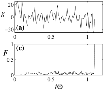
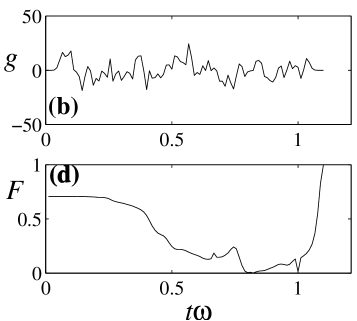
Figure 4: Generation of a (a,c) cluster state of $N=10$ ions and of (b,d) a GHZ state of $N=20$ ions, using common forcing for a time $T=1.1/\omega$. (a,c) Time dependence of the forces, $f(t)$. (b,d) Fidelity with respect to the target state as a function of time.

We have investigated how to implement these highly entangled states using our quantum control techniques. The idea is very simple: we design a matrix $J_{ij}$ for our graph state, and look for the time- and state-dependent forces that implement the phase transformation $\exp(-i\pi H_{J}\pi/4)$ within a fixed time $T$. For simplicity, even though it is not warranted to succeed, we look for forces that have a common time dependence $F_{i}(t)=\gamma_{i}f(t)\sigma^{z}_{i}$, $|\gamma_{i}|\leq 1$. These forces could be implemented with an appropriate intensity mask, which determines the relative amplitudes $\gamma_{i}$, and a global intensity modulation, which gives the function $f(t)$. Expanding this modulation in Fourier modes, we find $N(N-1)/2+N$ equations which define a possible entangling procedure. We have solved numerically these equations, both for the GHZ state and for the cluster state. While in the first case we always found exact solutions with a small number of modes (i.e. $50$ modes for $30$ ions), the generation of the cluster state was always approximate with high fidelity, $F\simeq 99.9\%$. The error in this case has its origin in our particular choice of forces.

In Fig. 4 we show the entangling procedure for a setup with $10$ and $20$ ions, even though chains of up to $30$ ions have been considered. We measure the fidelity of the process as the overlap between the target state and the one achieved. If $\delta J$ is the difference between the desired interaction and the achieved one, then $F=\frac{1}{2^{N}}\sum_{\vec{s}}e^{-i\vec{s}^{t}\delta JT\vec{s}}$, where the sum is performed over all possible spin configurations, $s_{k}=\pm 1$. The time scales for the generation of the interaction are independent of the size of the system, and for instance we can produce a GHZ state of $20$ ions in a time $T=1.1/\omega$, to be compared with the time $T=3000\pi/\omega$ required when individually addressing one of the vibrational modes Mølmer and Sørensen (1999). The strength of the forces, though, grows moderately with the number of ions, which can be inconvenient. However, thanks to the periodicity of the forcing, $f(t)$, if we divide the intensity of the forces by a factor of 2, $f(t)\to f(t)/2$, the same gate be produced in a longer time $4T$. Furthermore, the forces that we present in this paper are not optimal, and have been found with a straightforward Gauss-Newton method. If high fidelity is not required, one may find better solutions with fewer modes, but most important we expect significant improvements by the application of better numerical algorithms to search for the optimal entanglers.

Using the Ising interaction we can not only produce graph states, but also squeezed states: states in which the variance of one spin component, $\Delta S_{x}$, has been decreased at the expense of increasing the other variances. As it was shown in Kitagawa and Ueda (1993), a Hamiltonian of the form $H=J_{z}^{2}$ (single axis squeezing) or $H=J_{x}^{2}-J_{y}^{2}$ (two-axis squeezing) can be used to produced squeezing. Both models can be simulated using our tools, either directly, as in the single-axis squeezing, or stroboscopically, for the XY interaction. Indeed, the stroboscopic simulation of the two-axis squeezing resembles the scheme of $\pi/2$ pulses used in Jaksch et al. (2002) to effectively switch off the interaction in two-mode Bose-Einstein condensates Sorensen et al. (2001).

V Optimal control of errors

Up to now, we have assumed that the motion of the ions is not disturbed during the time when the controlling forces are applied. In this section we will show how to take these effects into account for a realistic model of dissipation. The main result is that the fidelity of the process can still be computed and that the there are two sources of error: one due an imperfect control of the ions, which introduces some temperature dependence on the fidelity [Sec. V.3], and another one due to the dissipation, that can be treated as another constraint for the control problem [Sec. V.2]. Finally, we will comment on possible extensions outside the harmonic regime [Sec. V.4]

V.1 The model and a exact solution

We study the dissipation with a master equation that arises from coupling the phonon modes with a “classical” bosonic bath in thermal equilibrium

$$\frac{d}{dt}\rho = \frac{i}{\hbar}[H_{I},\rho]+\sum_{k}\gamma N_{k}(2a_{k}^{\dagger}\rho a_{k}-a_{k}a_{k}^{\dagger}\rho-\rho a_{k}a_{k}^{\dagger})$$ (43)

$$+ \sum_{k}\gamma_{k}(N_{k}+1)(2a_{k}\rho a_{k}^{\dagger}-a_{k}^{\dagger}a_{k}\rho-\rho a_{k}^{\dagger}a_{k}).$$

Here $\gamma_{k}$ describes the coupling to an external bath and $N_{k}$ is the mean number of bosons on that bath and it is related to its temperature. The Hamiltonian in Eq. (43) is written in the interaction picture

$$H_{I}=\sum_{ki}\hbar(g_{ki}(t)a_{k}+g_{ki}^{\star}a_{k}^{\dagger})\sigma^{z}_{i}.$$ (44)

In order not to obscure the discussion, we will assume that each phonon mode interacts with an independent bath. In that case, the forces in the rotating frame of reference become, $\hbar g_{ki}(t)=\tfrac{1}{\sqrt{2}}F_{i}(t)M_{ik}\alpha_{k}e^{-i\omega_{k}t}$. However, it is easy to generalize the following analysis to a more realistic model in which each ion couples independently to the environment, and the operators $a_{k}$ and $a_{k}^{\dagger}$ do not represent the phonons, but the displacements of the ions.

To study the fidelity of a gate we only need to know the matrix elements of the reduced density matrix for the internal degrees of freedom. This matrix may be written as a collection of expectation values,

$$\rho_{real}=\sum_{\mathbf{s},\mathbf{r}}\langle\Sigma_{\mathbf{s,r}}\rangle\Sigma_{\mathbf{s,r}},$$ (45)

where $\Sigma_{\mathbf{s,r}}=|s_{1}\ldots s_{N}\rangle\langle r_{1}\ldots r_{N}|$, $r_{k},s_{k}=\pm 1$ form a complete basis for the space of $2^{N}\times 2^{N}$ complex matrices.

The calculations that provide us with the evolution of $\langle\Sigma_{\mathbf{s,r}}\rangle$ are detailed in Appendix A. Here we will only summarize the main result, which is that the reduced density matrix can be written as

$$\langle\Sigma_{\mathbf{s},\mathbf{r}}\rangle(t)=e^{-\kappa_{\mathbf{s},\mathbf{r}}}e^{-i\sum_{jk}J_{jk}s_{j}s_{k}}\langle\Sigma_{\mathbf{s},\mathbf{r}}\rangle(0)e^{i\sum_{jk}J_{jk}r_{j}r_{k}}.$$ (46)

In other words, the spin density matrix has the form

$$\rho_{real}(t)=e^{-{\cal L}}\left[U\rho_{real}(0)U^{\dagger}\right],$$ (47)

where $U=\exp(-i\sum J_{jk}\sigma^{z}_{j}\sigma^{z}_{k})$ is the operation that we want to perform, and ${\cal L}(\rho)=\sum_{\mathbf{s},\mathbf{r}}\kappa_{\mathbf{s,r}}\Sigma_{\mathbf{s,r}}\rho\Sigma_{\mathbf{s,r}}$ is responsible for the decay of coherences.

In comparison with the previous part of the paper, the unperturbed orbits in phase space, that is the evolution without external forcing, are now not circular orbits, but by spirally decaying ones. This fact translates in the new conditions for uncoupling internal and motional degrees of freedom (20)

$$\int_{0}^{t}d\tau e^{-(i\omega_{k}+\gamma_{k})\tau}F_{j}(\tau)=0,\;\forall\,j,k$$ (48)

which now depend on the exponential decay rate, $\gamma_{k}$, given by our dissipation model. This model-dependence is also evident in the kernel that produces our unitary operation, $J_{ij}$, which now reads

$${\cal G}_{jl}(\tau)=\sum_{k}\frac{M_{jk}M_{lk}\alpha_{k}^{2}}{2m\omega_{k}\hbar}\sin(\omega_{k}|\tau|)e^{\gamma_{k}|\tau|}.$$ (49)

Finally, we would like to remark that the conditions, the phase and the kernel are only slightly modified when we consider a local coupling to the environment.

V.2 Quantum control of errors due to dissipation

To understand better the implications of Eq. (47), let us study the dynamics of a single ion. In this case the reduced density matrix can be expressed uniquely in terms of the expectation values $\langle\sigma^{z}\rangle$ and $\langle\sigma^{+}\rangle$. Furthermore, since the magnetization is constant, we can compute the Uhlmann fidelity exactly as a function of $\langle\sigma^{+}\rangle$. Let us assume that initially the system is in a pure state, and define $\langle\sigma^{+}\rangle_{real}=e^{i\delta\phi-\kappa}\langle\sigma^{+}\rangle_{id}$, where the subindex “id” denotes the ideal value obtained in absence of errors. The Uhlmann fidelity of the gate is Nielsen and Chuang (2000)

$${\cal F}(\rho_{real},\rho_{id})=\sqrt{1+|\langle\sigma^{+}\rangle_{id}|^{2}(2e^{-\kappa}\cos(\delta\phi)-1)}.$$ (50)

Two types of errors contribute to the decay of the fidelity. The first type is made of control errors. These errors contribute both to the spurious phases ($\delta\phi$) and to an effective decay due to not restoring the motional state of the ions ($\kappa\neq 0$ because $\beta(T)\neq 0$ and $U(T)\neq 1$). These errors cause a smooth dependence on the temperature to appear, as shown later in Sec. V.3.

The second type of errors are due to dissipation during the forcing of the ions. Their contribution to the exponential decay is

$$\kappa_{\text{dissip}}=\gamma(N+\tfrac{1}{2})\int_{0}^{t}d\tau|\beta(\tau)|^{2}.$$ (51)

One would be led to think that if dissipation acts on a much larger scale than the time required to perform our gate we can neglect it completely. However, a simple argument shows that this is not the case. As we saw before in Sec. III.3, the strength of the forces scales roughly as $F\simeq T^{-5}$. This scaling allows us to give a worst case estimate of $\beta(t)\simeq Ft$ and conclude

$$\kappa_{\text{dissip}}\sim\gamma T^{-2},\quad T\ll 1/\omega.$$ (52)

What this means is that slower gates will involve smaller displacements of the ions, which in turn translates into less dissipation. On the other hand, a too long application of a force also gives more time for the dissipation to operate and the optimal duration should be a compromise between both processes. It is thus possible and recommended to optimize the forces $F(t)$ taking not only into account the properties of the force (i.e. differentiablity and intensity), but also trying to minimize the decay $\kappa$ induced by the force. From the numerical point of view, this new control problem is only slightly more complicated than the ones we have solved in Secs.  III-IV, because $\kappa_{\text{dissip}}$ is a nonlinear function of the forces.

V.3 Errors due to an imperfect control: influence of temperature

Let us denote by $U_{id}=\exp(\sum_{ij}J_{ij}\sigma^{z}_{i}\sigma^{z}_{j})$ the ideal operation that we want to perform, and by $U_{real}$ the operation with errors. In this section, the only source of error that we consider is an imperfect control, denoted by a perturbation of the state-dependent force induced on the ions, $(F_{i}(t)+\delta F_{i}(t))\sigma^{z}_{i}$. According to the previous analysis, the effect of this perturbation will be a residual state-dependent displacement of the coherent wavepackets at the end of the process, $\beta_{k}(T)$,

$$\beta_{k}=-i\int_{0}^{T}d\tau\,e^{i\omega_{k}\tau}\frac{\alpha_{k}M_{ik}\delta F_{i}(t)}{\hbar\sqrt{2}}\sigma^{z}_{i}=:\sum_{k,i}\beta_{ki}\sigma^{z}_{i}.$$ (53)

plus a perturbation of the phase

$$\delta\phi=\sum_{ij}\delta J_{ij}\sigma^{z}_{i}\sigma^{z}_{j},$$ (54)

which can be interpreted as a change in the effective interaction between ions [Sec. IV]

$$\delta J_{ij} = \int_{0}^{T}\int_{0}^{T}d\tau_{1}d\tau_{2}\,{\cal G}_{ij}(\tau_{2}-\tau_{1})\times$$

$$\times[F_{i}(\tau_{1})\delta F_{j}(\tau_{2})+\delta F_{i}(\tau_{1})F_{j}(\tau_{2})].$$

We will assume as initial condition a pure state of the internal degrees of freedom and a thermal state of the vibrational ones $\rho(0)=|\psi\rangle\langle\psi|\otimes\rho_{vib}(T)$. The Uhlmann fidelity at the end of the process is given by

$${\cal F}(\rho_{id},\rho_{real}(t)) = \mathrm{Tr}_{vib}(\langle\psi|U_{id}^{\dagger}\rho(t)U_{id}|\psi\rangle)$$ (55)

$$= \langle\psi|\mathrm{Tr}_{vib}[U_{id}^{\dagger}\rho(t)U_{id}]|\psi\rangle.$$

Expanding $|\psi\rangle=\sum c_{\mathbf{s}}|s_{1}\ldots s_{N}\rangle$, we obtain

$${\cal F}=\sum_{\mathbf{s},\mathbf{r}}c_{\mathbf{s}}^{\star}c_{\mathbf{r}}\langle\Sigma_{\mathbf{s},\mathbf{r}}\rangle_{\rho(t)}.$$ (56)

When we neglect dissipation, the previous expectation values can be computed in terms of the final displacements, $\beta_{k}(t)$, and the residual phases as follows:

$$\langle\Sigma_{\mathbf{s},\mathbf{r}}\rangle_{U_{id}^{\dagger}\rho(t)U_{id}}=\mathrm{Tr}\left\{\prod_{k}D[\beta_{k}(t)(s_{k}-r_{k})]\rho_{vib}(T)\right\}\times$$ (57)

$$\times e^{i(\mathbf{s}^{t}\delta J\mathbf{s}-\mathbf{r}^{t}\delta J\mathbf{r})}c_{\mathbf{s}}c_{\mathbf{r}}^{\star}$$

Here $D(z)=\exp(za^{\dagger}-z^{\star}a)$ is the displacement operator, $\rho_{vib}(T)$ is a thermal state

$$\rho_{vib}(T)=\bigotimes_{k=1}^{N}\frac{\hbar\omega_{k}}{\pi k_{B}T}\iint dzd\bar{z}\,e^{-|z|^{2}\hbar\omega_{k}/k_{B}T}|z\rangle_{k}\langle z|,$$ (58)

and thus $\langle D(z)\rangle=\exp[-|z|^{2}(1/2+k_{B}T/\hbar\omega_{k})]\equiv\exp(C_{k})$ so that the total fidelity becomes

$${\cal F}=\sum_{\mathbf{s},\mathbf{r}}|c_{\mathbf{s}}|^{2}||c_{\mathbf{r}}|^{2}e^{i(\mathbf{s}^{t}\delta J\mathbf{s}-\mathbf{r}^{t}\delta J\mathbf{r})}e^{C_{k}(s_{k}-r_{k})^{2}}.$$ (59)

V.4 Errors due to larger displacements

The previous studies can be generalized to arbitrary interactions and trapping potentials. Let us assume a complicated Hamiltonian

$$H=\sum_{i}\left[\frac{p_{i}^{2}}{2m}-f_{i}(t)\sigma^{z}_{i}x_{i}\right]+V(x_{1},\ldots,x_{N}),$$ (60)

describing the traps and the ion-ion interaction. The evolution equation for the position of the ions are of the form

$$\dot{x}_{i}=\frac{p_{k}}{m},\;\dot{p}_{i}=-\frac{\partial V}{\partial x_{i}}+f_{i}(t)\sigma^{z}_{i}.$$ (61)

Since the operators $\sigma^{z}_{i}$ are conserved quantities, the previous equations can be thought of as a simple problem of Newtonian mechanics, even though in practice, both $x_{i}$ and $p_{i}$ are operators. We can thus represent a general solution as $\{x_{i}(t;\sigma),p_{i}(t;\sigma)\}$, where $\sigma$ denotes the values of $\sigma^{z}_{i}$ operators. The phase of the ions is then computed by analyzing the evolution of the $\sigma^{+}_{i}$ operators. These operators must undergo a unitary transformation $\sigma^{+}(t)=U(t)\sigma^{+}_{i}(0)U^{\dagger}(t)$ in which the dependence on the $\{\sigma_{i}^{z}\}$ operators must be of the form

$$U(t)=\exp[\sum_{i}\theta_{i}(t)\sigma^{z}_{i}+\sum_{ij}\phi_{ij}(t)\sigma^{z}_{i}\sigma^{z}_{j}]=e^{i\phi}.$$ (62)

Using the commutation relation $[\sigma^{+}_{i},\sigma^{z}_{j}]=-2\delta_{ij}\sigma^{z}_{i}\sigma^{+}_{i}$, we obtain

$$\sigma_{i}^{+}(t)=e^{2\theta_{i}\sigma^{z}_{i}+2\sum_{j\neq i}\phi_{ij}(t)\sigma^{z}_{i}\sigma^{z}_{j}}\sigma_{i}^{+}(0).$$ (63)

Combining this with the Heisenberg equation for $\sigma_{i}^{+}$

$$i\hbar\frac{d\sigma^{+}_{i}}{dt}=2f_{i}(t)x_{i}\sigma^{z}_{i}\sigma^{+}_{i}=2\frac{\partial^{2}\phi}{\partial t\partial\sigma^{z}_{i}}\sigma^{+}_{i},$$ (64)

we find, up to global phases,

$$\phi\sim\sum_{i}\int_{0}^{T}d\tau f_{i}(\tau)x_{i}(\tau)\sigma^{z}_{i}.$$ (65)

From this analysis we see that we must impose two conditions on the process. On one hand, the orbits of the ions must be periodic so as to disentangle the internal and motional degrees of freedom

$$x_{i}(T;\sigma)\simeq x_{i}(0),\;p_{i}(T;\sigma)\simeq p_{i}(0).$$ (66)

On the other hand, the phase $\phi$ must be independent of the initial conditions, $\{x_{i}(0),p_{i}(0)\}$. Satisfying both conditions is impossible in general, but if we restrict ourselves to small displacements and harmonic restoring forces, $\partial V/\partial x_{i}\simeq\sum_{j}V_{ij}x_{j}$, it is possible to integrate Eq. (61) and recover our expressions for the phases (18).

If, however, the qubit and higher terms in $V(x_{1},\ldots,x_{N})$ become important, we will fail the restoring condition (66), and induce some entanglement between the motion and the spin of the ions. The errors due to these anharmonic terms are of the order

$$\left|\frac{\partial^{3}V}{\partial x_{i}\partial x_{j}\partial x_{l}}x_{i}x_{j}x_{l}\right|\sim\frac{3\hbar\omega\alpha}{d}\left|\frac{x}{\alpha}\right|^{3},$$ (67)

where $\alpha\simeq\sqrt{\hbar/m\omega}$ is the length associated to the harmonic oscillator, $d^{3}=e^{2}/2\pi\epsilon_{0}m\omega^{2}$ is the equilibrium distance between two ions, and $x$ is a typical displacement. Since a trivial analysis of these errors is not possible, we can only produce a pessimistic, first order bound that restricts the error induced by this perturbation on the wavefunction. First we will give a worst case prediction for the maximum displacement of the ions as $x_{max}<F_{max}T^{2}/2m$, where $F_{max}$ is the maximal force applied on the ions. Next we will use the scaling $\phi\sim\omega^{2}T^{5}F_{max}/\hbar m$ to show that roughly $(x_{max}/\alpha)\sim\phi/4\omega T$. With this, and first order perturbation theory we compute the error and estimate it as

$$E_{anh}=\left(\frac{\alpha}{d}\right)^{2}\frac{\phi^{3/2}}{4^{3/2}\omega T}.$$ (68)

If we want to apply our phase operations to build a quantum computer, we need $E<10^{-4}$ and there is a limit on the speed of the gate $T>10^{-3}/\omega$, which nevertheless gives gating rates of the order of 100 MHz.

VI Conclusions

We have developed a unified framework to study the coherent control of trapped ions by means of state-dependent forces and robust geometric phases. Our techniques can be used to perform fast two-qubit gates between pairs of ions. For an adiabatic switching of the forces and for the case of pulsed lasers we are able to reproduce the proposals of Cirac and Zoler (2000) and García-Ripoll et al. (2003), and with very little work we can design the optimal forces that produce a phase gate in a given time with the lowest intensity. Using the same tools and a larger number of ions, we can simulate either continuously or stroboscopically a number of spin $s=1/2$ Hamiltonians. Furthermore, we are also able to create highly entangled states and squeezing, and as prototypical examples we have shown how to obtain a $GHZ$ state of $20$ ions in a very short time, $T=1.1/\omega$. Finally we have studied the sources of error in the application of our gate, which are an imperfect control, dissipation and anharmonic terms in the interaction. The first type of errors could be ideally corrected and introduce a smooth decay of the fidelity with the temperature. The second type of errors induces also a decay of the fidelity, but the amount of this error can be optimized using the tools of quantum control. Both dissipation and anharmonicity set up upper limits on the speed of the gate. This limit is however very weak, since it allows theoretically a gating speed of hundreds of MHz, and it could be overcome by a numerical study of the role of anharmonic terms in the motion of the ions.

While concluding this paper we became aware of the work by P. Staanum, M. Drewsen and K. Mølmer Staanum et al. (2004) on performing quantum gates using continuous laser beams. The ideas shown in Ref. Staanum et al. (2004) are equivalent to the development of a two-qubit gate done in Sect. , with the difference that we provide an optimal solution for the problem.

J.J.G.-R. thanks J. Pachos, D. Porras and Shi-Liang Zhu for interesting discussions during the development of this manuscript. Part of this work was supported by the EU IST project RESQ, the EU project TOPQIP, the DFG (Schwerpunktprogramm Quanteninformationsverarbeitung) and the Kompetenznetzwerk Quanteninformationsverarbeitung der Bayerischen Staatsregierung. Research at the University of Innsbruck is supported by the Austrian Science Foundation, EU Networks and the Institute for Quantum Information.

Appendix A Solution of the master equation

As we mentioned before, the density matrix is characterized by the expectation values $\langle\Sigma_{\mathbf{s,r}}\rangle$. However, it is much more difficult to work with these expectation values, than with

$$A:=\Sigma_{\mathbf{s,r}}V(t):=\Sigma_{\mathbf{s,r}}e^{\sum_{k}(\beta_{k}a_{k}^{\dagger}-\beta^{\star}_{k}a_{k})}.$$ (69)

By imposing that $V(0)=1$ and that $V(T)$ is at most a phase, we will be able to relate the reduced density matrices $\rho_{real}(0)$ and $\rho_{real}(T)$. It is easy to see that indeed the operator $V(t)$ is a displacement operator and that Eq. (69) is essentially the solution of the nondissipative case, where $\beta_{k}$ measures the separation in phase space between configurations with internal states $\mathbf{s}$ and $\mathbf{r}$.

The equation for the expectation value of an arbitrary operator, $A$, can be written as follows

$$\frac{d}{dt}\langle{A}\rangle = \langle\partial_{t}A\rangle+\tfrac{i}{\hbar}\langle[H_{I},A]\rangle-\gamma\langle(D_{a}A)a+a^{\dagger}(D_{a})\rangle$$ (70)

$$+ \gamma N\langle D_{a}D_{a^{\dagger}}A+D_{a^{\dagger}}D_{a}A\rangle.$$

Here, $D_{a}A:=[A,a^{\dagger}]$ and $D_{a^{\dagger}}A:=[a,A]$ are two superoperators which first of all commute, $[D_{a},D_{a^{\dagger}}]=0$, and second they are related to the formal derivatives with respect to the operators $a$ and $a^{\dagger}$. So, for instance, $D_{a}f(a,a^{\dagger})=\partial_{a}f(a,a^{\dagger})$ for any analytical function $f$.

If we substitute Eq. (69) into Eq. (70), and use

$$\partial_{t}A = \sum_{k}\frac{\partial A}{\partial\beta_{k}}\dot{\beta}_{k}+\sum_{k}\frac{\partial A}{\partial\beta_{k}^{\star}}\dot{\beta}_{k}^{\star}$$ (71)

$$= U\left[\dot{\beta}_{k}(a^{\dagger}_{k}-\tfrac{1}{2}\beta^{\star}_{k})+\dot{\beta}_{k}^{\star}(-a_{k}-\tfrac{1}{2}\beta_{k})\right],$$

we will obtain

$$\frac{d}{dt}\langle A\rangle = i\sum_{k}\left\langle A\left[(g_{k\mathbf{r}}-g_{k\mathbf{s}})a_{k}+g_{k\mathbf{r}}\beta_{k}+\mathrm{H.~{}c.}\right]\right\rangle$$ (72)

$$+ \sum_{k}\left\langle A\left[\dot{\beta}_{k}a^{\dagger}_{k}-\dot{\beta}^{\star}_{k}a_{k}+\tfrac{1}{2}(\dot{\beta}_{k}\beta^{\star}_{k}-\beta_{k}\dot{\beta}_{k}^{\star})\right]\right\rangle$$

$$+ \sum_{k}\gamma_{k}N_{k}\left\langle A(-\beta_{k}^{\star}a_{k}+\beta_{k}a_{k}^{\dagger})\right\rangle$$

$$- \sum_{k}\gamma_{k}\left(N_{k}+\tfrac{1}{2}\right)|\beta_{k}|^{2}\langle A\rangle,$$

whith the new parameters $g_{k\mathbf{r}}:=\sum_{i}g_{ki}(t)r_{i}$.

Here is where we impose a particular evolution of the displacements on phase space, $\dot{\beta}_{k}+\gamma_{k}\beta_{k}+i(g_{k\mathbf{r}}^{\star}-g_{k\mathbf{s}}^{\star})=0$. This equation has a trivial solution

$$\beta_{k}(t)=i\int_{0}^{t}d\tau\,e^{-\gamma_{k}(t-\tau)}[g_{k\mathbf{r}}^{\star}(\tau)-g_{k\mathbf{s}}^{\star}(\tau)].$$ (73)

After substituting this value all terms containing Fock operators are cancelled and we are left with

$$\frac{d}{dt}\langle A\rangle=(-\dot{\kappa}+i\dot{\phi})\langle A\rangle,$$ (74)

where the decay $\kappa$ is

$$\kappa(t)=\sum_{k}\gamma_{k}\left(N_{k}+\tfrac{1}{2}\right)\int_{0}^{t}d\tau\,|\beta_{k}(\tau)|^{2},$$ (75)

and the total phase $\phi=\sum_{ij}J_{ij}(r_{i}+s_{i})(r_{j}-s_{j})$ is determined by the matrix

$$J_{ij}:=\mathrm{Im}\int_{0}^{t}d\tau_{1}\int_{0}^{\tau_{1}}d\tau_{2}\,g_{ki}(\tau_{1})g_{kj}(\tau_{2})^{\star}e^{-\gamma_{k}(\tau_{2}-\tau_{1})},$$ (76)

Using the symmetry of this matrix, the formula for the phase can be rewritten as $\phi=\sum_{ij}J_{ij}(r_{i}r_{j}-s_{i}s_{j})$, and the results mentioned in Sect. V.1 quickly follow.

References

- Cirac and Zoler (2000) J. I. Cirac and P. Zoler, Nature 404, 579 (2000).
- García-Ripoll et al. (2003) J. J. García-Ripoll, P. Zoller, and J. I. Cirac, Phys. Rev. Lett. 91, 157901 (2003).
- Levi (2003) B. G. Levi, Phys. Today 56, 17 (2003).
- Monroe et al. (1995) C. Monroe, D. M. Meekhof, B. E. King, W. M. Itano, and D. J. Wineland, Phys. Rev. Lett. 75, 4714 (1995).
- DeMarco et al. (2002) B. DeMarco, A. Ben-KIsh, D. Leibfried, V. Meyer, M. Rowe, B. M. Jelenkovic, W. M. Itano, J. Briton, C. Langer, T. Rosenband, et al., Phys. Rev. Lett. 89, 267901 (2002).
- Leibfried et al. (2003) D. Leibfried, B. DeMarco, V. Meyer, D. Lucas, M. Barret, J. Britton, W. M. Itano, B. Jelenkovic, C. Langer, T. Rosenband, et al., Nature 422, 412 (2003).
- Schmidt-Kaler et al. (2003) F. Schmidt-Kaler, H. Häffner, M. Riebe, S. Gulde, G. P. T. Lancaster, T. Deuschle, C. Becher, C. F. Roos, J. Eschner, and R. Blatt, Nature 422, 408 (2003).
- Kielpinski et al. (2002) D. Kielpinski, C. Monroe, and D. J. Wineland, Nature 417 (2002).
- Rowe et al. (2002) M. A. Rowe, A. Ben-Kish, B. DeMarco, D. Leibfried, V. Meyer, J. Beall, J. Britton, J. Hughes, W. M. Itano, B. Jelenkovic, et al., Quantum Inf. and Comput. 2, 257 (2002).
- Wineland et al. (1992) D. J. Wineland, J. J. Bollinger, W. M. Itano, F. L. Moore, and D. J. Heinzen, Phys. Rev. A 46, R6797 (1992).
- Wineland et al. (1994) D. J. Wineland, J. J. Bollinger, W. M. Itano, and D. J. Heinzen, Phys. Rev. A 50, 67 (1994).
- Steinbach and Gerry (1998) J. Steinbach and C. C. Gerry, Phys. Rev. Lett. 81, 5528 (1998).
- Mølmer and Sørensen (1999) K. Mølmer and A. Sørensen, Phys. Rev. Lett. 82, 1835 (1999).
- Sørensen and Mølmer (2000) A. Sørensen and K. Mølmer, Phys. Rev. A 62, 022311 (2000).
- Unanyan and Fleischhauer (2003) R. G. Unanyan and M. Fleischhauer, Phys. Rev. Lett. 90, 133601 (2003).
- Turchette et al. (1998) Q. A. Turchette, C. S. Wood, B. E. King, C. J. Myatt, D. Leibfried, W. M. Itano, C. Monroe, and D. J. Wineland, Phys. Rev. Lett. 81, 3631 (1998).
- Sackett et al. (2000) C. A. Sackett, D. Kielpinski, B. E. King, C. Langer, V. Meyer, C. J. Myatt, M. Rowe, Q. A. Turchette, W. M. Itano, D. J. Wineland, et al., Nature 404, 256 (2000).
- Meyer et al. (2001) V. Meyer, M. A. Rowe, D. Kielpinski, C. A. Sackett, W. M. Itano, C. Monroe, and D. J. Wineland, Phys. Rev. Lett. 86, 5870 (2001).
- Porras and Cirac (2004) D. Porras and J. I. Cirac, Phys. Rev. Lett. 92, 207901 (2004).
- (20) J. Barjaktarevic, G. J. Milburn, and R. H. McKenzie, arXive:quant-ph/0401137.
- Cirac and Zoller (1995) J. I. Cirac and P. Zoller, Phys. Rev. Lett. 74, 4091 (1995).
- Poyatos et al. (1998) J. F. Poyatos, J. I. Cirac, and P. Zoller, Phys. Rev. Lett. 81, 1322 (1998).
- Sørensen and Mølmer (1999) A. Sørensen and K. Mølmer, Phys. Rev. Lett. 82, 1971 (1999).
- Jonathan et al. (2000) D. Jonathan, M. B. Plenio, and P. L. Knight, Phys. Rev. A 62, 042307 (2000).
- James (2000) D. F. V. James, Fortschr. Phys. 48, 9 (2000).
- Milburn et al. (2000) G. J. Milburn, S. Schneider, and D. F. V. James, Fortschr. Phys. 48, 9 (2000).
- (27) L.-M. Duan, arXiv:quant-ph/041185.
- Staanum et al. (2004) P. Staanum, M. Drewsen, and K. Mølmer, Phys. Rev. A 70, 052327 (2004).
- Aharonov and Anandan (1987) Y. Aharonov and J. Anandan, Phys. Rev. Lett. 58, 1593 (1987).
- Calarco et al. (2001) T. Calarco, J. I. Cirac, and P. Zoller, Phys. Rev. A 63, 062304 (2001).
- Sasura and Steane (2003) M. Sasura and A. M. Steane, Phys. Rev. A 67, 062318 (2003).
- Hein et al. (2004) M. Hein, J. Eisert, and H. J. Briegel, Phys. Rev. Lett. 69, 062311 (2004).
- Briegel and Raussendorf (2001) H. J. Briegel and R. Raussendorf, Phys. Rev. Lett. 86, 910 (2001).
- Raussendorf and Briegel (2001) R. Raussendorf and H. J. Briegel, Phys. Rev. Lett. 86, 5188 (2001).
- Kitagawa and Ueda (1993) M. Kitagawa and M. Ueda, Phys. Rev. A 47, 5138 (1993).
- Jaksch et al. (2002) D. Jaksch, J. I. Cirac, and P. Zoller, Phys. Rev. A 65, 033625 (2002).
- Sorensen et al. (2001) A. Sorensen, L.-M. Duan, J. I. Cirac, and P. Zoller, Nature 403, 63 (2001).
- Nielsen and Chuang (2000) M. A. Nielsen and I. L. Chuang, Quantum Computation and Quantum Information (Cambridge Univ. Press, Cambridge, 2000).