The Unruh effect in an Ion Trap: An Analogy

Abstract

We propose an experiment in which the phonon excitation of ion(s) in a trap, with a trap frequency exponentially modulated at rate $\kappa$, exhibits a thermal spectrum with an ”Unruh” temperature given by $T=\hbar\kappa$. We discuss the similarities of this experiment to the usual Unruh effect for quantum fields and uniformly accelerated detectors. We demonstrate a new Unruh effect for detectors that respond to anti-normally ordered moments using the ion’s first blue sideband transition.

I Introduction

It has been known for many decades that an accelerated detector, moving in a quantum field prepared in the ground state of the field modes for an inertial frame, will become excitedDavies ; Unruh ; BD . In the case of constant acceleration, $a$, the frequency response of the detector is completely equivalent to the response of an inertial detector in a thermally excited field with a temperature $T$ given by $T=\hbar a/2\pi c$. We call this Unruh-Davies radiation. Quite clearly, such an effect would be very difficult to see given current technologies. In this paper we suggest an analogous system, based on detecting phonons of the vibrational modes of cold trapped ionsLeibfriedA ; scully . In many ways this parallels a theme, pioneered by Unruh, of sonic equivalents for quantum fields in curved space timeUnruh-sonic .

Our analogy is based on an alternative view of Unruh-Davies radiation in terms of the time dependent red shift seen by an accelerated observeralsing_milonni . By controlling the trapping potentials of trapped ions it is possible to modulate the normal mode frequencies so that they have the same time dependent phase as red-shifted frequencies seen by a constantly accelerated observer. Suppose now that the ions are prepared (using laser cooling) in the ground state of the normal modes of vibration of the time independent trap. If a suitable detector of the vibrational quanta for the trapped ions was available, they could be used to detect excitations out of the ground states of vibrational motion due to the frequency modulation. This would be analogous to the response of an accelerated detector to a scalar field prepared in a Minkowski ground state. Fortunately the ions themselves can be made to respond as phonon detectors.

In ion trap implementations of quantum information processing, a laser is used to couple the vibrational motion of a trapped ion to an electronic transition between states which we denote $g\leftrightarrow e$ DJ . Furthermore it is possible to readout one or the other of these internal electronic states, say $g$, using a laser (the readout laser) to drive a cycling transition between $g$ and another electronic state, thereby producing fluorescence conditional on whether the ion was in state $g$. Such measurements are highly efficient and closely approximated by a perfect projective measurement of the internal electronic state. In effect this scenario defines a phonon detector that may be turned on and off at will. To be more specific, we can implement various kinds of phonon detectors by carefully tuning the laser frequency $\omega_{L}$ to one of the vibrational sidebands of the ion. This enables one to realize rather unconventional phonon detectors that respond to antinormally ordered moments (blue sideband) as well as the more conventional normally ordered moments (red sideband) as we explain in more detail below.

II Trapped ion model.

The interaction Hamiltonian describing the coupling of the internal and vibrational degrees of freedom of the $m$’th ion in a linear array of ions in a trap (in the interaction picture, and Lamb-Dicke limit) can be written as DJ

$$\hat{H}^{(m)}_{I}=\hbar\Omega_{0}k\cos\theta\hat{q}_{m}(t)\sigma_{x}(t)$$ (1)

where

$$\sigma_{x}(t)=e^{-i\Delta t}\sigma_{-}+\textrm{h.c.},$$ (2)

and $\Omega_{0}$ is the (scaled) Rabi frequency, $\Delta\equiv\omega_{A}-\omega_{L}$ is the detuning between atomic resonance and the laser, $k=\omega_{L}/c$ is the wavevector, $\theta$ is the angle the laser beam makes with the longitudinal axis for the linear ion chain, $\hat{q}_{m}(t)$ is the quantized local displacement of the $m$th ion about its equilibrium position and $\sigma_{-}=|g\rangle\langle e|$ is the atomic lowering operator between the upper and lower atomic states $|e\rangle$ and $|g\rangle$ separated by frequency $\omega_{A}$. We assume the equilibrium position of the $m$th ion is located at a node of the standing wave laser beam, we have used the rotating wave approximation to describe the interaction between the laser and the ion. In the Lamb-Dicke limit, terms of order $\hat{q}^{2}_{m}(t)$ have been neglected since the displacement of the ion is much less than the wavelength of light. In an experiment the $e\leftrightarrow g$ is a quadrupole transition and is driven by a Raman process. Thus $\Omega_{0}$ is an effective Rabi frequency for this process.

Equation (1) could also be regarded as a discretised representation for the interaction of a scalar field, $\hat{\phi}(x)$, and a local detector, with transition frequency $\Delta$, where $\hat{\phi}(x=ml)=\hat{q}_{m}$ for some discretisation length $l$. In such an interpretation the interaction Eq.(1 is equivalent to the Unruh model of a particle detectorUnruh ; BD , with only two internal energy levels.

Note that the detector can be turned on and off through the dependance on the external laser field in $\Omega_{0}$, a somewhat unusual feature for field quanta detectors. Another unusual feature of this detector is that the transition frequency of the detector, $\Delta=\omega_{A}-\omega_{L}$ can be varied by tuning the external laser. Conventional detectors would have a fixed transition frequency. This latter feature will enable us to define different kinds of phonon detectors.

The local displacement of the $m$th ion, $\hat{q}_{m}(t)$, can be expanded in terms of creation and annihilation operators for global normal modes (phonons) of the $N$-ion system $\hat{Q}_{p}$ by DJ

$$\hat{q}_{m}(t) = \sum_{p=1}^{N}b^{(p)}_{m}\hat{Q}_{p}(t)$$ (3)

$$= \imath\sqrt{\frac{\hbar}{2m\nu N}}\sum_{p=1}^{N}s^{(p)}_{m}\left(\hat{a}_{p}e^{-i\nu_{p}t}-\hat{a}_{p}^{\dagger}e^{i\nu_{p}t}\right)$$

where the coupling constant is defined by

$$s^{(p)}_{m}=\frac{\sqrt{N}b^{(p)}_{m}}{\mu_{p}^{1/4}}.$$ (4)

In the above $\nu_{p}$ are the normal mode trap frequencies given by $\nu_{p}=\sqrt{\mu_{p}}\nu$ in terms of the bare trap frequency $\nu$ and the eigenvalues $\mu_{p}$. For the center of mass mode $s_{m}^{(1)}=1$, $\nu_{1}=\nu$ and for the breathing mode $\nu_{2}=\sqrt{3}\,\nu$, $s_{m}^{(2)}=\sqrt{N}\,(\sum_{m=1}^{N}\,u_{m}^{2})^{-1/2}\,u_{m}\,/\;\sqrt[4]{3}$, where in the later $u_{m}$ are the components of the breathing mode eigenvector $b^{(2)}_{m}=u_{m}/\sqrt{\sum_{m=1}^{N}u_{m}^{2}}$ normalized to unity. Further normal mode parameters for up to $N=10$ ions are computed numerically in James DJ .

Defining the Lamb-Dicke parameter as $\eta=\sqrt{\hbar k^{2}\cos^{2}\theta/2m\nu}$ we can write our Hamiltonian in its final form

$$\hat{H}^{(m)}_{I}=\chi\hat{q}_{m}(t)\sigma_{x}(t)$$ (5)

where we have defined the operator

$$\hat{q}_{m}(t)=\frac{i}{\sqrt{N}}\sum_{p=1}^{N}s^{(p)}_{m}\left(\hat{a}_{p}e^{-i\nu_{p}t}-\hat{a}_{p}^{\dagger}e^{i\nu_{p}t}\right)\ ,$$ (6)

and $\chi=\Omega_{0}\eta$. This Hamiltonian describes the coupling between the two level electronic transition (the detector) and the vibrational degrees of freedom whenever the external laser is turned on ($\Omega_{0}\neq 0$). Note that we do not make any assumptions at this stage about the relative size of $\Delta$ and $\nu_{p}$. We wish to keep $\Delta$ as a free parameter which may be varied to define different kinds of phonon detectors. In analogy with the Unruh detector model, the field operator $\hat{q}_{m}(t)$ represents the scalar field at the position $x=ml$ and time $t$, $\hat{q}_{m}(t)=\hat{\phi}(x,t)$. In physical terms this is the displacement of the $m$th ion as a function of time.

It is worth noting an important difference between this model and the usual treatment of a particle detector. In the case of a usual detector the frequency term, $\Delta$, would be strictly positive thus defining the positive and negative frequency components of the dipole $\sigma_{\pm}$. In Eq.(2), the parameter $\Delta$ can be positive or negative so we cannot simply refer to positive or negative frequency components in absolute terms. However the operators $\sigma_{\pm}$ will retain their usual definition as raising and lowering operators.

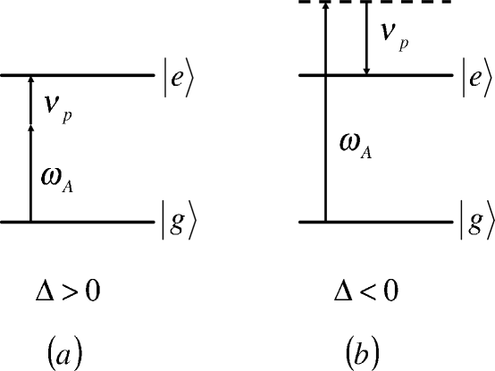
In the case that $\Delta>0$, the laser is detuned below the atomic transition, which we refer to as red detuning. We can resonantly excite so called red sidband transitions when $\Delta\approx n\nu_{p}$. Near such a resonance ($n=1$) we can make the rotating wave approximation and describe the interaction by the Hamiltonian

$$\hat{H}^{(m)}_{I}=\imath\frac{\Omega_{0}\eta}{\sqrt{N}}\sum_{p=1}^{N}s^{(p)}_{m}\left(\hat{a}_{p}\sigma_{+}-\hat{a}_{p}^{\dagger}\sigma_{-}\right)$$ (7)

This describes the usual Jaynes-Cummings model of a two level system interacting with a bosonic degree of freedom. In physical terms it describes a Raman process in which one laser photon and one trap phonon are absorbed to excite the atom (see figure 1). A phonon detector defined this way would respond to the normally ordered moments of the phonon field amplitude.

In the case that $\Delta<0$, the laser is detuned above the atomic transition, which we will refer to as blue detuning. The resonant term for the fisrt blue sideband is then given by

$$\hat{H}^{(m)}_{I}=\imath\frac{\Omega_{0}\eta}{\sqrt{N}}\sum_{p=1}^{N}s^{(p)}_{m}\left(\hat{a}_{p}\sigma_{-}-\hat{a}_{p}^{\dagger}\sigma_{+}\right)$$ (8)

Again this is a Raman process in which the atom is excited by the absorption of one laser photon and the emission of one phonon (see figure 1). Considered as a phonon counter this would correspond to a detector that responded to anti-normally ordered moments of the phonon field amplitude.

Using laser cooling techniques it is possible to cool the system very nearly to the ground state of the vibrational degrees of freedom. In reality this becomes more difficult as the number of ions, and thus normal modes increases. However for our purposes even one ion would suffice. In current experiments the cooling is sufficiently efficient to reach the ground state with probability 0.999LeibfriedB . We thus assume an initial state of the form,

$$\psi(0)\rangle\equiv|\mathbf{0}\rangle=|g\rangle\otimes|0\rangle_{\textrm{vib}}$$ (9)

where the initial vibrational state is a tensor product of the ground states of each of the normal modes,

$$|0\rangle_{\textrm{vib}}=\prod_{n=1}^{p}|0_{p}\rangle\ .$$ (10)

We will exponentially chirp the trap frequency up or down such that

$$\nu\to\nu(t)=e^{\pm\kappa t}$$ (11)

with $\kappa$ the chirp rate and focus our laser on the first ion ($m=1$). For a constant trap frequency the phonon annihilation operator satisfies the usual uncoupled mode equation $\dot{\hat{a}}_{p}(t)=-\imath\nu_{p}\hat{a}_{p}(t)$ with solution $\hat{a}_{p}(t)=\exp(-\imath\nu_{p}t)\,\hat{a}_{p}(0)$, $\nu_{p}=\sqrt{\mu_{p}}\,\nu$ which was used in Eq.(6). For an chirped trap frequency given by Eq.(11) between an initial time $t_{0}$ and final time $t$, the phonon mode now satisfies the following equation of motion, with solution

$$\frac{d}{dt}\hat{a}_{p}(t)=-\imath\nu_{p}e^{\kappa t}\,\hat{a}_{p}(t)\quad\Rightarrow\quad\hat{a}_{p}(t)=\exp\left(\imath\frac{\nu_{p}}{\kappa}e^{\kappa t_{0}}\right)\,\exp\left(-\imath\frac{\nu_{p}}{\kappa}e^{\kappa t}\right)\;\hat{a}_{p}(t_{0}).$$ (12)

where we consider the chirp-up case first (with the chirp down case discussed subsequently).

We now suppose that the coupling to the detector is turned on at the same time as the frequency modulation is turned on, and turned off at the same time as the frequency modulation is turned off. This is a rather different scenario to the usual discussion of the Unruh-Davies effect in which the detector is always coupled to the field and continuously accelerated, ie the red shift frequency modulation is always on.

We are interested in the probability $P_{m}(T,t_{0})$ for the excitation of the $m$’th ion from the ground state to all excited states of detector and field for a detector turned on at $t=t_{0}$ and turned off at $t=T$. The detector in our case has only one excited state. We let the excited states of the vibrational degree of freedom be represented by a complete orthonormal basis $|\phi_{\alpha}\rangle$. The total excitation probability is then note1

$$P_{m}(T,t_{0})=\chi^{2}\int_{t_{0}}^{T}dt^{\prime}\int_{t_{0}}^{T}dt^{\prime\prime}e^{i\Delta(t^{\prime}-t^{\prime\prime})}G(t^{\prime},t^{\prime\prime})$$ (13)

where the field correlation function is defined as

$$G(t^{\prime},t^{\prime\prime})=\hskip 2.5pt_{\textrm{vib}}\langle 0|\hat{q}_{m}(t^{\prime})\hat{q}_{m}(t^{\prime\prime})|0\rangle_{\textrm{vib}}$$ (14)

with the field now given by

$$\hat{q}_{m}(t)=\frac{i}{\sqrt{N}}\sum_{p=1}^{N}s^{(p)}_{m}\left(\hat{a}_{p}e^{-i\frac{\nu_{p}}{\kappa}e^{\kappa t}}-\hat{a}_{p}^{\dagger}e^{i\frac{\nu_{p}}{\kappa}e^{\kappa t}}\right)\ ,$$ (15)

and we have neglected the phase factor arising from the initial time as it does not contribute to the correlation function. Substituting this result into Eq.(14),

$$P_{m}(T,t_{0})=\chi^{2}\sum_{p=1}^{N}\frac{|b_{m}^{(p)}|^{2}}{\sqrt{\mu_{p}}}|I_{p}(T,t_{0})|^{2}$$ (16)

where the integral is

$$I_{p}(T,t_{0})\equiv\int_{t_{0}}^{T}\,dt\,e^{\imath\Delta t}e^{\left(\imath\frac{\nu_{p}}{\kappa}\,e^{\kappa t}\right)}.$$ (17)

With no loss of generality we may now set $t_{0}=0$. We first consider the case $\Delta>0$, which is the red-sideband case. Our objective is to calculate the excitation probability for the two level system near the red sideband transition which we label $P_{m}^{R}(T,t_{0})$.

To evaluate this integral we first change to dimensionless time, $\tau=\kappa t$, so that

$$I_{p}(T,t_{0})=\frac{1}{\kappa}\int_{0}^{\kappa T}\,d\tau\,e^{\imath a\tau}e^{\imath b\,e^{\tau}}.$$ (18)

where $a=\Delta/\kappa$ and $b=\nu_{p}/\kappa$. Next we define the constant $\alpha$

$$b=e^{-\alpha}$$ (19)

It then seems sensible to make the new change of variable $\tau^{\prime}=\tau-\alpha$ so that the integral becomes

$$\frac{e^{ia\alpha}}{\kappa}\int_{-\alpha}^{\kappa T-\alpha}d\tau e^{ia\tau}e^{ie^{\tau}}$$ (20)

In an experiment one needs to vary $\Delta$ near the red or blue sideband, so we expect that $\Delta$ and $\nu_{p}$ are of the same order. We now consider the limit in which $\nu_{p}/\kappa<<1$ for all the normal modes. In this limit $\alpha>>1$, the integral does not depend much on $\alpha$, so we extend the lower limit of the integral to infinity. Furthermore we suppose the time over which the detector and modulation are on is such that $T>>\nu_{p}$, in which case the integral does not vary much with $T$. In that case we can extend the upper limit of the integral to infinity, so that

$$I_{p}\approx\frac{e^{ia\alpha}}{\kappa}\int_{-\infty}^{\infty}d\tau e^{ia\tau}e^{ie^{\tau}}$$ (21)

Changing the variable of integration to $y=e^{\tau}$ we obtain an expression for $I_{p}$ with arbitrary limits as

$$I_{p} = \frac{e^{ia\alpha}}{\kappa}\int_{0}^{\infty}dyy^{ia-1}e^{iy}$$ (22)

$$= \frac{e^{ia\alpha}}{\kappa}\Gamma(ia)e^{-\pi a/2}$$ (23)

If we now use the identity $|\Gamma(ix)|^{2}=\pi/[x\sinh(\pi x)]$ for real $x$ GR we see that

$$|I_{p}|^{2}=\frac{2\pi}{\kappa\Delta}\frac{1}{e^{2\pi\Delta/\kappa}-1}$$ (24)

Inserting this into Eq.(16) we can write $P_{m}^{R}$ in the suggestive form

$$P_{m}^{R}=\frac{\Omega_{0}^{2}\eta^{2}}{\kappa\Delta}\;\frac{2\pi}{e^{\hbar\Delta/k_{B}T}-1}\;\sum_{p=1}^{N}\frac{|b_{1}^{(p)}|^{2}}{\sqrt{\mu_{p}}}$$ (25)

where we have defined the Unruh temperature as

$$k_{B}T\equiv\frac{\hbar\kappa}{2\pi}.$$ (26)

Eq.(25) has the analogous form to a thermal spectrum at temperature $T$ as seen by a uniformly accelerated observer moving through a particle-free inertial vacuum. The ”thermal” form of the probability is independent of the phonon frequencies $\nu_{p}$ since we have taken the upper limit $t$ to infinity. The last summation expression is just a numerical factor, which can be computed DJ , or dropped in the case of a single ion in the trap.

The analogy with the Unruh effect BD for a uniformly accelerated observer in Minkowski space can be seen as follows. As discussed in alsing_milonni the chirping of the trap frequencies can be considered as arising from the the modification of the usual Minkowski plane wave $\exp(i\varphi_{\pm})\equiv\exp\big{(}i(kz\pm\omega t)\big{)}$ due to the motion of the accelerated observer. For an observer moving at constant velocity $v_{0}$ in Minkowski space, a Lorentz transformation (LT) of the phase $\varphi_{\pm}$ viz $ct^{\prime}=ct\cosh r+z^{\prime}\sinh r$ and $z^{\prime}=z\cosh r+ct^{\prime}\sinh r$ with the rapidity defined by $\tanh r=v_{0}/c$, simply transforms it to $\varphi_{\pm}\to\varphi^{\prime}_{\pm}=(\omega/c)e^{\pm r}\,(z^{\prime}\pm ct^{\prime})\equiv(\omega^{\prime}/c)\,(z^{\prime}\pm ct^{\prime})$ which merely produces the constant doppler shifted frequencies in the new frame $\omega^{\prime}=\omega e^{\pm r}$. For an accelerated observer, one has to perform a time dependent LT at each instant to the comoving frame that is instantaneously at rest with respect to the accelerated observer. The orbit of the accelerated (Rindler) observer as described by an inertial Minkowski observer is given by the Rindler transformation $ct(\tau)=(c^{2}/a)\,\sinh(a\tau/c)$ and $z(\tau)=(c^{2}/a)\,\cosh(a\tau/c)$ where $a$ is the constant uniform acceleration. Under this transformation, the Rindler observer experiences phase of the Minkowski plane wave $\exp(i\varphi_{\pm})$ as transformed to $\varphi_{\pm}\to\varphi_{\pm}(\tau)=kz(\tau)\pm\omega t(\tau)=(\omega c/a)\,e^{\pm a\tau/c}$. These are the chirped frequencies that appear in Eq.(17) in exponentially expanding or contracting the trap. The Fourier transform of this modified plane wave with respect to the Rindler proper time $\tau$ can be considered as a measure of the noise spectrum seen by the accelerated observer viz

$$S(\Delta)=\left|\int_{-\infty}^{\infty}\,dt\,e^{\pm\imath\Delta\tau}e^{\left(i\omega c/a\,e^{\pm a\tau/c}\right)}\right|^{2}=\left|\displaystyle\frac{(e^{\pm i\pi/2})^{\pm i\Delta c/a}}{(\frac{\omega c}{a})^{\pm i\Delta c/a}}\;\Gamma\left(\pm i\frac{\Delta c}{a}\right)\right|^{2}=\frac{2\pi c}{\Delta a}\;\displaystyle\frac{1}{e^{i\Delta c/a}-1},$$ (27)

analogous to $|I_{p}(\infty,-\infty)|^{2}$ as in Eq.(24). Here the perceived thermal temperature is defined from the only other frequency that can be formed from the Rindler observers accelerated motion, $a/c$. Thus we get the usual Unruh temperature defined by $T=\hbar a/2\pi c$. In our ion trap analogy, the role of the acceleration frequency $a/c$ is played by the trap expansion rate $\kappa$.

Figure 1: Energy Level Diagrams. Tuning to (a) red side band, $\Delta\equiv\omega_{A}-\omega_{L}=\nu_{p}>0$, (b) blue side band $\Delta=-\nu_{p}<0$. The Unruh effect Eq.(25) takes place on the red sideband. We obtain an anti-normally ordered Unruh effect if we tune to the blue side band.

Figure 2: Vibrational Resonances. Red (a) and blue (b) vibrational sidebands corresponding to the energy level diagrams in Fig.(1).

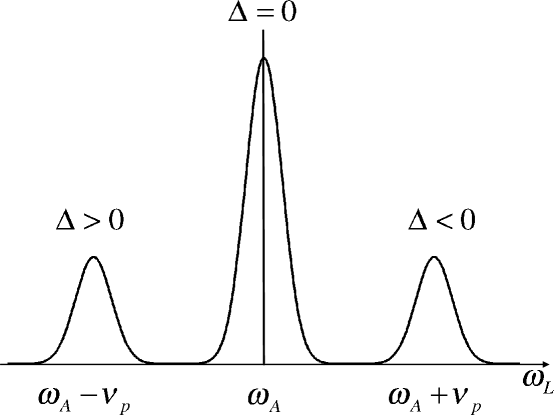
It is important to note that in order to obtain the Planck factor $(e^{2\pi\Delta/\kappa}-1)^{-1}$ in Eq.(24), indicative of a Bose-Einstein (BE) thermal distribution and the signature of the Unruh effect, we made crucial use of a positive detuning $\Delta>0$, corresponding to a red sideband detuning in Fig.(1) and Fig.(2). This resulted in the factor $(i)^{i\Delta/\kappa}=\big{(}e^{i\pi/2}\big{)}^{i\Delta/\kappa}=e^{-\pi\Delta/2\kappa}$ that appears in $I_{p}$ in Eq.(23). Dividing the square of this factor into the $\sinh$ function appearing in the denominator of $|I_{p}|^{2}$, resulting from the term $|\Gamma(i\Delta/\kappa)|^{2}$, produces the signature BE thermal distribution function.

If on the other hand, we had instead chosen $\Delta=-|\Delta|<0$ corresponding to a negative detuning to the blue side band Fig.(2)b, the previous factor would become $\big{(}e^{i\pi/2}\big{)}^{-i|\Delta|/\kappa}=e^{\pi|\Delta|/2\kappa}$. Dividing the square of this term into the $\sinh$ function appearing in the denominator then produces alternatively the probability for excitation on the blue sideband

$$P_{m}^{B}=\frac{\Omega_{0}^{2}\eta^{2}}{\kappa|\Delta|}\;\frac{2\pi}{1-e^{-2\pi|\Delta|/\kappa}}\;\sum_{p=1}^{N}\frac{|b_{1}^{(p)}|^{2}}{\sqrt{\mu_{p}}},$$ (28)

with the same definition of the Unruh temperature as in Eq.(26).

We might label such a distribution an anti-normally ordered Unruh effect since the vibrational excitation from the ground to the excited state takes place by an absorption of a photon and an emission of a phonon to the electronic state $|e\rangle$ as depicted in Fig.(1)b, i.e. by a term such as $\hat{a}_{p}\,\sigma_{-}$, see Eq.(8). As discussed earlier, such a detector responds to the anti-normally ordered moments of the phonon field amplitude. Note that as $\kappa\to 0$ ($T\to 0$) in Eq.(28) we get a finite contribution to the probability for excitation $P_{m}$. In the case of red sideband detuning, the usual Unruh effect analogy in Eq.(25), $P_{m}\to 0$ as $\kappa\to 0$. This limit corresponds to a fixed trap frequency $\nu$ for which we get no excitation as described above.

The above $\kappa\to 0$ limiting cases can also be understood as follows. For a constant trap frequency $\nu_{p}(t)=\nu_{p}$ the relevant integral to compute is

$$I_{p}(\infty,-\infty)=\int_{-\infty}^{\infty}\,dt\,e^{i\Delta t}\,e^{i\nu_{p}t}=2\pi\delta(\Delta+\nu_{p})$$ (29)

which arises from the $\hat{a}_{p}^{\dagger}\sigma_{+}$ term in $\hat{H}^{(m)}_{I}$ Eq.(5) when acting on the motionally cooled ground state Eq.(9). For blue sideband detuning $\Delta=-|\Delta|<0$ we obtain a non-zero contribution from the delta function. In the usual ion trap excitation schemes for quantum computing wineland , the resonant (rotating wave approximation) portion of the Hamiltonian Eq.(5) gives rise to the anti-Jaynes-Cummings type interaction Eq.(8), which permits transitions of the form $|n\rangle|g\rangle\to|n+1\rangle|e\rangle$. With our motionally cooled ground state Eq.(9) with $n=0$ such transitions are possible from $|0\rangle|g\rangle\to|1\rangle|e\rangle$. Thus $\hat{a}_{p}^{\dagger}\sigma_{+}$ represents a resonant contribution to the Hamiltonian.

For red sideband detuning, $\Delta>0$ we do not obtain a contribution from the delta function. Here the resonant portion of the Hamiltonian Eq.(5) gives rise to the usual Jaynes-Cummings type interaction Eq.(7), which permits transitions of the form $|n\rangle|g\rangle\to|n-1\rangle|e\rangle$. With an initial motional ground state Eq.(9) with $n=0$ such transitions are not possible. However, in writing down Eq.(7) we have dropped the non-resonant anti-normally ordered terms. It is the $\hat{a}_{p}^{\dagger}\sigma_{+}$ non-RWA term in $\hat{H}^{(m)}_{I}$ Eq.(5) that can produce transitions from the motionally cooled ground state Eq.(9) and is responsible for the Unruh-like behavior of the probability $P_{m}$ for excitation out of this ground state.

We can also give an Unruh analogy interpretation of the zero contribution to the delta function $\delta(\Delta+\nu_{p})$ in Eq.(29). The case of red sideband detuning $\Delta>0$, a constant trap frequency is analogous to an inertial observer moving with constant velocity in Minkowski space, giving rise to a constant Lorentz transformation as discussed above. For a constant velocity observer, an inertial detector would have a response function proportional to $\delta(E+E_{0})$ where $E\;(\textrm{analogously}\;\Delta)$ is the energy of the detected particle and $E_{0}>0\;(\textrm{analogously}\;\nu_{p})$ represents the atomic transition frequency producing the particle to be detected BD . Since the detector only responds to positive energies $E>0$, the contribution from the delta function $\delta(E+E_{0})$ is zero, which simply states that an inertial detector moving through the Minkowski vacuum would detect no particle production.

III Finite Chirp, General Expression

For a finite chirp between times $t_{0}$ and $T$ we can develop a general expression for $P_{m}(T,t_{0})$ in terms of the incomplete gamma functions $\gamma(\mu,x)=\int_{0}^{x}dt\;t^{\mu-1}e^{-t}$ and $\Gamma(\mu,x)=\int_{x}^{\infty}dt\;t^{\mu-1}e^{-t}$ such that $\gamma(\mu,x)+\Gamma(\mu,x)=\Gamma(\mu)$. Let us write $\int_{y_{0}}^{y_{T}}dy=\int_{0}^{\infty}dy-\int_{0}^{y_{0}}dy-\int_{y_{T}}^{\infty}dy$ for general finite duration limits in Eq.(22) with the definitions $y_{0}=e^{\kappa t_{0}}$ and $y_{T}=e^{\kappa T}$. By scaling the integration variable to $y=y_{0}x$ in the second integral on the right hand side and $y=y_{T}x$ in the third integral on the right hand side one can easily show that

$$I_{p}(T,t_{0})=\frac{1}{\kappa}\,\displaystyle\frac{\Gamma(ia)\left(e^{i\frac{\pi}{2}}\right)^{ia}}{a^{ia}}\Big{(}1-\gamma^{\prime}(ia,-iby_{0})-\Gamma^{\prime}(ia,-iby_{T})\Big{)},$$ (30)

with the same definitions of $a$ and $b$ used in Eq.(22), and where we have defined the normalized gamma functions $\gamma^{\prime}(\mu,x)=\gamma(\mu,x)/\Gamma(\mu)$ and $\Gamma^{\prime}(\mu,x)=\Gamma(\mu,x)/\Gamma(\mu)$ such that $\gamma^{\prime}(\mu,x)+\Gamma^{\prime}(\mu,x)=1$. Thus we obtain

$$P_{m}(T,t_{0})=\frac{\Omega_{0}^{2}\eta^{2}}{\kappa\Delta}\;\frac{2\pi}{e^{\hbar\Delta/k_{B}T}-1}\;\sum_{p=1}^{N}\left|1-\gamma^{\prime}\left(i\frac{\Delta}{\kappa},-i\frac{\nu_{p}}{\kappa}e^{\kappa t_{0}}\right)-\Gamma^{\prime}\left(i\frac{\Delta}{\kappa},-i\frac{\nu_{p}}{\kappa}e^{\kappa T}\right)\right|^{2}\frac{|b_{1}^{(p)}|^{2}}{\sqrt{\mu_{p}}}.$$ (31)

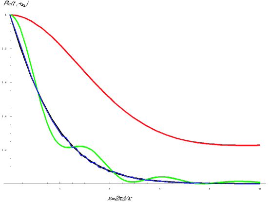
The previous expression for the total excitation probability in Eq.(25) corresponds to $P_{m}(\infty,-\infty)$ using Eq.(31) above which formally corresponds to sweeping the trap frequency from an initial zero value to an infinite final value. Considering a more realistic situation applicable to experiments, let us consider $t_{0}=0$ and a finite trap expansion time $T$, which corresponds to sweeping the trap frequency from $\nu\to\nu e^{\kappa T}$. Considering Eq.(31) as a function of the detuning $\Delta$ with parameters $\nu_{p}/\kappa$ and $\kappa T$ we can recover Eq.(25) under the following conditions

$$\frac{\nu_{p}}{\kappa}\ll 1,\qquad\frac{\nu_{p}}{\kappa}e^{\kappa T}\gg 1\qquad\forall\,p=(1,2,\ldots,N)$$ (32)

which makes the incomplete gamma functions small compared to unity. As an example, taking $\nu_{p}/\kappa=0.01$ and $(\nu_{p}/\kappa)\exp(\kappa T)=100$ requires that $\kappa T>9.2$

Note that Eq.(31) approaches $P_{m}(\infty,-\infty)$ of Eq.(25) as $t_{0}\to-\infty$ and $T\to\infty$ in which the incomplete gamma functions approach zero. The main point for experimental purposes is that we only need to take finite limits of the order $\nu_{p}/\kappa\sim 10^{-2}$ and $(\nu_{p}/\kappa)\exp(\kappa T)\sim 10^{2}$ to approximate the full Unruh case, $P_{m}(\infty,-\infty)$ as shown in Fig.(3).

Figure 3: Finite duration chirp: Plot of Eq.(31) for $p=1$ and $\Omega_{0}\eta/\kappa=1$, $\nu_{p}/\kappa=1$ with $x=2\pi\Delta/\kappa$ as the abscissa and $P_{m}(t,-\infty)$ as the ordinate for various values of $y_{t}=e^{\kappa T}=\nu_{1}(T)/\nu$; red curve $y_{T}=1$, green curve $y_{T}=10$, blue curve $y_{T}=100$. The smooth black curve is the pure Unruh case $P_{m}(\infty,-\infty)$ given by Eq.(25).

IV Discussion and conclusion.

As we have shown, the experimental signature of the exponential modulation of the trap frequency is the Planck-like form for the excitation probability for the two level electronic system in each ion. In such experiments it is the ratio of the excitation probability on the red ($\Delta=\nu$) and blue ($|\Delta|=\nu$)sidebands that is determined:

$$R_{e}=\frac{P_{m}^{R}}{P_{m}^{B}}$$ (33)

as this number is independent of the Rabi frequency, the Lamb-Dicke parameter, and the time of interaction between the vibrational and electronic degrees of freedomMonroe95 ; Turchette2000 . Let us consider the case of a single ion with trap frequency $\nu$. Using Eqs.(25,28) we see that

$$R=\frac{1-e^{-2\pi\nu/\kappa}}{e^{2\pi\nu/\kappa}-1}$$ (34)

In a typical experiment one can detect $R$ values as low as $0.05$ with about $20$% error. This implies that $\nu/\kappa\approx 0.5$. At secular frequencies of $\nu/2\pi=0.1\ -\ 1$ MHz, we need a modulation frequency of the order of a few hundred Khz to MHz; a not particularly difficult requirement for fast electronics.

The key issue however is the absolute size of the excitation probabilities at the red and blue sideband. This is determined by the prefactor $(\Omega_{0}\eta)^{2}/(\kappa\nu)$. Defining

$$z=2\pi\nu/\kappa$$ (35)

the equations for the excitation probability at the red and blue sidebands are

$$P^{R} = \left(\frac{\Omega_{0}\eta}{\nu}\right)^{2}\frac{z}{e^{z}-1}$$ (36)

$$P^{B} = \left(\frac{\Omega_{0}\eta}{\nu}\right)^{2}\frac{z}{1-e^{-z}}$$ (37)

As we expect $z$ to be of the order of unity, we require that the secular frequency is within one order of magnitude of the effective Rabi frequency. This corresponds to a rather weakly bound ion, but should be achievable if stimulated Raman transitions are used to couple the two level system. For example the relevant transition in $\mbox{}9$Be$\mbox{}^{+}$ can have an effective Rabi frequency of the order of $\Omega_{0}/2\pi=500$kHzSackett2000 . If we use the centre of mass mode with secular frequency of $\nu/2\pi=200$kHz, and a Lamb-Dicke parameter of $\eta=0.2$, the prefactor is $0.25$. At a more conservative estimate of $\eta=0.05$, well within the Lamb-Dicke regime, the prefactor drops to a value of $0.015$. These numbers are encouraging enough to suggest the plausibility of observing an analogous Unruh-like effect in today’s linear ion traps.