Dynamics of a Raman coupled model: entanglement and quantum computation

Abstract

The evolution of a Raman coupled three-level $\Lambda$ atom with two quantized cavity modes is studied in the large detuning case; i.e. when the upper atomic level can be adiabatically eliminated. Particularly the situation when the two modes are prepared in initial coherent or squeezed states, with a large average number of photons, is investigated. It is found that the atom, after specific interaction times, disentangles from the two modes, leaving them, in certain cases, in entangled Schrödinger cat states. These disentanglement times can be controlled by adjusting the ratio between average numbers of photons in the two modes. It is also shown how this effective model may be used for implementing quantum information processing. Especially it is demonstrated how to generate various entangled states, such as EPR- and GHZ-states, and quantum logic operations, such as the control-not and the phase-gate.

I Introduction

Entanglement is one of the most striking features of quantum mechanics. It is fundamental for non-locality of quantum mechanics, quantum computing and information processing chuang and much effort has been done, both theoretically and experimentally, in order to achieve a deeper understanding of this property. For a non-zero interaction between the system under consideration and the surrounding environment, information about the system will decohere into the environment, which is one of the main limitations for scalable quantum computing. However, the last two decades have seen great progress in achieving isolated controllable quantum mechanical systems. Cavity quantum electrodynamics provides one such system; an atom is coupled to a quantized electromagnetic field through a dipole-interaction inside a high-Q cavity. The simplest example is described by the Jaynes-Cummings model jc , where a two-level atom interacts with just one mode of the cavity field. This model is, within the rotating wave approximation, analytically solvable and has been widely investigated since it was first introduced. In spite of its simplicity, many interesting purely quantum mechanical phenomena, such as, for example, revivals of Rabi oscillations and field squeezing, may be understood from it. It is, in most cases, easy to generalize the Jaynes-Cummings model to other similar systems, for example, multi-mode fields and multi-level atoms, see the review article genjc . Some of these generalized models can still be solved analytically and in this paper we focus on one of them.

We consider a three-level $\Lambda$-type atom coupled to two non-degenerate cavity modes. By tuning the two transitions off resonance, the upper atomic level can be adiabatically eliminated and the atomic system may be described by an effective two-level atom. The lower atomic levels are thus coupled to each other through the two modes, and in general the three subsystems, mode-mode-atom, become highly entangled. This entanglement can persist even when the photon numbers become large and we would otherwise enter a classical regime.

For the various generalized Jaynes-Cummings models, the classical limit is when the initial cavity modes of interest are prepared in coherent states with a large average number of photons. The behavior of the ordinary Jaynes-Cummings model in this limit was investigated in great detail in GB and it was found that, at particular interaction times, the atom disentangled from the field, independently of its initial atomic state. At these disentanglement times the field is in a so-called Schrödinger cat state, that is a superposition of two states macroscopically far apart. The interaction splits the initial coherent state into two parts in phase space, which at the disentanglement times differ in phase by an angle $\pi$. The theory outlined in GB has recently also been demonstrated experimentally haroche . These Schrödinger cat states are well suited for the study of how decoherence depends on the ”size” of the system, quantum information is supposed to be lost more rapidly to the environment the more classical the system is. The quantum mechanical superposition then collapses into a statistical mixture of the two parts, see reference collapse .

The classical limit in our model has been investigated in kines . However, reference kines did not investigate the generation of particular states of the two modes, but looked at the amount of mode-entanglement in special cases. We will show that, for some initial states of the two modes with large average of photons, the atom will disentangle from the modes and that the modes are in entangled Schrödinger cat states at these times. These states are in one sense more non-classical than the Schrödinger cat states generated in the ordinary Jaynes-Cummings model, since the two modes are also entangled with each other. These states may be used, for example, to investigate decoherence and also to check ‘non-locality’ of quantum mechanics. We find that the disentanglement times and the form of the Schrödinger cat states depend on the ratio between the average number of photons in the two modes. A consequence of this is that the disentanglement time may be small in the classical limit, which differs from the ordinary Jaynes-Cummings model where this time goes as the square root of the average of photons. So, the theory predicts that the atom will disentangle from the modes at a certain time and that the modes and the atom are then in some specific states. Thus, by measuring the atomic state at this time we achieve a direct confirmation that the process of generating entangled Schrödinger cat states was successful. The outcome of the atomic measurement gives us a check, and makes the preparation scheme more robust.

In section II we present the model and give the general analytical solution and also some of its properties. In the following section III, the ideas from reference GB about the classical limit are applied to our system: we then derive the atomic disentanglement times and approximate expressions for the field state. The validity of the approximations are also investigated by calculating the purity of the separate modes. It is found that initial coherent states are not sharp enough, in terms of uncertainties in photon numbers, in order to prepare the entangled Schrödinger cat states. In section IV we give examples of several quantum logic gates and examples of entangled states achievable through the model. Finally we conclude the paper in section V with a summary.

II The model

We consider a three-level $\Lambda$-atom, with lower levels $|a\rangle$, $|b\rangle$ and upper level $|c\rangle$, interacting with two non-degenerate microwave modes. The energies of the respective atomic levels and field modes are: $\hbar\Omega_{a,b,c}$ and $\hbar\omega_{1,2}$. The states $|b\rangle$ and $|a\rangle$ couple to the state $|c\rangle$ through a dipole interaction with modes one and two respectively. In the situation

$$\hbar\Delta=\hbar(\Omega_{c}-\Omega_{b})-\hbar\omega_{1}=\hbar(\Omega_{c}-\Omega_{a})-\hbar\omega_{2},$$ (1)

see figure 1, the population in state $|c\rangle$ can be adiabatically eliminated provided that the detuning $\Delta$ is large; see reference bose . The atom-field evolution, after the elimination, is then governed by the effective Hamiltonian ($\hbar=1$)

$$H=g(a_{2}^{\dagger}a_{1}\sigma^{-}+a_{2}a_{1}^{\dagger}\sigma^{+}),$$ (2)

in the dipole and the rotating wave approximations. Here the $a_{1,2}$’s are the boson operators for the two modes, $\sigma^{+}=|b\rangle\langle a|$, $\sigma^{-}=|a\rangle\langle b|$ and the effective coupling is $g=g_{ac}g_{bc}/\Delta$ with $g_{ij}$ being the original dipole couplings between the corresponding atomic levels (here $g_{ab}=0$). With the Hamiltonian (2), the number of excitations in the two modes, $N=a_{1}^{\dagger}a_{1}+a_{2}^{\dagger}a_{2}$, is clearly conserved. This symmetry can be used, for example, to calculate the atomic inversion for special cases, as is shown below.

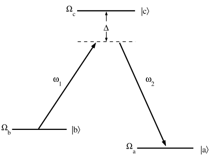
Figure 1: Energy level diagram of the three-level $\Lambda$-atom. The detuning $\Delta$ is assumed to be large so that the atomic level $|c\rangle$ can be eliminated. The two mode frequencies are represented by $\omega_{1}$ and $\omega_{2}$.

A general disentangled initial state of the system, excluding the upper state $|c\rangle$, can be written as

$$|\Psi(0)\rangle=\sum_{n,m}C_{n}^{(1)}C_{m}^{(2)}|n,m\rangle\left[\gamma|a\rangle+\delta|b\rangle\right],$$ (3)

where $|n,m\rangle$ refers to $n$ photons in mode one and $m$ photons in mode two. After a time $t$ the state will evolve into

$$\begin{array}[]{ccl}|\Psi(t)\rangle&=&\sum_{n,m}C_{n}^{(1)}C_{m}^{(2)}\left\{\gamma\left[\cos(gt\sqrt{(n+1)m})|n,m,a\rangle\right.\right.\\ \\ &&\left.-i\sin(gt\sqrt{(n+1)m})|n+1,m-1,b\rangle\right]\\ \\ &&+\delta\left[\cos(gt\sqrt{(m+1)n})|n,m,b\rangle\right.\\ \\ &&\left.\left.-i\sin(gt\sqrt{(m+1)n})|n-1,m+1,a\rangle\right]\right\}.\end{array}$$ (4)

Here it is understood that the states $|n,m,a\rangle\equiv|n,m\rangle|a\rangle$ and $|n,m,b\rangle\equiv|n,m\rangle|b\rangle$.

Using the above expression (4), the atomic inversion becomes

$$\begin{array}[]{lll}W(t)&=&\langle\Psi(t)|\sigma_{z}|\Psi(t)\rangle\\ \\ &=&\sum_{n,m}\left[|C_{n}^{(1)}|^{2}|C_{m}^{(2)}|^{2}|\gamma|^{2}\cos^{2}(gt\sqrt{(n+1)m})\right.\\ \\ &&+|C_{n+1}^{(1)}|^{2}|C_{m-1}^{(2)}|^{2}|\delta|^{2}\sin^{2}(gt\sqrt{(n+1)m})\\ \\ &&-|C_{n}^{(1)}|^{2}|C_{m}^{(2)}|^{2}|\delta|^{2}\cos^{2}(gt\sqrt{(m+1)n})\\ \\ &&\left.-|C_{n-1}^{(1)}|^{2}|C_{m+1}^{(2)}|^{2}|\gamma|^{2}\sin^{2}(gt\sqrt{(m+1)n})\right].\end{array}$$ (5)

An interesting observation is that if the photon-distributions of the two modes is identical, $|C_{n}^{(1)}|=|C_{m}^{(2)}|,\,\,\,n=m$, the inversion is strictly zero in the case when $|\gamma|=|\delta|$. This does not, however, mean that the atom is not entangled with the field-modes, as we will see in the next section. This phenomenon, as mentioned above, is a consequence of the symmetry in the system; for equal field intensities, population transfer is equally likely in both directions between the two atomic states. The ordinary Jaynes-Cummings model does not have this symmetry. Note that we have assumed the two modes to be initially disentangled, but the result holds also for entangled modes as long as the two modes have equal photon-distributions. Another example of atomic population trapping in the Raman model is studied in atomtrap . There, one particular state of the field is found, such that the inversion $W(t)$ is constant for any initial atomic state.

III Evolution for large initial fields

III.1 Atom-field disentanglement

Following the method in GB we now investigate the behavior of the combined atom-field system when both the initial fields of the modes are large. This situation has been investigated in reference kines . However, in reference kines only some specific cases of the evolution of the system where studied, and reference kines did not discuss how it may be used for state preparation.

We assume the two photon number distributions to be peaked around the average photon numbers $\bar{n}$ and $\bar{m}$ and further, in the large photon limit, $\bar{n},\bar{m}\gg 1$, we replace $C_{n\pm 1}^{(1)}C_{m\mp 1}^{(2)}$ by $C_{n}^{(1)}C_{m}^{(2)}e^{i\varphi_{nm}^{(\pm)}}$. We also put the phase to be constant, $\varphi_{nm}^{(\pm)}=\pm\varphi$, under the assumption that the phases of the two fields are slowly varying around the average photon numbers. For large initial fields, the state (4) can then, with the above approximations, be written as

$$\begin{array}[]{lll}|\Psi(t)\rangle&\approx&\sum_{n,m}C_{n}^{(1)}C_{m}^{(2)}\left\{\left[\gamma\cos(gt\sqrt{(n+1)m})\right.\right.\\ \\ &&\left.-i\delta e^{i\varphi}\sin(gt\sqrt{(n+1)m})\right]|n,m,a\rangle\\ \\ &+&\left[\delta\cos(gt\sqrt{(m+1)n})\right.\\ \\ &&\left.\left.-i\gamma e^{-i\varphi}\sin(gt\sqrt{(m+1)n})\right]|n,m,b\rangle\right\}.\end{array}$$ (6)

We introduce the new orthogonal atomic basis states $|\phi_{\pm}\rangle=\frac{1}{\sqrt{2}}(e^{i\varphi}|a\rangle\pm|b\rangle)$, and using (6) with $\gamma=\frac{1}{\sqrt{2}}e^{i\varphi}$ and $\delta=\frac{1}{\sqrt{2}}$ we find for these states

$$\begin{array}[]{lll}|\Psi(t)\rangle_{\pm}&\approx&\frac{1}{\sqrt{2}}\sum_{n,m}C_{n}^{(1)}C_{m}^{(2)}e^{\mp igt\sqrt{(m+1)n}}\times\\ \\ &&\left[e^{i\varphi}e^{\pm igt\left[\sqrt{(m+1)n}-\sqrt{(n+1)m}\right]}|a\rangle\pm|b\rangle\right]|n,m\rangle\\ \\ &\approx&\frac{1}{\sqrt{2}}\left(e^{i\varphi}e^{\pm i\frac{gt}{2}\left(\sqrt{\frac{\bar{n}}{\bar{m}}}-\sqrt{\frac{\bar{m}}{\bar{n}}}\right)}|a\rangle\pm|b\rangle\right)\times\\ \\ &&\sum_{n,m}C_{n}^{(1)}C_{m}^{(2)}e^{\mp igt\sqrt{(m+1)n}}|n,m\rangle\\ \\ &=&\frac{1}{\sqrt{2}}\left(e^{i\varphi}e^{\pm i\frac{gt}{2}\left(\frac{\kappa-1}{\sqrt{\kappa}}\right)}|a\rangle\pm|b\rangle\right)|\psi_{\mp}\rangle.\end{array}$$ (7)

In the second step we have made the approximation

$$\sqrt{(m+1)n}-\sqrt{(n+1)m}\approx\frac{1}{2}\left(\sqrt{\frac{\bar{n}}{\bar{m}}}-\sqrt{\frac{\bar{m}}{\bar{n}}}\right),$$ (8)

assuming the photon-distributions to be highly peaked around their averages and that $\bar{n},\bar{m}\gg 1$. The last step defines the field states $|\psi_{\pm}\rangle$ and the parameter $\kappa=\bar{n}/\bar{m}$ as the ratio between the average photon numbers of the two modes.

For effective interaction times

$$\begin{array}[]{lc}gt_{0}^{(j)}=(2j+1)\frac{\pi\sqrt{\kappa}}{|\kappa-1|},&j=0,1,2,...\end{array}$$ (9)

the two atomic parts in equation (7) become equal. Thus, since any initial atomic state can be written as a linear combination of the two orthogonal states $|\phi_{\pm}\rangle$, the atomic state will always disentangle from the field state at these times. So, the interaction, in the large photon limit, describes a non-unitary evolution in the Hilbert-space of the atom GB . However, this disentanglement between the atom and the field, $|\Psi(gt=gt_{0}^{(j)})\rangle=|\psi_{atom}\rangle\otimes|\psi_{field}\rangle$, only occurs if $\kappa\neq 1$. Note, by adjusting the ratio between the average photon numbers in the two modes, varying $\kappa$, it is possible to control the disentanglement time.

A measure of the degree of entanglement between different subsystems is the purity defined as $P_{A}(t)=\mathrm{Tr}\left(\rho_{A}(t)^{2}\right)$. Here $\rho_{A}(t)$ is the reduced density operator for system $A$, obtained by tracing out the other subsystems’ degrees of freedom from the full system’s density operator, $\rho_{A}(t)=\mathrm{Tr}_{B}\left(\rho(t)\right)$. In reference GB , for the ordinary Jaynes-Cummings model, the field was assumed to be in coherent states. However, for a sharper distribution the agreement between the large field approximations and the exact results is supposed to be enhanced, which is also shown in knight . We will assume the initial states of the two modes to be either in coherent or squeezed coherent states. For a coherent state $|\nu\rangle=D(\nu)|0\rangle$, where $D(\nu)=\exp\left(\nu a^{\dagger}-\nu^{*}a\right)$ is the displacement operator, we have

$$C_{n}^{(1)}=e^{-|\nu|^{2}/2}\frac{\nu^{n}}{\sqrt{n!}}$$ (10)

and similarly for mode two

$$C_{m}^{(2)}=e^{-|\mu|^{2}/2}\frac{\mu^{m}}{\sqrt{m!}}.$$ (11)

For a squeezed coherent state $|r,\nu\rangle=S(r)|\nu\rangle$, where $S(r)=\exp\left(r(a^{2}-a^{\dagger 2})/2\right)$, the coefficients are given by knight

$$C_{n}^{(1)}\!=\!\frac{\tanh(r)^{n/2}}{\sqrt{n!\,2^{n}\cosh(r)}}e^{-|\nu|^{2}(1-\tanh(r))/2}H_{n}\!\!\left(\frac{\nu}{\sqrt{\sinh(2r)}}\right)\!,$$ (12)

if $\nu$ is chosen real and $H_{n}$ is the $n$’th Hermite polynomial and, of course, we have a similar result for mode two. In the following, for convenience, we always choose the phases of the initial fields to be zero. Figure 2 shows the atomic purity, $\mathrm{Tr}\left(\rho_{A}(t)^{2}\right)$, as a function of the effective interaction time, both for initial coherent states (dashed curve) and squeezed coherent states (solid line). The reduced atomic density operator is achieved from equation (4), by constructing the full systems density operator and then trace over the two modes degrees of freedom, as mentioned above. In both cases we have $\bar{n}=|\nu|^{2}=150$ and $\bar{m}=|\mu|^{2}=50$, the squeezing parameters for the solid curve are $r_{1}=r_{2}=1$ for both modes and the initial atomic state is $|a\rangle$. It is clear that in the squeezed case, when the photon-distribution is sharper (sub-Poissonian), the disentanglement of the atom is improved. This is most prominent for larger disentanglement times $gt_{0}^{(j)}$. For $j=0$ the atomic purity is almost the same for the two cases; solid and dashed curves. The additional peaks at around $gt\approx 11$ and $gt\approx 22$, seen in the figure, are due to the disentanglement at the revival times; see reference zaheer . This phenomenom is not predicted by the theory given above, see equation (9).

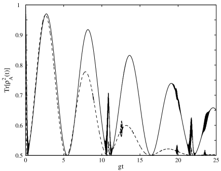
Figure 2: This figure shows the atomic purity as a function of the effective interaction time when the atom is initially in the state $|a\rangle$ and two modes either in coherent states (dashed curve) or squeezed states (solid curve). The average numbers of photons are $\bar{n}=150$ and $\bar{m}=50$ in both cases and the squeezing parameters are $r_{1}=r_{2}=1$, see equation (12). The atom disentangles from the field when the purity equals unity. It is clear the the amount of disentanglement improves for the sub-Poissonian squeezed states, especially at larger times. The sharp peaks at around $gt\approx 11$ and $gt\approx 22$ are the separation of the atom from the field at the revival times.

III.2 Field states at the disentanglement time

We have seen that at certain times $gt_{0}^{(j)}$ given by equation (9), the state of the whole system can be written as a product of the atomic state and the field state in the large photon approximation. The state of the two modes will at these times be a linear superposition of the states $|\psi_{\pm}\rangle$, where the coefficients are determined from the initial atomic state. For an atom initially in the state $|a\rangle$ we obtain, for example,

$$|\psi_{field}(gt_{0}^{(j)})\rangle=\frac{1}{N}\left(|\psi_{+}(gt_{0}^{(j)})\rangle+|\psi_{-}(gt_{0}^{(j)})\rangle\right),$$ (13)

where $N$ is a normalization constant.

As in section III.1 we try to make use of the sharpness of the photon-distributions when the average photon numbers becomes large in order to approximate the expressions for the field states $|\psi_{\pm}\rangle$. If we assume the fields to be initially in coherent states and expand $\sqrt{(m+1)n}$ to first order around $\bar{n}$ and $\bar{m}$ and make use of $\bar{n},\bar{m}\gg 1$, the states become

$$|\psi_{\pm}(t)\rangle\approx e^{\pm i\frac{\sqrt{\kappa}gt}{2}}|\nu e^{\pm i\frac{gt}{2\sqrt{\kappa}}}\rangle|\mu e^{\pm i\frac{\sqrt{\kappa}gt}{2}}\rangle.$$ (14)

At the first disentanglement time $gt_{0}^{(0)}$ we get

$$|\psi_{\pm}(gt_{0}^{(0)}\rangle\approx e^{\pm i\frac{\pi\kappa}{2|\kappa-1|}}|\nu e^{\pm i\frac{\pi}{2}\frac{1}{|\kappa-1|}}\rangle|\mu e^{\pm i\frac{\pi}{2}\frac{\kappa}{|\kappa-1|}}\rangle.$$ (15)

It is interesting to note that the difference in phase between the two modes is independent of $\kappa$ at the disentanglement times: $(2j+1)\frac{\pi}{2}\frac{\kappa}{|\kappa-1|}-(2j+1)\frac{\pi}{2}\frac{1}{|\kappa-1|}=\pm(2j+1)\frac{\pi}{2}$, where the $\pm$ sign depends on wether $\kappa$ is larger or smaller than 1 (the phases of the initial fields are set equal to zero). If higher order terms were included in the approximation, the exponentials would have contained mixing terms of the form $n^{p}m^{q}$, where $p,q=1,2,3,...\,$. These terms have the effect of entangling the two modes, and thus, for large times $gt$, when the higher order terms can not be neglected, the above approximation must fail.

From the approximate states (14) it is easy to get an expression for the revival times by setting the two states equal and solving for $t$

$$|\nu e^{i\frac{gt_{r}}{2\sqrt{\kappa}}}\rangle|\mu e^{i\frac{\sqrt{\kappa}gt_{r}}{2}}\rangle=|\nu e^{-i\frac{gt_{r}}{2\sqrt{\kappa}}}\rangle|\mu e^{-i\frac{\sqrt{\kappa}gt_{r}}{2}}\rangle$$ (16)

leading to

$$\begin{array}[]{cc}\left\{\begin{array}[]{l}gt_{r}=2\pi\sqrt{kl}\\ \kappa=l/k\end{array}\right.,&l,k=1,2,3,...\end{array}.$$ (17)

The above expression holds for large initial coherent field states, but a similar behavior is expected for other sharp highly excited field states, such as, for example, sub-Poissonian states. For small $\bar{n}$ and $\bar{m}$ the revival times (16) seem still to hold, but secondary revivals between the above times occur, see revival .

Due to the exponent $\exp(\pm igt\sqrt{(m+1)n})$ in the expression for the states $|\psi_{\pm}(t)\rangle$ we see that the two modes in these states, as mentioned above, will become entangled for large times $gt$. The degree of entanglement will monotonously increase with $gt$ until the two modes becomes maximally entangled. This is shown in figure 3 where the purity for the modes, $P_{mode}^{\pm}(t)=\mathrm{Tr}_{1}\left[(\rho_{1}^{\pm})^{2}\right]=\mathrm{Tr}_{2}\left[(\rho_{2}^{\pm})^{2}\right]$, is plotted. (We must, of course, have that $P_{mode}^{+}=P_{mode}^{-}$.) The reduced density operators for the modes are $\rho_{1,2}^{\pm}=\mathrm{Tr}_{2,1}\left(|\psi_{\pm}\rangle\langle\psi_{\pm}|\right)$, where the indices refer to the two modes. The states are the same as in figure 2, $\bar{n}=150$, $\bar{m}=50$ and the squeezing parameters $r_{1}=r_{2}=1$. The dashed curve corresponds to initial coherent states while the solid curve is with squeezed states. The sub-Poissonian squeezed states stay disentangled for a longer time than the Poissonian coherent states as expected.

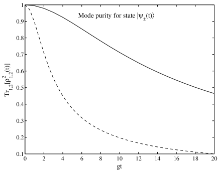
Figure 3: This shows the mode purity as function of the effective interaction time for the field states $|\psi_{\pm}(t)\rangle$, defined in equation (7). The solid curve is the purity for initial squeezed states and the dashed curve when the two modes are prepared in coherent states. For both cases, the average numbers of photons are $\bar{n}=150$ and $\bar{m}=50$ and the squeezing parameters are $r_{1}=r_{2}=1$. For large times the two modes becomes entangled, which is because of the exponent $\exp(\pm igt\sqrt{(m+1)n})$ in the expression for $|\psi_{\pm}(t)\rangle$. The mixing of the modes is greatly reduced for the squeezed states due to the sharp photon distribution.

Even while the two modes in the states $|\psi_{\pm}\rangle$ becomes entangled, it is not necessarily the case for the modes in the actual state of the field. We saw that at the disentanglement times, the field will be in a linear combination of $|\psi_{+}\rangle$ and $|\psi_{-}\rangle$, also if we do a conditional measurement of the atomic state, after a time $t$, the field will be left in a linear combination of the above states. Assume, for example, an atom, initially in the state $|b\rangle$, also being measured in $|b\rangle$ after a time $t$, the field will then be in the state

$$\begin{array}[]{lll}|\psi_{field}(t)\rangle&=&\frac{1}{N}\sum_{n,m}C_{n}C_{m}\cos(gt\sqrt{(m+1)n})|n,m\rangle\\ \\ &=&\frac{1}{2N}\left(|\psi_{+}(t)\rangle+|\psi_{-}(t)\rangle\right),\end{array}$$ (18)

where $N$ is a normalization constant. The mode purity for this state is plotted in figure 4 with $\bar{n}=100$, $\bar{m}=50$ and $r_{1}=r_{2}=1$. At the disentanglement times $gt_{0}^{(j)}$ the purity is greatly increased. At these times, according to equation (14), the state of mode 2 becomes equal in both of the states $|\psi_{\pm}\rangle$ and consequently disentangled from mode 1.

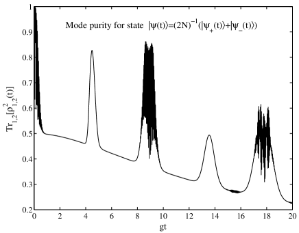
Figure 4: This, as in the previous figure 3, also gives the mode purity, but for the field state $|\psi(t)\rangle=(2N)^{-1}(|\psi_{+}(t)\rangle+|\psi_{-}(t)\rangle)$, where $|\psi_{\pm}(t)\rangle$ are defined in equation (7). Here $N$ is a normalization constant and the two modes are initially in squeezed states (12) with $\bar{n}=100$ and $\bar{m}=50$ and squeezing parameters $r_{1}=r_{2}=1$. The periodic increase of the purity can be understood from equation (14). At these times, either the state of mode one or two, becomes equal in the approximate expressions for the two states $|\psi_{\pm}(t)\rangle$ and consequently disentangle from the other mode.

IV Quantum information processing and entangled states

In this section we show how the Raman-coupled model could be used for quantum logic operations and how various entangled states of the field and atoms can be prepared. In all these examples, except in section IV.3, the fields just contain a few photons and thus, the large field approximations are not used. However, in the section IV.3 on preparation of Schrödinger cat states of the two modes, the large field approximations are very helpful for getting a better understanding of the dynamics.

IV.1 Field mode quantum logic

Let us assume that the effective interaction time is chosen $gt\sqrt{3}=\pi$ and that the two modes are prepared in either of the Fock states $|0\rangle$ or $|3\rangle$. For the atom initially in $|a\rangle$ or $|b\rangle$, the state will, according to equation (4), evolve as

$$\begin{array}[]{lcl}|0,0,a\rangle\rightarrow|0,0,a\rangle&&|0,0,b\rangle\rightarrow|0,0,b\rangle\\ \\ |0,3,a\rangle\rightarrow-|0,3,a\rangle&&|0,3,b\rangle\rightarrow|0,3,b\rangle\\ \\ |3,0,a\rangle\rightarrow|3,0,a\rangle&&|3,0,b\rangle\rightarrow-|3,0,b\rangle\\ \\ |3,3,a\rangle\rightarrow|3,3,a\rangle&&|3,3,b\rangle\rightarrow|3,3,b\rangle.\end{array}$$ (19)

The above transformation describes a quantum phase gate on the two modes, where the atom state acts as an ancilla state. Note that the initial state of the atom decides which field state that changes sign.

IV.2 Atomic quantum logic

Having looked at quantum logic with field modes acting as qubits, we now show how the atom also can be used as an information carrier. Assume mode one to be in either of the Fock states $|0\rangle$ or $|n^{\prime}\rangle$ while mode two is always in vacuum, $|0\rangle$. If the interaction time is such that $gt\sqrt{n^{\prime}}=\pi$, we get for the atomic states $|\phi_{\pm}\rangle=\frac{1}{\sqrt{2}}(|a\rangle\pm|b\rangle)$

$$\begin{array}[]{c}|0,0,\phi_{\pm}\rangle\rightarrow|0,0,\phi_{\pm}\rangle\\ \\ |n^{\prime},0,\phi_{\pm}\rangle\rightarrow|n^{\prime},0,\phi_{\mp}\rangle.\end{array}$$ (20)

Thus, the atomic state is flipped if mode one is in the state $|n^{\prime}\rangle$ while it is unchanged if mode one is in the vacuum. The transformation (20) is identified as a C-NOT quantum logic gate; mode one is the control bit and the atom, the target bit, is flipped depending on the state of the control bit.

IV.3 Entangled Schrödinger cat states

In section III it was shown that when the atom disentangles from the field, in the large photon limit, the state for the modes will be linear combination of the states $|\psi_{\pm}(gt_{0}^{(j)})\rangle$. If the initial state of the atom is $|a\rangle$ or $|b\rangle$ the weight of these field states will be the same. In a first approximation, for coherent field states, the interaction modifies the states by just a phase. If the initial field phases are zero, it means that the interaction will split up the initial state into two parts, one with negative and one with positive phases. For example, an initial state $|\Psi(0)\rangle=|\nu,\mu,a\rangle$ and choosing $\kappa=3$ ($\kappa=\bar{n}/\bar{m}$) will evolve, using the approximation (15), into

$$\begin{array}[]{lll}|\Psi(gt_{0}^{(0)})\rangle&=&\frac{1}{\sqrt{2}}\left(i|a\rangle+|b\rangle\right)\otimes\\ \\ &&\!\!\frac{i}{N}\!\!\left(\!|\nu e^{-i\pi/4}\rangle|\mu e^{-i3\pi/4}\rangle-|\nu e^{i\pi/4}\rangle|\mu e^{i3\pi/4}\rangle\!\right)\!,\end{array}$$ (21)

where, again, $N$ is the normalization constant. Thus, the two field modes in the above expression are both in Schrödinger cat states and they are, at the same time, also maximally entangled with each other. However, for initial coherent states, the two modes in the states $|\psi_{\pm}\rangle$ will become entangled with each other very rapidly, so that the approximation (15) fails for disentanglement times not short enough. From the figure 3 (dashed curve) we note that the purity of the two modes at the first disentanglement time is $P_{mode}\approx 0.60$ for $\bar{n}=150$ and $\bar{m}=50$. So the expression (21) for the state is in fact not a good approximation when $\bar{n}=150$ and $\bar{m}=50$. On the other hand, we saw that the time-scale for mode-mode entanglement was much longer for sub-Poissonian squeezed coherent states. This suggests that by using squeezed coherent initial field states, it is possible to prepare the two modes in entangled Schrödinger cat states. According to figure 3 (solid curve) the corresponding mode purity is $P_{mode}\approx 0.96$, which indicates that the first order approximation (15) is supposed to be acceptable. Figure 5 is a plot of the $Q$-functions, $Q_{1,2}^{\pm}(\alpha,t)=\langle\alpha|\rho_{1,2}^{\pm}(t)|\alpha\rangle$, for the two modes at times $t=0$ and $t=t_{0}^{(1)}$. The initial field states are the same as the ones used for the solid curve in figure 3. The figure 5, together with the purity $P_{mode}\approx 0.96$, clearly shows that the two modes will be in an entangled Schrödinger cat state with the correct estimated phases. Note that this kind of phase-space plot is not enough to give all the information about the state of the two modes, for example, it does not tell us the degree of entanglement between the modes. For long times the large field approximations for the field states will eventually fail, however, they still give an indication of how the separate states behave in phase-space.

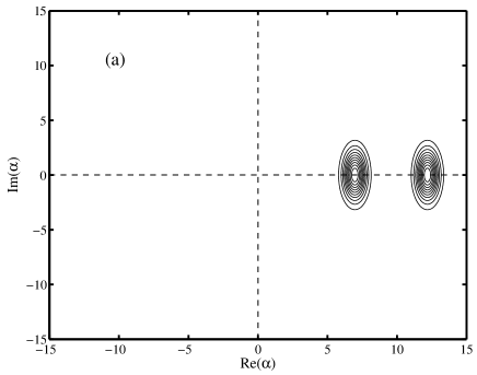
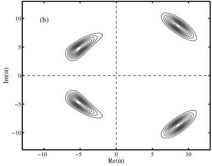
Figure 5: These two contour plots show the various reduced $Q$-functions $Q_{1,2}^{\pm}(\alpha,t)=\langle\alpha|\rho_{1,2}^{\pm}(t)|\alpha\rangle$, at (a) the time zero, and (b) first disentanglement time $gt_{0}^{(1)}$. The two modes are initially in squeezed states with $\bar{n}=150$, $\bar{m}=50$ and $r_{1}=r_{2}=1$, which are seen in (a). In figure 5 (b) it is clear how the two separate modes’ initial states splits up into two parts, characterizing the Schrödinger cats. Note that the phases of the fields agree well with the predicted phases from the approximations, see, for example, equation (21). The shapes of the $Q$-functions for mode two, with lower average number of photons, have changed more during the evolution than for mode one.

IV.4 EPR-states

For $gt=\pi/4$ we get, from equation (4), the following evolution

$$\begin{array}[]{c}|0,1,a\rangle\rightarrow\frac{1}{\sqrt{2}}\left(|0,1,a\rangle-i|1,0,b\rangle\right).\end{array}$$ (22)

If the atom, when it leaves the cavity after a time $gt=\pi/4$, experiences a $\pi/2$-pulse, which means that $|a\rangle\rightarrow\frac{1}{\sqrt{2}}(|a\rangle+|b\rangle)$ and $|b\rangle\rightarrow\frac{1}{\sqrt{2}}(|a\rangle-|b\rangle)$, and then the atomic state is measured in the $\left\{|a\rangle,|b\rangle\right\}$ basis, the two will be in an EPR-state. Depending on the measured atomic state, the two modes are left in the maximally entangled states

$$\begin{array}[]{c}|\mathrm{EPR}\rangle_{-}=\frac{1}{\sqrt{2}}(|0,1\rangle-i|1,0\rangle)\\ \\ |\mathrm{EPR}\rangle_{+}=\frac{1}{\sqrt{2}}(|0,1\rangle+i|1,0\rangle),\end{array}$$ (23)

when the measurement result is $|a\rangle$ and $|b\rangle$ respectively.

IV.5 GHZ-states

Let us assume that the two cavity modes could be prepared in the states $|\pm\rangle=\frac{1}{\sqrt{2}}(|0\rangle\pm|3\rangle)$. We again chose the interaction time so that $gt\sqrt{3}=\pi$ and we see from (19), that after two atoms has passed the cavity, one after the other, the states of the modes will be flipped if the two atomic states were $|a\rangle_{1}|b\rangle_{2}$ or $|b\rangle_{1}|a\rangle_{2}$, while if both atoms where in the same state during the passage, the field is left unchanged. For example

$$|+,+\rangle\!\frac{1}{\sqrt{2}}(|a\rangle_{1}\pm|b\rangle_{1})|a\rangle_{2}\!\rightarrow\!\!\frac{1}{\sqrt{2}}(|+,+,a\rangle_{1}\pm|-,-,b\rangle_{1})|a\rangle_{2},$$ (24)

which means that the interaction leaves the first atom and the two cavity modes in a GHZ-state. Note that the order of the atoms does not matter, so the prepared GHZ-state could equally well include the two modes and the second atom instead.

V Conclusion

In this paper we looked at a theoretical treatment of a three-level Raman system which is coupled to a quantised two-mode cavity. Thus the system has one atom and two modes as sub-systems. An adiabatic elimination of the upper level ensures that when the atom transfers from one lower atomic state to the other, there is a corresponding transfer of photons between the modes. The atom passes through the cavity resulting in a finite interaction time, but during that time we try to effect changes on the quantum states in the cavity. By adjusting the interaction time, one of the three subsystems may disentangle from the others, and can, in such a way, be used to perform a controlled transformation of the remaining two systems.

A key approximation in our model, is concerned with the adiabatic elimination of the upper atomic state, which requires a sufficient two-photon detuning. (For a calculation of what is required, see Ref. wu .) Unfortunately, such a detuning has the effect of reducing the effective two-photon coupling $g$ when compared to the single photon couplings (such as $g_{ab}$). This would slow down the dynamics and make the system more vulnerable to decoherence. However, one advantage of generating entangled Schrödinger cat states in this two-photon model is that it can be done very quickly, i.e. before decoherence becomes too significant. The new feature, compared to the single mode Jaynes-Cummings model, is the appearance of the highly controllable photon number ratio $\kappa$ appearing in the disentanglement time, equation (9).

We have shown how this Raman cavity system can be used as a phase gate with the two field modes carrying qubits and the atom acting as an ancilla state. The state of the atom can be measured after this gate and be used to confirm the correct operation of the phase gate without the destruction of the qubits.

We have also shown how to make a controlled-not gate if the atomic system holds a qubit. Recently many schemes have been proposed for large scale quantum computation on trapped atoms inside a cavity, see atomlogic . The logic gate (20) could be used in such models if external lasers, in a controlled way, are used to Stark-shift the different energy levels for the atoms involved.We have also shown how some interesting entangled states may be produced. In particular, as well as entangled Schrödinger cat states, we can make EPR-type states of the electromagnetic field and a GHZ state of the field modes and an atom. These states and the proposed quantum logic elements may make this an interesting system to pursue experimentally and theoretically in the future.

References

- (1) Nielsen M. A., and Chuang I. L., 2000, Quantum Computing and Quantum Information (Cambridge).
- (2) Jaynes, E. T., and Cummings, F. W., 1963, Proc. IEEE, 51, 89.
- (3) Messina A., Maniscalco S., and Napoli A., 2003, J. Mod. Opt., 50, 1.
- (4) Gea-Banacloche J., 1990, Phys. Rev. Lett., 65, 3385, Gea-Banacloche J., 1991, Phys. Rev. A, 44, 5913.
- (5) Auffeves A., Maioli P., Meunier T., Gleyzes S., Nogues G., Brune M., Raimond J. M., and Haroche S., arXiv:quant-ph/0307185.
- (6) Walls D. F., and Milburn G. J., 1985, Phys. Rev. A, 31, 2403. Phoenix S. J. D., 1990, Phys. Rev. A, 41, 5132.
- (7) Fang M. F., Zhou Q. P., and Zhou P., 1999, Acta Phys. Sin., 8, 401.
- (8) Alexanian M., and Bose S. K., 1995, Phys. Rev. A, 52, 2218.
- (9) Deb B., Gangopadhyay G., and Ray S., 1993, Phys. Rev. A, 48, 1400.
- (10) Rekdal P. K., Skagerstam B. S. K., and Knight P. L., arXiv:quant-ph/0301148.
- (11) Nasreen T., and Zaheer K., 1994, Phys. Rev. A, 49, 616.
- (12) Cardimona D. A., Kovanis V., Sharma M. P., and Gavrielides A., 1991, Phys. Rev. A, 43, 3710.
- (13) Feng M., 2002, Phys. Rev. A, 66, 054303, Pachos J., and Walther H., 2002, Phys. Rev. Lett. 89, 187903-1.
- (14) Wu Y., 1996, Phys. Rev. A, 54, 1586.