Vectorlike representation of one-dimensional scattering

Abstract

We present a self-contained discussion of the use of the transfer-matrix formalism to study one-dimensional scattering. We elaborate on the geometrical interpretation of this transfer matrix as a conformal mapping on the unit disk. By generalizing to the unit disk the idea of turns, introduced by Hamilton to represent rotations on the sphere, we develop a method to represent transfer matrices by hyperbolic turns, which can be composed by a simple parallelogramlike rule.

I Introduction

The quantum mechanics of one-dimensional scattering describes many actual physical phenomena to a good approximation. In consequence, this topic continues as an active line of research with strong implications both in fundamental Pere83 ; Bian94 ; Bian95 ; Chebo96 ; Viss99 ; Miya00 and in more applied aspects, such as the study of tunnelling phenomena in superlattices Tsu73 ; Esak86 ; Haug89 , to cite only a representative example.

Apart from this interest in research, scattering in one dimension is also appealing from a pedagogical point of view and is an important part in the syllabus of any graduate course in quantum mechanics. The advantage of the one-dimensional treatment is that one does not need special mathematical functions, while still retaining sufficient complexity to illustrate physical concepts. It is therefore not surprising that there have been many didactic articles dealing with various aspects of such scattering Eber65 ; Form76 ; Kama84 ; Dijk92 ; Noga96 ; Barl00 ; Barl04 . However, these papers emphasize concepts such as partial-wave decomposition, Lippmann-Schwinger integral equations, the transition operator, or parity-eigenstate representation, paralleling as much as possible their analogous in two and three dimensions. In other words, these approaches, like most if not all the standard textbooks on the subject Gold64 ; Newt66 ; Cohe77 ; Gali90 , employ the formalism of the $S$ matrix.

The elegance and power of the $S$-matrix formulation is beyond doubt. However, it is a “black-box” theory: the system under study (scatterer) is isolated and is tested through asymptotic states. This is well suited for typical experiments in elementary particle physics, but becomes inadequate as soon as one couples the system to other. The most effective technique for studying such one-dimensional systems is the transfer matrix, in which the amplitudes of two fundamental solutions on either side of a potential cell are connected by a matrix $\mathbf{M}$.

The transfer matrix is a useful object that is widely used in the treatment of layered systems, like superlattices Vint91 ; Webe94 ; Spru03 or photonic crystals Joan95 ; Bend96 ; Tsai98 . Optics, of course, is a field in which multilayers are ubiquitous and the transfer-matrix method is well established Brek60 ; Lekn87 ; Yeh88 . An extensive and up-to-date review of the applications of the transfer matrix to many problems in both classical and quantum physics can be found in Ref. Grif01 .

In recent years a number of concepts of geometrical nature have been introduced to gain further insights into the behavior of scattering in one dimension Pere01 ; Yont02 ; Monz02 ; Spru04 . From these analyses it appears advantageous to view the action of a matrix as a bilinear (or Möbius) transformation on the unit disk. A simple way of characterizing these transformations is through the study of the points that they leave invariant. For example, in Euclidean geometry a rotation can be characterized by having only one fixed point, while a translation has no invariant point. In this paper we shall reconsider the fixed points of the bilinear transformation induced by an arbitrary scatterer, showing that they can be classified according to the trace of the transfer matrix has a magnitude lesser than, greater than, or equal to 2. In fact, this trace criterion will allow us to classify the corresponding matrices from a geometrical perspective as rotations, translations or, parallel displacements, respectively, which are the basic isometries (i. e., the transformations that preserve distance) of the unit disk.

As we have stressed, the advantage of transfer matrices lies in the fact that they can be easily composed. Of course, as for any matrix product, this composition is noncommutative. A natural question then arises: how this noncommutativity appears in such a geometrical scenario? An elegant answer involves the notion of Hamilton turns Hami53 ; Bied81 . The turn associated with a rotation of axis $\hat{\mathbf{n}}$ and angle $\vartheta$ is a directed arc of length $\vartheta/2$ on the great circle orthogonal to $\hat{\mathbf{n}}$ on the unit sphere. By means of these objects, the composition of rotations is described through a parallelogramlike law: if these turns are translated on the great circles, until the head of the arc of the first rotation coincides with the tail of the arc of the second one, then the turn between the free tail and the head is associated with the resultant rotation. Hamilton turns are thus analogous for spherical geometry to the sliding vectors in Euclidean geometry. It is unfortunate that this elegant idea of Hamilton is not as widely known as it rightly deserves.

Recently, a generalization of Hamilton turns to the unit disk has been developed Juar82 ; Simo89 ; Barr04 . The purpose of this paper is precisely to show how the use of turns affords an intuitive and visual image of all problems involved in quantum scattering in one dimension, and clearly shows the appearance of hyperbolic geometry in the composition law of transfer matrices. These geometrical methods do not offer any inherent advantage in terms of computational efficiency. Apart from their beauty, their benefit for the students lies in the possibility of gaining insights into the qualitative behavior of scattering amplitudes, which is important in developing a physical feeling for this relevant question.

II Superposition principle and transfer matrix

We consider the quantum scattering in one spatial dimension by a potential $V(x)$. We assume this potential to be real (i. e., nonabsorbing) but otherwise arbitrary in a finite interval $(a,b)$, and outside this interval, it is taken to be a constant that we can define to be the zero of energy. We recall that, because $E>0$, the spectrum is continuum and we have two linearly independent solutions for a given value of $E$. In consequence, the general solution of the time-independent Schödinger equation for this problem can be expressed as a superposition of the right-mover $e^{+ikx}$ and the left-mover $e^{-ikx}$:

$$\psi(x)=\left\{\begin{array}[]{ll}A_{+}e^{+ik(x-a)}+A_{-}e^{-ik(x-a)}&x<a,\\ &\\ \psi_{ab}(x)&a<x<b\\ &\\ B_{+}e^{+ik(x-b)}+B_{-}e^{-ik(x-b)}&x>b,\\ \end{array}\right.,$$ (1)

where $k^{2}=2mE/\hbar^{2}$ and the subscripts $+$ and $-$ indicate that the waves propagate to the right and to the left, respectively (see Fig. 1). The origins of the movers have been chosen so as to simplify as much as possible subsequent calculations.

To complete in a closed form the problem one must solve the Schrödinger equation in $(a,b)$ to obtain $\psi_{ab}$ and then invoke the appropriate boundary conditions, involving not only the continuity of $\psi(x)$, but also of its derivative. In this way, one obtains two linear relations among the coefficients $A_{\pm}$ and $B_{\pm}$, which can be solved for any two amplitudes in terms of the other two, and the result can be expressed as a matrix equation. The usual choice in most textbooks is to write the outgoing amplitudes in terms of the incoming amplitudes (which are the magnitudes one can externally control) using the so-called scattering matrix $\mathbf{S}$. For our purposes in this paper, it will prove crucial to express a linear relation between the wave amplitudes on both sides of the scatterer, namely,

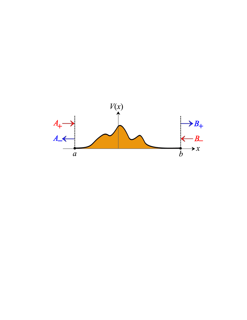
Figure 1: Illustration of the scattering from an arbitrary potential, showing the input ($A_{+}$ and $B_{-}$) and output ($A_{-}$ and $B_{+}$) amplitudes.

$$\left(\begin{array}[]{c}A_{+}\\ A_{-}\end{array}\right)=\mathbf{M}\left(\begin{array}[]{c}B_{+}\\ B_{-}\end{array}\right),$$ (2)

where $\mathbf{M}$ is the transfer matrix. Obviously, the complete determination of the $\mathbf{M}$ amounts to solving the Schrödinger equation and, in consequence, it is not, in general, a simple exercise. Nevertheless, some properties of the transfer matrix are universal Grif01 . First, we note that time-reversal invariance implies [because $V(x)$ is real] that $\psi^{\ast}(x)$ is also a solution. Since this symmetry interchanges incoming and outgoing waves this means that

$$\left(\begin{array}[]{c}A_{-}^{\ast}\\ A_{+}^{\ast}\end{array}\right)=\mathbf{M}\left(\begin{array}[]{c}B_{-}^{\ast}\\ B_{+}^{\ast}\end{array}\right).$$ (3)

Comparing with Eq. (2) leads to the conclusion that the matrix $\mathbf{M}$ must be of the form

$$\mathbf{M}=\left(\begin{array}[]{cc}\alpha&\beta\\ \beta^{\ast}&\alpha^{\ast}\end{array}\right).$$ (4)

Next we assess the implications of the conservation of probability. Since the probability current is

$$J=-i\frac{\hbar}{2m}\left(\psi^{\ast}\frac{d\psi}{dx}-\psi\frac{d\psi^{\ast}}{dx}\right),$$ (5)

the continuity equation entails

$$|A_{+}|^{2}-|A_{-}|^{2}=|B_{+}|^{2}-|B_{-}|^{2},$$ (6)

which is tantamount to

$$\det\mathbf{M}=1.$$ (7)

The set of $2\times 2$ complex matrices of the form (4) satisfying the constraint (7) constitute a group called SU(1, 1) Wybo74 .

If we take an incident wave from the left ($B_{-}=0$) and fix $A_{+}=1$, then

$$\left(\begin{array}[]{c}1\\ r\end{array}\right)=\mathbf{M}\left(\begin{array}[]{c}t\\ 0\end{array}\right),$$ (8)

where the complex numbers $r$ and $t$ are the corresponding reflection and transmission amplitudes. This determines the first column of $\mathbf{M}$. Denoting the corresponding amplitudes for waves incident from the right as $r^{\prime}$ and $t^{\prime}$ and repeating the procedure, one easily finds that time-reversal invariance imposes

$$t^{\prime}=t,$$

(9)

$$\displaystyle\frac{r^{\prime}}{t^{\prime}}=-\frac{r^{\ast}}{t^{\ast}},$$

while conservation of the flux determines

$$|r|^{2}+|t|^{2}=1.\\$$

The final form of our transfer matrix is then

$$\mathbf{M}=\left(\begin{array}[]{cc}1/t&r^{\ast}/t^{\ast}\\ r/t&1/t^{\ast}\end{array}\right).$$ (10)

In the particular case of a symmetric potential it is obvious that $r=r^{\prime}$ and therefore the matrix element $\beta$ is an imaginary number.

For later use, we will now bring up the paradigmatic example of a rectangular potential barrier of width $L$ and height $V_{0}$. Since the calculations can be easily carried out, we skip the details and merely quote the results for $r$ and $t$:

$$r = e^{+ikL}\left[\frac{(k^{2}+\kappa^{2})\sinh(\kappa L)}{(k^{2}-\kappa^{2})\sinh(\kappa L)+2ik\kappa\cosh(\kappa L)}\right],$$

$$t = e^{-ikL}\left[\frac{2ik\kappa}{(k^{2}-\kappa^{2})\sinh(\kappa L)+2ik\kappa\cosh(\kappa L)}\right],$$

where $k^{2}=2mE/\hbar^{2}$ and $\kappa^{2}=2m(E-V_{0})/\hbar^{2}$. These coefficients correspond to the case $E<V_{0}$. When $E>V_{0}$ the above expressions remain valid with the formal substitution $\kappa\rightarrow i\bar{\kappa}$. Finally, when $E=V_{0}$, a limiting procedure gives

$$r = e^{+ikL}\left[\frac{1}{1+2i/(kL)}\right]\,,$$

$$t = e^{-ikL}\left[\frac{1}{1+kL/(2i)}\right]\,.$$

Be aware that the transfer matrix depends on the choice of basis vectors. For example, instead of specifying the amplitudes of the right and left-moving waves, we could write a linear relation between the values of the wave function and its derivative at two different points Spru93 :

$$\left(\begin{array}[]{c}\psi(a)\\ \psi^{\prime}(a)\end{array}\right)=\bm{\mathcal{M}}\left(\begin{array}[]{c}\psi(b)\\ \psi^{\prime}(b)\end{array}\right).$$ (13)

These two basis vectors are related by

$$\left(\begin{array}[]{c}\psi(a)\\ \psi^{\prime}(a)\end{array}\right)=\bm{\mathcal{U}}\left(\begin{array}[]{c}A_{+}\\ A_{-}\end{array}\right),$$ (14)

where

$$\bm{\mathcal{U}}=\left(\begin{array}[]{cc}1&1\\ ik&-ik\end{array}\right),$$ (15)

and analogously at the point $b$. Correspondingly, the matrix $\mathbf{M}$ in this representation is

$$\bm{\mathcal{M}}=\bm{\mathcal{U}}\mathbf{M}\bm{\mathcal{U}}^{-1}=\left(\begin{array}[]{cc}\mathfrak{a}&\mathfrak{b}\\ \mathfrak{c}&\mathfrak{d}\end{array}\right),$$ (16)

where

$$\mathfrak{a}=\mathrm{Re}\,\alpha+\mathrm{Re}\,\beta,\qquad\displaystyle\mathfrak{b}=\frac{1}{k}(\mathrm{Im}\,\alpha-\mathrm{Im}\,\beta),$$

(17)

$$\mathfrak{c}=-k(\mathrm{Im}\,\alpha+\mathrm{Im}\,\beta)\,,\qquad\mathfrak{d}=\mathrm{Re}\,\alpha-\mathrm{Re}\,\beta\,.$$

Since the trace and the determinant are preserved by this matrix conjugation, we have that $\det\bm{\mathcal{M}}=+1$. In consequence, in this representation transfer matrices belong to the group SL(2, $\mathbb{R}$) of unimodular $2\times 2$ matrices with real elements.

Transfer matrices are very convenient mathematical objects. Suppose we know how the wave functions “propagate” from point $b$ to point $a$, with a transfer matrix we symbolically write as $\mathbf{M}(a,b)$, and also from $c$ to $b$, with $\mathbf{M}(b,c)$. The essential point is that propagation from $c$ to $a$ is then described by the product of transfer matrices:

$$\mathbf{M}(a,c)=\mathbf{M}(a,b)\,\mathbf{M}(b,c).$$ (18)

The multiplicative property is rather useful: we can connect simple scatterers as building blocks to create an intricate potential landscape and determine its transfer matrix by simple multiplication. The usual scattering matrix does not have this important property because the incoming amplitudes for the overall system cannot be obtained in terms of the incoming amplitudes for every subsystem.

III Understanding scattering amplitudes in the unit disk

We observe that because of the flux conservation in Eq. (6), the complex quotients

$$z_{a}=\frac{A_{-}}{A_{+}}\,,\qquad z_{b}=\frac{B_{-}}{B_{+}}\,,$$ (19)

contain the essential information about the wave function and omit a global phase factor. The action of a transfer matrix can be then seen as a mapping from the value on $z_{b}$ to the value on $z_{a}$ according to

$$z_{a}=\Phi[\mathsf{M},z_{b}]=\frac{\beta^{\ast}+\alpha^{\ast}z_{b}}{\alpha+\beta z_{b}}\ ,$$ (20)

which can be appropriately called the scattering transfer function Monz02 . The action (20) is known as a bilinear or Möbius mapping and is a conformal mapping of the entire plane onto itself and which maps circles into circles.

Properties of this mapping are part of any course in complex variables and have been discussed, in the context of a relativisticlike presentation of multilayer optics, in Refs. Yont02  and Monz02 . One can check that points in the unit disk are mapped onto points in the unit disk, while the unit circle maps into itself. The external region remains also invariant. For the usual scattering solution with incident waves from the left ($B_{-}=0$), we have $z_{b}=0$ and $z_{a}=r$. Conversely, when $z_{a}=0$, we have the necessary and sufficient condition for a transparent potential. Note that the unit circle represents the action of a system with $|r|=1$, that is, of a perfect “mirror”.

To classify the scatterer action it proves convenient to work out the fixed points of the mapping Ande99 ; that is, the wave configurations such that $z_{a}=z_{b}\equiv z_{f}$ in Eq. (20):

$$z_{f}=\Phi[\mathbf{M},z_{f}],$$ (21)

whose solutions are

$$z_{f\pm}=\frac{1}{2\beta}\left\{-2i\ \mathrm{Im}(\alpha)\pm\sqrt{[\mathop{\mathrm{Tr}}\nolimits(\mathbf{M})]^{2}-4}\right\}.$$ (22)

When $[\mathop{\mathrm{Tr}}\nolimits(\mathbf{M})]^{2}<4$ the action is said elliptic and has only one fixed point inside the unit disk. Since in the Euclidean geometry a rotation is characterized for having only one invariant point, this action can be appropriately called a hyperbolic rotation.

When $[\mathop{\mathrm{Tr}}\nolimits(\mathbf{M})]^{2}>4$ the action is said hyperbolic and has two fixed points, both on the unit circle. The geodesic line joining these two fixed points remains invariant and thus, by analogy with the Euclidean case, this action will be called a hyperbolic translation.

Finally, when $[\mathop{\mathrm{Tr}}\nolimits(\mathbf{M})]^{2}=4$ the system action is parabolic and has only one (double) fixed point on the unit circle.

It is worth mentioning that, for the example of the rectangular barrier discussed previously, one can use Eqs. (II) and (II) to check that its action becomes elliptic, hyperbolic, or parabolic according to $E$ is greater than, lesser than, or equal to $V_{0}$, respectively.

To proceed further let us note that by taking the conjugate of $\mathbf{M}$ with any matrix $\mathbf{C}\in$ SU(1, 1), i. e.,

$$\mathbf{M}_{\mathrm{C}}=\mathbf{C}\ \mathbf{M}\ \mathbf{C}^{-1},$$ (23)

we obtain another matrix of the same type, since $\mathop{\mathrm{Tr}}\nolimits(\mathbf{M})=\mathop{\mathrm{Tr}}\nolimits(\mathbf{M}_{\mathrm{C}})$. Conversely, if two systems have the same trace, one can always find a matrix $\mathbf{C}$ satisfying Eq. (23).

The fixed points of $\mathbf{M}_{\mathrm{C}}$ are then the image by $\mathbf{C}$ of the fixed points of $\mathbf{M}$. In consequence, given any transfer matrix $\mathbf{M}$ we can always reduce it to one of the following canonical forms Sanc01 :

$$\mathbf{K}_{\mathrm{C}}(\theta) = \left(\begin{array}[]{cc}\exp(i\theta/2)&0\\ 0&\exp(-i\theta/2)\end{array}\right)\,,$$ (26)

$$\mathbf{A}_{\mathrm{C}}(\xi) = \left(\begin{array}[]{cc}\cosh(\xi/2)&i\,\sinh(\xi/2)\\ -i\,\sinh(\xi/2)&\cosh(\xi/2)\end{array}\right)\ ,$$ (29)

$$\mathbf{N}_{\mathrm{C}}(\nu) = \left(\begin{array}[]{cc}1-i\nu/2&\nu/2\\ \nu/2&1+i\nu/2\end{array}\right)\,,$$ (32)

which have as fixed points the origin (elliptic), $+i$ and $-i$ (hyperbolic) and $+i$ (parabolic), respectively.

For the canonical forms (26) the corresponding bilinear transformations are

$$z^{\prime} = \Phi[\mathbf{K}_{\mathrm{C}}(\theta),z]=z\exp(-i\theta)\ ,$$

$$z^{\prime} = \Phi[\mathbf{A}_{\mathrm{C}}(\xi),z]=\frac{z-i\tanh(\xi/2)}{1+iz\tanh(\xi/2)}\,,$$ (33)

$$z^{\prime} = \Phi[\mathbf{N}_{\mathrm{C}}(\nu),z]=\frac{z+(1+iz)\nu/2}{1+(z-i)\nu/2}\,.$$

In words, given a generic point $z$ in the unit disk, and varying the parameters $\theta$, $\xi$, or $\nu$ in Eq. (III), the transformed points $z^{\prime}$ describe a characteristic curve that we shall call the orbit associated to $z$ by the transformation. In Fig. 1.a we have plotted some orbits for different values of $z$ for each one of these canonical forms. For matrices $\mathbf{K}_{\mathrm{C}}(\theta)$ the orbits are circumferences centered at the origin. For the matrices $\mathbf{A}_{\mathrm{C}}(\xi)$, they are arcs of circumference going from the point $+i$ to the point $-i$ through $z$. Finally, for the matrices $\mathbf{N}_{\mathrm{C}}(\nu)$ the orbits are circumferences passing through the points $i$, $z$, and $-z^{\ast}$. Note that this is in full agreement with the geometrical meaning of these transformations. In Fig. 1.b we have plotted the corresponding orbits for arbitrary fixed points, obtained by conjugation of the previous ones. The explicit construction of the family of matrices $\mathbf{C}$ is not difficult: it suffices to impose that $\mathbf{C}$ transforms the fixed points of $\mathbf{M}$ into the ones of $\mathbf{K}_{\mathrm{C}}(\theta)$, $\mathbf{A}_{\mathrm{C}}(\xi)$, or $\mathbf{N}_{\mathrm{C}}(\nu)$, respectively.

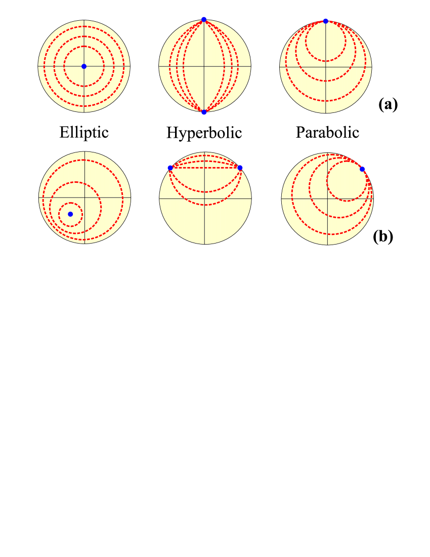
Figure 2: Plot of typical orbits in the unit disk: (a) canonical transfer matrices as given in Eq. (26) and (b) arbitrary transfer matrices obtained by conjugation as in Eq. (23) of the previous ones.

IV Application: geometrical representation of finite periodic systems

As an important application of the previous formalism, let us suppose that we repeat $N$ times our system represented by $\mathbf{M}$. This is called a finite periodic system and, given its relevance, has been extensively discussed in the literature Vezz86 ; Kalo91 ; Griff92 ; Rozm94 ; Chup94 ; Livi94 ; Erdo97 ; Barr99 . Obviously, the overall transfer matrix is now $\mathbf{M}^{N}$, so all the algebraic task reduces to the obtention of a closed expression for the $N$th power of the matrix $\mathbf{M}$. Although there are several elegant ways of computing this, we shall instead apply our geometrical picture. To this end we represent the transformed state by the $N$-period structure by the point

$$z_{N}=\Phi[\mathbf{M},z_{N-1}]=\Phi[\mathbf{M}^{N},z_{0}],$$ (34)

where $z_{0}$ denotes here the initial point.

Henceforth, we shall take $z_{0}=0$, which is not a serious restriction as it corresponds to the case in which no wave incides from the right. Note also that all the points $z_{N}$ lie in the orbit associated to the initial point $z_{0}$ by the basic period, which is determined by its fixed points: the character of these fixed points determine thus the behavior of the periodic structure.

To illustrate how this geometrical approach works in practice, in Fig. 3 we have plotted the sequence of successive iterates obtained numerically for different kind of transfer matrices according to our previous classification.

In the elliptic case, the points $z_{N}$ revolve in the orbit centered at the fixed point and the system never reaches the unit circle. On the contrary, for the hyperbolic and parabolic cases the iterates converge to one of the fixed points on the unit circle, although with different laws. Since the unit circle represents a perfect “mirror”, this means that strong reflection occurs and we are in a forbidden band. In other words, in this geometrical picture the route to a forbidden band can be understood as the convergence of the point representing the action of the system to the unit circle.

Obviously, this is in perfect agreement with the standard treatment, which gets these band gaps from an eigenvalue equation for the Bloch factor in an infinite periodic structure: since the Bloch phase is $|\mathop{\mathrm{Tr}}\nolimits(\mathbf{M})|$, and strong reflection occurs when this trace exceeds 2 in magnitude (the band edge is located precisely when the trace equals 2) Barr03 .

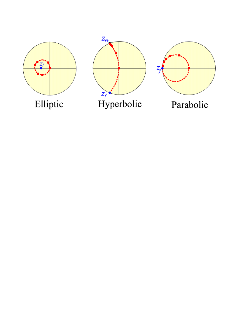
Figure 3: Plot of the successive iterates ($N=1,\ldots,5$) for an elliptic, hyperbolic, and parabolic action starting from the origin as the initial point. Only hyperbolic and parabolic actions tend to the unit circle.

Let us focus then on the hyperbolic case, which, in this approach, corresponds to a translation in the unit disk. We can explicitly compute the $N$th iterate for the canonical form $\mathbf{A}_{\mathrm{C}}$, since $\mathbf{A}_{\mathrm{C}}(\xi_{1})\mathbf{A}_{\mathrm{C}}(\xi_{2})=\mathbf{A}_{\mathrm{C}}(\xi_{1}+\xi_{2})$ [this property holds true for all the canonical forms in Eq. (26)]. Finally, it suffices to conjugate as in (23) to obtain, after some calculations, that

$$z_{N}=\frac{1-\chi^{N}}{1-\chi^{N}(z_{f+}/z_{f-})}z_{f+},$$ (35)

where

$$\chi=\frac{\alpha+\beta z_{f-}}{\alpha+\beta z_{f+}}$$ (36)

is a complex number satisfying $|\chi|<1$. Here $z_{f\pm}$ are the fixed points of the matrix. Note that, because $z_{0}=0$, this initial point is transformed by the single period into the point $r$. Therefore, $z_{N}$ represents the reflection amplitude of the overall periodic structure, which is obviously different from $r^{N}$. One gets

$$|z_{N}|^{2}=\frac{|\beta|^{2}}{|\beta|^{2}+[\sinh(\xi)/\sinh(N\xi)]^{2}},$$ (37)

where we have denoted

$$\mathrm{Re}\,\alpha=\frac{1}{2}\mathop{\mathrm{Tr}}\nolimits(\mathbf{M})=\cosh(\xi).$$ (38)

Note that $|z_{N}|^{2}$ approaches the unit circle exponentially with $N$, as one could expect from a band stop.

Analogously, for the parabolic case we have

$$z_{N}=\frac{N\beta z_{f}^{2}}{N\beta z_{f}-1},$$ (39)

where $z_{f}$ is the (double) fixed point. One then obtains

$$|z_{N}|^{2}=\frac{|\beta|^{2}}{|\beta|^{2}+(1/N)^{2}},$$ (40)

that goes to unity with a typical behavior $O(N^{-2})$. This is universal in the physics of reflection, as put forward in a different framework by Lekner Lekn87 and Yeh Yeh88 .

V Transfer-matrix composition as a hyperbolic-turn sum

To clarify the geometrical picture of the composition of two scattering systems we briefly recall that the (hyperbolic) metric in the unit disk is defined by Ande99

$$ds^{2}=\frac{dz^{2}}{(1-|z|^{2})^{2}}.$$ (41)

With this metric, it is a simple exercise to work out that the geodesic (path of minimum distance) between two points is the Euclidean arc of the circle through those points and orthogonal to the unit circle. The diameters are also geodesic lines.

The hyperbolic distance between two points $z_{b}$ and $z_{a}$ can be computed from (41) and is

$$d_{\mathbb{H}}(z_{b},z_{a})=\ln\left(\frac{|z_{b}^{\ast}z_{a}-1|+|z_{b}-z_{a}|}{|z_{b}^{\ast}z_{a}-1|-|z_{b}-z_{a}|}\right)\,.$$ (42)

Note that the visual import of the disk with this metric is that a pair of points with a given distance between them will appear to be closer and closer together as their location approaches the boundary circle. Or, equivalently, a pair of points near the boundary of the disk are actually farther apart (via the metric) than a pair near the center of the disk which appear to be the same distance apart.

When these points $z_{b}$ and $z_{a}$ are related by $\mathbf{M}$, the distance between them can be compactly expressed as

$$\zeta=2\ln\left(\frac{1}{2}\{\mathop{\mathrm{Tr}}\nolimits(\mathbf{M})+\sqrt{[\mathop{\mathrm{Tr}}\nolimits(\mathbf{M})]^{2}-4}\}\right)\,.$$ (43)

Let us focus on the case of $[\mathop{\mathrm{Tr}}\nolimits(\mathbf{M})]^{2}>4$. This is not a serious restriction, since it is known that any matrix of SU(1, 1) can be written (in many ways) as the product of two hyperbolic translations Simo89b . The axis of the hyperbolic translation is the geodesic line joining the two fixed points.

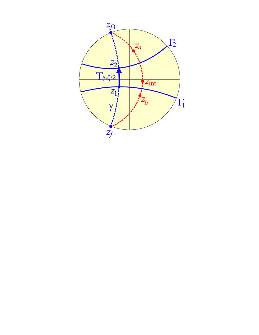
Figure 4: Representation of the sliding turn $\mathbb{T}_{\gamma,\zeta/2}$ in terms of two reflections in two lines $\Gamma_{1}$ and $\Gamma_{2}$ orthogonal to the axis of the translation $\gamma$, which has two fixed points $z_{f+}$ and $z_{f-}$. The transformation of a typical off axis point $z_{b}$ is also shown.

In Euclidean geometry, a translation of magnitude $\zeta$ along a line $\gamma$ can be seen as the product of two reflections in any two straight lines orthogonal to $\gamma$, separated a distance $\zeta/2$. This idea can be translated much in the same way to the unit disk, once the concepts of line and distance are understood in the hyperbolic sense. In consequence, any pair of points $z_{1}$ and $z_{2}$ on the axis of the translation $\gamma$ at a distance $\zeta/2$ can be chosen as intersections of $\Gamma_{1}$ and $\Gamma_{2}$ (orthogonal lines to $\gamma$) with $\gamma$. It is then natural to associate to the translation an oriented segment of length $\zeta/2$ on $\gamma$, but otherwise free to slide on $\gamma$ (see Fig. 4). This is analogous to Hamilton’s turns, and will be called a hyperbolic turn $\mathbb{T}_{\gamma,\zeta/2}$.

Note that using this construction, an off-axis point such as $z_{b}$ will be mapped by these two reflections (through an intermediate point $z_{\mathrm{int}}$) to another point $z_{a}$ along a curve equidistant to the axis. These other curves, unlike the axis of translation, are not hyperbolic lines. The essential point is that once the turn is known, the transformation of every point in the unit disk is automatically established.

Alternatively Barr04 , we can formulate the concept of turn as the “square root” of a transfer matrix: if $\mathbf{M}$ is a hyperbolic translation with $\mathop{\mathrm{Tr}}\nolimits(\mathbf{M})$ positive (equivalently, $\mathrm{Re}(\alpha)>1$), then one can ensure that its square root exists and reads as

$$\sqrt{\mathbf{M}}=\frac{1}{\sqrt{2[\mathrm{Re}(\alpha)+1]}}\left[\begin{array}[]{cc}\alpha+1&\beta\\ \beta^{\ast}&\alpha^{\ast}+1\end{array}\right].$$ (44)

We can easily check that this matrix has the same fixed points as $\mathbf{M}$, but the translated distance is just half the induced by $\mathbf{M}$; that is

$$\zeta_{\mathbf{M}}=2\zeta_{\sqrt{\mathbf{M}}}.$$ (45)

This suggests that the matrix $\sqrt{\mathbf{M}}$ can be appropriately associated to the turn $\mathbb{T}_{\gamma,\zeta/2}$ that represents the translation induced by $\mathbf{M}$.

One may be tempted to extend the Euclidean composition of concurrent vectors to the problem of hyperbolic turns. Indeed, this can be done quite straightforwardly Juar82 . Let us consider the case of the composition of two of these systems represented by matrices $\mathbf{M}_{1}$ and $\mathbf{M}_{2}$ with scattering amplitudes $(r_{1},t_{1})$ and $(r_{2},t_{2})$, in agreement with Eq. (10). The action of the compound system can be expressed as

$$\mathbf{M}_{12}=\mathbf{M}_{1}\mathbf{M}_{2}\,,$$ (46)

and the reflection and transmission amplitudes associated to $\mathbf{M}_{12}$ are

$$r_{12} = \frac{r_{1}+r_{2}\exp(i2\varphi_{1})}{1+r_{1}^{\ast}r_{2}\exp(i2\varphi_{1})},$$

$$t_{12} = \frac{t_{1}t_{2}}{1+r_{1}^{\ast}r_{2}\exp(i2\varphi_{1})},$$

where $t_{1}=|t_{1}|\exp(i\varphi_{1})$.

Let $\zeta_{1}$ and $\zeta_{2}$ be the corresponding translated distances along intersecting axes $\gamma_{1}$ and $\gamma_{2}$, respectively. Take now the associated turns $\mathbb{T}_{\gamma_{1},\zeta_{1}/2}$ and $\mathbb{T}_{\gamma_{2},\zeta_{2}/2}$ and slide them along $\gamma_{1}$ and $\gamma_{2}$ until they are “head to tail”. Afterwards, the turn determined by the free tail and head is the turn associated to the resultant, which represents thus a translation of parameter $\zeta_{12}$ along the line $\gamma_{12}$.

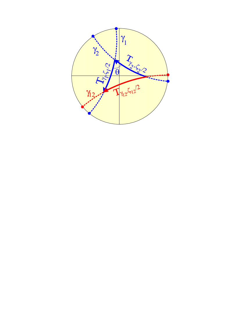
Figure 5: Composition of two scattering systems represented by the hyperbolic turns $\mathbb{T}_{\gamma_{1},\zeta_{1}/2}$ and $\mathbb{T}_{\gamma_{2},\zeta_{2}/2}$. The action of the overall system is obtained by using a parallelogramlike law.

This construction is shown in Fig. 5, where the pertinent parameters are $(r_{1}=-0.9521-i0.0882,t_{1}=0.2532-i0.1468)$ and $(r_{2}=-0.3307-i0.52903,t_{2}=0.6284-i0.4647)$. The application of (V) gives $(r_{12}=0.3736+i0.2014,t_{12}=0.8971-i0.1228)$. The noncommutative character is evident, and can also be inferred from the obvious fact that $\mathbf{M}_{12}\neq\mathbf{M}_{21}$.

In Euclidean geometry, the resultant of this parallelogram law can be quantitatively determined by a direct application of the cosine theorem. For any hyperbolic triangle with sides of lengths $\zeta_{1}$ and $\zeta_{2}$ that make an angle $\theta$, we take the expression from any standard book on hyperbolic geometry Ande99

$$\cosh\zeta_{12}=\cosh\zeta_{1}\cosh\zeta_{2}+\sinh\zeta_{1}\sinh\zeta_{2}\cos\theta,$$ (48)

where $\theta$ is the angle between both sides.

VI Concluding remarks

In summary, what we hope to have accomplished is to present in a clear way the advantages of using the transfer matrix to study one-dimensional scattering. In spite of the slight “cross-talk” between different fields, the transfer matrix is a powerful tool that relies only on linearity of a nonabsorbing system with two input and two output channels. For this reason, it is becoming more and more important in a variety of applications.

We have interpreted the action of a transfer matrix on a wave function as a conformal mapping on the unit disk and we have characterized the basic geometrical actions in terms of its trace. By generalizing to the unit disk Hamilton’s idea of turns, we have provided a remarkably vivid pictorial description of the scattering action, with a composition law that parallels the corresponding one for sliding vectors in Euclidean geometry.

To conclude, we expect that the geometrical scenario presented here could provide an appropriate tool for analyzing the performance of one-dimensional potentials in an elegant and concise way.

References

- (1) A. Peres, “Transfer matrices for one-dimensional potentials,” J. Math. Phys. 24, 1110-1119 (1983).
- (2) M. Sassoli de Bianchi, “Levinson s theorem, zero-energy resonances, and time delay in one-dimensional scattering systems,” J. Math. Phys. 35, 2719-2733 (1994).
- (3) M. Sassoli de Bianchi and M. Di Ventra, “On the number of states bound by one-dimensional finite periodic potentials,” J. Math. Phys. 36, 1753-1764 (1995).
- (4) L. V. Chebotarev and A. Tchebotareva, “Flat resonances in one-dimensional quantum scattering,” J. Phys. A 29, 7259-7277 (1996).
- (5) M. Visser, “Some general bounds for one-dimensional scattering,” Phys. Rev. A 59, 427-438 (1999).
- (6) T. Miyazawa, “Generalized low-energy expansion formula for Green s function of the Fokker-Planck equation,” J. Phys. A 33, 191-225 (2000).
- (7) R. Tsu and L. Esaki, “Tunneling in a finite superlattice,” Appl. Phys. Lett. 22, 562-564 (1973).
- (8) L. Esaki, “A birds-eye-view on the evolution of semiconductor superlattices and quantum wells,” IEEE J. Quantum Electron. QE-22, 1611-1624 (1986).
- (9) E. H. Hauge and J. A. Støvneng, “Tunneling times: a critical review,” Rev. Mod. Phys. 61, 917-936 (1989).
- (10) J. H. Eberly, “Quantum scattering theory in one dimension,” Am. J. Phys. 33, 771-773 (1965).
- (11) J. Formánek, “On phase shift analysis of one-dimensional scattering,” Am. J. Phys. 44, 778-779 (1976).
- (12) A. N. Kamal, “On the scattering theory in one dimension,” Am. J. Phys. 52, 46-49 (1984).
- (13) W. van Dijk and K. A. Kiers, “Time delay in simple one-dimensional systems,” Am. J. Phys. 60, 520-527 (1992).
- (14) Y. Nogami and C. K. Ross, “Scattering from a nonsymmetric potential in one dimension as a coupled-channel problem,” Am. J. Phys. 64, 923-928 (1996).
- (15) V. E. Barlette, M. M. Leite, and S. K. Adhikari, “Quantum scattering in one dimension,” Eur. J. Phys. 21, 435-440 (2000).
- (16) V. E. Barlette, M. M. Leite, and S. K. Adhikari, “Integral equations of scattering in one dimension,” Am. J. Phys. 69, 1010-1013 (2004).
- (17) M. L. Goldberger and K. M. Watson, Collision theory (Wiley, New York, 1964).
- (18) R. G. Newton, Scattering Theory of Waves and Particles (McGraw-Hill, New York, 1966).
- (19) C. Cohen-Tannoudji, B. Diu, and F. Laloë, Quantum Mechanics (Wiley, New York, 1977) Vol. 1.
- (20) A. Galindo and P. Pascual, Quantum Mechanics (Springer-Verlag, Berlin, 1990) Vol. 1.
- (21) B. Vinter and C. Weisbuch, Quantum Semiconductor Structures (Academic, New York, 1991)
- (22) T. A. Weber, “Bound states with no classical turning points in semiconductor heterostructures,” Solid State Comm. 90, 713-716 (1994).
- (23) D. W. L. Sprung, J. D. Sigetich, P. Jagiello, and J. Martorell, “Continuum bound states as surface states of a finite periodic system,” Phys. Rev. B 67, 085318 (2003).
- (24) J. D. Joannopoulos, R. D. Meade, and J. N. Winn, Photonic Crystals (University of Princeton Press, Princeton, N. J., 1995).
- (25) J. M. Bendickson, J. P. Dowling, and M. Scalora, “Analytic expressions for the electromagnetic mode density in finite, one-dimensional, photonic band-gap structures,” Phys. Rev. E 53, 4107-4121 (1996).
- (26) Y. C. Tsai, K. W. Shung, and S. C. Gou, “Impurity modes in one-dimensional photonic crystals: analytic approach,” J. Mod. Opt. 45, 2147-2158 (1998).
- (27) L. M. Brekovskikh, Waves in Layered Media (Academic, New York, 1960).
- (28) J. Lekner, Theory of Reflection (Kluwer, Dordrecht, 1987).
- (29) P. Yeh, Optical Waves in Layered Media (Wiley, New York, 1988).
- (30) D. J. Griffiths and C. A. Steinke, “Waves in locally periodic media,” Am. J. Phys. 69, 137-154 (2001).
- (31) R. Pérez-Álvarez, C. Trallero-Herrero and F. García-Moliner, “1D transfer matrices,” Eur. J. Phys. 22, 275-286 (2001).
- (32) T. Yonte, J. J. Monzón, L. L. Sánchez-Soto, J. F. Cariñena, and C. López-Lacasta, “Understanding multilayers from a geometrical viewpoint,” J. Opt. Soc. Am. A 19, 603-609 (2002).
- (33) J. J. Monzón, T. Yonte, L. L. Sánchez-Soto, and J. F. Cariñena, “Geometrical setting for the classification of multilayers,” J. Opt. Soc. Am. A 19, 985-991 (2002).
- (34) D. W. L. Sprung, G. V. Morozov, and J. Martorell, “Geometrical approach to scattering in one dimension,” J. Phys. A 37, 1861-1880 (2004).
- (35) W. R. Hamilton, Lectures on Quaternions (Hodges & Smith, Dublin, 1853).
- (36) L. C. Biedenharn and J. D. Louck, Angular Momentum in Quantum Physics (Addison, Reading, MA ,1981).
- (37) M. Juárez and M. Santander, “Turns for the Lorentz group,” J. Phys. A 15, 3411-3424 (1982).
- (38) R. Simon, N. Mukunda, and E. C. G. Sudarshan, “Hamilton’s Theory of Turns Generalized to Sp(2,R),” Phys. Rev. Lett. 62, 1331-1334 (1989).
- (39) A. G. Barriuso, J. J. Monzón, L. L. Sánchez-Soto, and J. F. Cariñena, “Vectorlike representation of multilayers,” J. Opt. Soc. Am. A 21, (2004).
- (40) B. G. Wybourne, Classical Groups for Physicists (Wiley, New York, 1974).
- (41) D. W. L. Sprung, H. Wu, and J. Martorell, “Scattering by a finite periodic potential,” Am. J. Phys. 61, 1118-1124 (1993).
- (42) J. W. Anderson, Hyperbolic geometry (Springer Undergraduate Series) (Springer, New York, 1999)
- (43) L. L. Sánchez-Soto, J. J. Monzón, T. Yonte, and J. F. Cariñena, “Simple trace criterion for classification of multilayers,” Opt. Lett. 26, 1400-1402 (2001).
- (44) D. J. Vezzetti and M. Cahay, “Transmission resonances in finited repeated structures,” J. Phys. D 19, L53-55 (1986).
- (45) T. M. Kalotas and A. R. Lee, “One-dimensional quantum interference,” Eur. J. Phys. 12, 275-282 (1991).
- (46) D. J. Griffiths and N. F. Taussig, “Scattering from a locally periodic potential,” Am. J. Phys. 60, 883-888 (1992).
- (47) M. G. Rozman, P. Reineker, and R. Tehver, “Scattering by locally periodic one-dimensional potentials,” Phys. Lett. A 187, 127-131 (1994).
- (48) N. L. Chuprikov, “Tunneling in a one-dimensional system of N identical potential barriers,” Semiconductors 30, 246-251 (1996).
- (49) E. Liviotti, “Transmission through one-dimensional periodic media,” Helv. Phys. Acta 67, 767-768 (1994).
- (50) P. Erdös, E. Liviotti, and R. C. Herndon, “Wave transmission through lattices, superlattices and layered media,” J. Phys. D 30, 338-345 (1997).
- (51) F. Barra and P. Gaspard, “Scattering in periodic systems: From resonances to band structure,” J. Phys. A 32, 3357-3375 (1999).
- (52) A. G. Barriuso, J. J. Monzón and L. L. Sánchez-Soto, “General unit-disk representation for periodic multilayers,” Opt. Lett. 28, 1501-1503 (2003).
- (53) R. Simon, N. Mukunda, and E. C. G. Sudarshan, “The theory of screws: A new geometric representation for the group SU(1, 1),” J. Math. Phys. 30, 1000-1006 (1989).