Quantum Walk on a Line with Two Entangled Particles

Abstract

We introduce the concept of a quantum walk with two particles and study it for the case of a discrete time walk on a line. A quantum walk with more than one particle may contain entanglement, thus offering a resource unavailable in the classical scenario and which can present interesting advantages. In this work, we show how the entanglement and the relative phase between the states describing the coin degree of freedom of each particle will influence the evolution of the quantum walk. In particular, the probability to find at least one particle in a certain position after $N$ steps of the walk, as well as the average distance between the two particles, can be larger or smaller than the case of two unentangled particles, depending on the initial conditions we choose. This resource can then be tuned according to our needs, in particular to enhance a given application (algorithmic or other) based on a quantum walk. Experimental implementations are briefly discussed.

Quantum walks, the quantum version of random walks, were first introduced in 1993 Aharonov and have since then been a topic of research within the context of quantum information and computation (for an introduction, see Kempe ). Given the superposition principle of Quantum Mechanics, quantum walks allow for coherent superpositions of classical random walks and, due to interference effects, can exhibit different features and offer advantages when compared to the classical case. In particular, for a quantum walk on a line, the variance after $N$ steps is proportional to $N$, rather than $\sqrt{N}$ as in the classical case (see Fig. 1). Recently, several quantum algorithms with optimal efficiency were proposed based on quantum walks Shenvi , and it was even shown that a continuous time quantum walk on a specific graph can be used for exponential algorithmic speed-up Childs .

All studies on quantum walks so far have, however, been based on a single walker. In this article we study a discrete time quantum walk on a line with two particles. Classically, random walks with $K$ particles are equivalent to $K$ independent single-particle random walks. In the quantum case though, a walk with $K$ particles may contain entanglement, thus offering a resource unavailable in the classical scenario which can present interesting advantages. Moreover, in the case of identical particles we have to take into account the effects of quantum statistics, giving an additional feature to quantum walks that can also be exploited. In this work we explicitly show that a quantum walk with two particles can indeed be tuned to behave very differently from two independent single-particle quantum walks. This paves the way for new quantum algorithms based on richer quantum walks.

Let us start by introducing the discrete time quantum walk on a line for a single particle. The relevant degrees of freedom are the particle’s position $i$ (with $i\!\in\!\mathbb{Z}$) on the line, as well as its coin state. The total Hilbert space is given by $\mathcal{H}\equiv\mathcal{H}_{P}\otimes\mathcal{H}_{C}$, where $\mathcal{H}_{P}$ is spanned by the orthonormal vectors $\{|i\rangle\}$ representing the position of the particle, and $\mathcal{H}_{C}$ is the two-dimensional coin space spanned by two orthonormal vectors which we denote as $|\!\!\uparrow\rangle$ and $|\!\!\downarrow\rangle$.

Each step of the quantum walk is given by two subsequent operations. First, the coin operation, given by $\hat{U}_{C}\!\in\!SU(2)$ and acting only on $\mathcal{H}_{C}$, which will be the quantum equivalent of randomly choosing which way the particle will move (like tossing a coin in the classical case). The non-classical character of the quantum walk is precisely here, as this operation allows for superpositions of different alternatives, leading to different moves. Then, the shift-position operation $\hat{S}$ will move the particle accordingly, transferring this way the quantum superposition to the total state in $\mathcal{H}$. The evolution of the system at each step of the walk can then be described by the total unitary operator:

$$\hat{U}\equiv\hat{S}(\hat{I}_{P}\otimes\hat{U}_{C}),$$ (1)

where $\hat{I}_{P}$ is the identity operator on $\mathcal{H}_{P}$. Note that if a measurement is performed after each step, we will revert to the classical random walk.

In this article we choose to study a quantum walk with a Hadamard coin, i.e. where $\hat{U}_{C}$ is the Hadarmard operator $\hat{H}$:

$$\hat{H}=\frac{1}{\sqrt{2}}\left[\begin{array}[]{cc}1&1\\ 1&-1\end{array}\right].$$ (2)

Note that this represents a balanced coin, i.e. there is a fifty-fifty chance for each alternative. The shift-position operator is given by:

$$\hat{S}=\left(\sum_{i}|i+1\rangle\langle i|\right)\otimes|\!\!\uparrow\rangle\langle\uparrow\!\!|+\left(\sum_{i}|i-1\rangle\langle i|\right)\otimes|\!\!\downarrow\rangle\langle\downarrow\!\!|.$$ (3)

Therefore, if the initial state of our particle is, for instance $|0\rangle\otimes|\!\!\uparrow\rangle$, the first step of the quantum walk will be as follows:

$$|0\rangle\otimes|\!\!\uparrow\rangle \stackrel{{\scriptstyle\hat{H}}}{{\longrightarrow}} |0\rangle\otimes\frac{1}{\sqrt{2}}\left(|\!\!\uparrow\rangle+|\!\!\downarrow\rangle\right)$$ (4)

$$\stackrel{{\scriptstyle\hat{S}}}{{\longrightarrow}} \frac{1}{\sqrt{2}}\left(|1\rangle\otimes|\!\!\uparrow\rangle+|-1\rangle\otimes|\!\!\downarrow\rangle\right).$$

We see that there is a probability of $1/2$ to find the particle in position $1$, as well as to find it in position $2$, just like in the classical case. Yet, if we let this quantum walk evolve beyond the (two) initial steps before we perform a position measurement, we will find a very different probability distribution for the position of the particle when compared to the classical random walk, as it can be seen in Fig. 1 for $N=100$ steps.

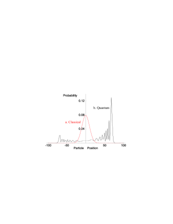
Figure 1: Probability distribution for a classical random walk (a) on a line after $N=100$ steps, as well as for a quantum walk (b) with initial state $|0\rangle\otimes|\!\!\uparrow\rangle$ and a Hadamard coin.

Let us consider the previous quantum walk, but now with two non-interacting particles on a line (not necessarily the same). If the particles are distinguishable and in a separable state, the position measurement of one particle will not change the probability distribution of the other, they are completely uncorrelated. On the other hand, if the particles are entangled, a new resource with no classical equivalent will be at our disposal.

The joint Hilbert space of our composite system is given by:

$$\mathcal{H}_{12}\equiv\mathcal{H}_{1}\otimes\mathcal{H}_{2}\equiv(\mathcal{H}_{P,1}\otimes\mathcal{H}_{C,1})\otimes(\mathcal{H}_{P,2}\otimes\mathcal{H}_{C,2}),$$ (5)

where $\mathcal{H}_{1}$ and $\mathcal{H}_{2}$ represent the Hilbert spaces of particles $1$ and $2$ respectively. Since the relevant degrees of freedom in our problem are the same for both particles, we have that both $\mathcal{H}_{1}$ and $\mathcal{H}_{2}$ are isomorphic to $\mathcal{H}$ defined earlier for the one-particle case. Note also that in the case of identical particles we have to restrict $\mathcal{H}_{12}$ to its symmetrical and antisymmetrical subspaces, respectively for bosons and fermions.

Let us then consider the case where both particles start the quantum walk in the same position, $0$, but with different coin states $|\!\!\downarrow\rangle$ and $|\!\!\uparrow\rangle$. In the case where the particles are in a pure separable state, our system’s initial state will be given by:

$$|\psi_{0}^{S}\rangle_{12}=|0,\downarrow\rangle_{1}|0,\uparrow\rangle_{2}.$$ (6)

We can also consider an initial pure state entangled in the coin degrees of freedom. In particular, we will consider the following two maximally entangled states:

$$|\psi_{0}^{\pm}\rangle_{12}=\frac{1}{\sqrt{2}}(|0,\downarrow\rangle_{1}|0,\uparrow\rangle_{2}\pm|0,\uparrow\rangle_{1}|0,\downarrow\rangle_{2}),$$ (7)

differing only by a relative phase. Note that if we were considering identical particles on the same point, our system would have to be described by these states, for bosons and fermions respectively.

Each step of this two-particles quantum walk will be given by:

$$\hat{U}_{12}=\hat{U}\otimes\hat{U},$$ (8)

where $\hat{U}$ is given by equation (1) and is the same for both particles. After $N$ steps, the state of the system will be, in the case of the initial conditions (6):

$$|\psi_{N}^{S}\rangle_{12}=\hat{U}^{N}_{12}\,|\psi_{0}^{S}\rangle_{12}=\hat{U}^{N}|0,\downarrow\rangle_{1}\hat{U}^{N}|0,\uparrow\rangle_{2}.$$ (9)

Fig. 2.a shows the joint probability distribution $P_{12}^{S}(i,j;N)$ for finding particle $1$ in position $i$ and particle $2$ in position $j$ for $N=30$ steps. Note that, since the particles are uncorrelated, $P_{12}^{S}(i,j;N)$ is simply the product of the two independent one-particle distributions:

$$P_{12}^{S}(i,j;N)=P^{S}_{1}(i;N)\times P^{S}_{2}(j;N),$$ (10)

where $P^{S}_{1}(i;N)$ is the probability distribution for finding particle $1$ in position $i$ after $N$ steps, and similarly for $P^{S}_{2}(j;N)$ and particle $2$. This can also be observed in Fig. 2.a, which is clearly the product of two distributions like the one in Fig. 1.b, one biased to the left for particle $1$ and the other to the right for particle $2$, accordingly with the initial conditions given by equation (6).

In the case of entangled particles, the state of the system after $N$ steps will be:

$$|\psi_{N}^{\pm}\rangle_{12}=\hat{U}^{N}_{12}\,|\psi_{0}^{\pm}\rangle_{12}$$

$$= \frac{1}{\sqrt{2}}\left(\hat{U}^{N}|0,\downarrow\rangle_{1}\,\hat{U}^{N}|0,\uparrow\rangle_{2}\pm\hat{U}^{N}|0,\uparrow\rangle_{1}\,\hat{U}^{N}|0,\downarrow\rangle_{2}\right).$$

The probability distribution for finding particle $1$ in position $i$ and particle $2$ in position $j$ in the “+” case, $P_{12}^{+}(i,j;N)$, is represented in Fig. 2.b, for $N=30$. Similarly, Fig. 2.c shows the distribution $P_{12}^{-}(i,j;N)$ of the “-” case, again for $N=30$. The effects of the entanglement are striking when comparing the three distributions in Fig. 2. In particular, we see that these effects significantly increase the probability of the particles reaching certain configurations on the line, which otherwise would be very unlikely to be occupied. In all cases, the maxima of the distributions occur around positions $\pm\,20$. In the “+” case it is most likely to find both particles together, whereas for “-” the former situation is impossible, and the particles will tend to finish as distant as possible from one another.

Let us now consider the individual particles in the entangled system. The state of each of them can be described by the reduced density operator $\hat{\rho}_{1,2}(N)\equiv Tr_{2,1}\left(|\psi_{N}^{\pm}\rangle_{12}\,\,{}_{12}\langle\psi_{N}^{\pm}|\right)$, which consists of an equal mixture of the one-particle states $\hat{U}^{N}|0,\downarrow\rangle$ and $\hat{U}^{N}|0,\uparrow\rangle$. Thus, given one particle, the probability to find it in position $i$ after $N$ steps is given by the following marginal probability distribution:

$$P_{1,2}^{\pm}(i;N)=\frac{1}{2}\left[P_{\downarrow}(i;N)+P_{\uparrow}(i;N)\right].$$ (12)

where $P_{\downarrow}(i;N)$ is the probability distribution for finding the particle in state $\hat{U}^{N}|0,\downarrow\rangle$ in position $i$ after $N$ steps, and similarly for $P_{\uparrow}(i;N)$ and a particle in state $\hat{U}^{N}|0,\uparrow\rangle$. Note that in the case of initial conditions (6) we have the marginal probabilities $P^{S}_{1}(i;N)=P_{\downarrow}(i;N)$ and $P^{S}_{2}(i;N)=P_{\uparrow}(i;N)$. But now, contrary to the separable case, the joint probability $P_{12}^{\pm}(i,j;N)$ is no longer the simple product of the two one-particle probabilities, as it contains information about the non-trivial correlations between the outcomes of the position measurement performed on each particle. Therefore, to investigate more quantitatively the difference between quantum walks with two distinguishable particles in a pure separable state and two entangled particles in their coin degree of freedom, we must look at joint (two-particle) rather than individual properties.

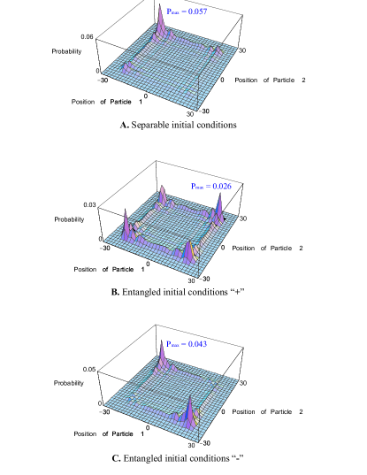
Figure 2: Two-particles probability distributions after $N=30$ steps for different initial conditions: (A) separable state $|\psi_{0}^{S}\rangle_{12}$; (B) $|\psi_{0}^{+}\rangle_{12}$ state; and (C) $|\psi_{0}^{-}\rangle_{12}$ state. Note the different vertical ranges.

First, let us consider the distance between the two particles, $\Delta^{S,\pm}_{12}$. For that, we define the random variables $x_{1}$ and $x_{2}$ as the outcomes of the (single particle) measurement of the position of particle $1$ and particle $2$ respectively, after $N$ steps of the quantum walk (they can take integer values between $N$ and $-N$). We can now define the distance as, for the three different initial conditions:

$$\Delta^{S,\pm}_{12}\equiv|x_{1}-x_{2}|.$$ (13)

The expectation value $\langle\Delta^{S,\pm}_{12}\rangle$ of the distance is given in Table 1 for different $N$. We see that in the “-” case the particles tend, on average, to end the quantum walk more distant to each other, whereas in the “+” case they tend to stay closer, and somewhere in between in the separable case. In fact, for fixed $N$, we always have:

$$\langle\Delta^{-}_{12}\rangle-\langle\Delta^{S}_{12}\rangle=\langle\Delta^{S}_{12}\rangle-\langle\Delta^{+}_{12}\rangle.$$ (14)

Let us now consider the correlation function between the spatial distribution of each of the two particles:

$$C^{S,\pm}(x_{1},x_{2})\equiv\langle x_{1}x_{2}\rangle-\langle x_{1}\rangle\langle x_{2}\rangle.$$ (15)

Clearly, in the case of the separable state (6) this correlation is always zero. For maximally entangled particles, the values of $C^{\pm}(x_{1},x_{2})$ are presented in Table 2 for different $N$. Given the symmetry of the $P_{12}^{\pm}$ distributions, we have that in those cases $\langle x_{1}\rangle=\langle x_{2}\rangle=0$. Thus, the sign difference in the correlation function expresses the tendency for the two particles in the “-” case to end the quantum walk on different sides of the line (with respect to its origin 0), and on the same side for the “+” case.

Finally, let us now calculate, for the different initial conditions, the probability of finding at least one particle in position $i$ after $N$ steps: $\mathcal{P}^{S,\pm}(i;N)$. This is clearly a joint property as it depends on both one-particle outcomes:

$$\mathcal{P}^{S,\pm}(i;N)=$$ (16)

$$= \sum_{j=-N}^{N}\left[P_{12}^{S,\pm}(i,j;N)+P_{12}^{S,\pm}(j,i;N)\right]-P_{12}^{S,\pm}(i,i;N)$$

$$= \left[P_{1}^{S,\pm}(i;N)+P_{2}^{S,\pm}(i;N)\right]-P_{12}^{S,\pm}(i,i;N)$$

$$= \left[P_{\downarrow}(i;N)+P_{\uparrow}(i;N)\right]-P_{12}^{S,\pm}(i,i;N).$$

Given a one-particle probability distribution, say $P_{\downarrow}(i;N)$ [note that $P_{\uparrow}(i;N)=P_{\downarrow}(-i;N)$], our probability $\mathcal{P}^{S,\pm}(i;N)$ decreases with the joint probability $P_{12}^{S,\pm}(i,i;N)$ and is maximal in the “-” case, as we always have $P_{12}^{-}(i,i;N)=0$. In fact, around the points $(20,20)$ and $(-20,-20)$ in Fig. 2 we clearly have:

$$\mathcal{P}^{-}(i;N)>\mathcal{P}^{S}(i;N)>\mathcal{P}^{+}(i;N).$$ (17)

We see that, by introducing entanglement in the initial conditions of our two-particles quantum walk, the probability of finding at least one particle in a particular position on the line can actually be better or worst than in the case where the two particles are independent. Note that in this case this does not depend on the particular amount of entanglement introduced, as both states in Eq. (7) are maximally entangled, but rather on their symmetry/relative phase.

Expectation value $\langle\Delta^{S,\pm}_{12}\rangle$ after $N$ steps
	Nb. of steps $N$			10		20		30		40		60		100
	Init. cond. $|\psi_{0}^{-}\rangle_{12}$			8.8		17.5		26.0		34.9		52.2		87.0
	Init. cond. $|\psi_{0}^{S}\rangle_{12}$			7.1		14.7		21.9		29.5		44.3		73.9
	Init. cond. $|\psi_{0}^{+}\rangle_{12}$			5.5		11.9		17.8		24.1		36.3		60.8

Table 1: Average distance $\langle\Delta^{S,\pm}_{12}\rangle$ after $N$ steps.

Correlation function $C^{S,\pm}(x_{1},x_{2})$ after $N$ steps
	Nb. of steps $N$	10		20		30		40		60		100
	Init. c. $|\psi_{0}^{-}\rangle_{12}$	-16.8		-69.8		-153.5		-276.2		-619.7		-1718.3
	Init. c. $|\psi_{0}^{S}\rangle_{12}$	0		0		0		0		0		0
	Init. c. $|\psi_{0}^{+}\rangle_{12}$	4.8		7.3		13.7		15.1		23.1		39.1

Table 2: Correlation function $C^{S,\pm}(x_{1},x_{2})$ after $N$ steps.

This work opens way for generalization in a number of ways. First, one could consider periodic or other boundary conditions on the line, or more general graphs Dorit . Note that the positions on the line of our two particles could also be interpreted as the position of a single particle doing the quantum walk on a regular two-dimensional lattice. More general coins could also be considered Hillery ; Oli , including entangling and non-balanced coins, as well as different initial states. One could also augment the number of particles, study these quantum walks in continuous time or in their asymptotic limit. Furthermore, also very interesting and promising is to investigate the use of multiparticle quantum walks in the design of quantum algorithms Mateus , or in solving mathematical or practical problems that could be encoded has a quantum walk, such as the estimation of the volume of a convex body Convex or the connectivity in a P2P network P2P .

Finally, some brief comments about implementations of our two-particles quantum walk on a line. The methods recently proposed for the single-particle case using cavity QED Knight , optical lattices Kendon or ion traps Travaglione could be adapted to our two-particles case. For instance, in the latter we could encode the coin states in the electronic levels of two ions and the position in their com or stretch motional modes: the coin flipping could then be obtained with a $\pi/2$ Raman pulse and the shift with a conditional optical dipole force Schaetz . Another possibility is to send two photons through a tree of balanced beam splitters which implement both the coin flipping and the conditional shift, again generalizing a scheme proposed for a single particle Hillery ; Kim . Note that this could be implemented with other particles as well, e.g. electrons, using a device equivalent to a beam splitter Yamamoto . Also very interesting, regardless of any particular method or technology, is the possibility of using two indistinguishable particles on the same line to implement our quantum walk. Say we encode the coin degrees of freedom in the polarization of two photons, or in the spin of two electrons: if the two particles start in the same position $0$, then they will be forced to be in state given by Eq. (7) (“+” for bosons and “-” for fermions). Although the particles will initially be only entangled in the mathematical sense (as they cannot be addressed to extract quantum correlations), this is a perfectly valid way of preparing the $|\psi_{0}^{+}\rangle_{12}$ and $|\psi_{0}^{-}\rangle_{12}$ initial states for our quantum walk, saving us the trouble of generating entangled pairs. Thus, the indistinguishability of identical particles appears once again as a resource for quantum information processing Omar , here in particular offering a way to simplify the preparation of the initial states for a two-particle quantum walk on a line.

In this article we introduced the concept of a quantum walk with two particles and studied it for the case of a discrete time walk on a line. Having more than one particle, we could now add a new feature to the walk: entanglement between the particles. In particular, we considered initial states maximally entangled in the coin degrees of freedom and with opposite symmetries, and compared them to the case where the two particles were initially unentangled and thus independent. We found that the entanglement in the coin states introduced spatial correlations between the particles, and that their average distance is larger in the “-” case than in the separable case, and is smaller in the “+” case. This could benefit algorithmic applications which require two marked sites to be reached which are known a priori to be on the opposite or on the same sides of a line. We also found that the introduction of entanglement could increase or decrease the probability to find at least one particle on a given point of the line. This increase could allow us to reach a marked site faster than with two unentangled quantum walkers. The entanglement in the initial conditions thus appears as a resource that we can tune according to our needs to enhance a given application (algorithmic or other) based on a quantum walk.

- (1) Y. Aharonov, L. Davidovich, and N. Zagury, Phys. Rev. A 48, 1687 (1993).
- (2) J. Kempe, Contemp. Phys. 44, 307 (2003).
- (3) N. Shenvi, J. Kempe, and K. B. Whaley, Phys. Rev. A 67, 052307 (2003); A. Ambainis, quant-ph/0311001 (2003).
- (4) A. M. Childs et al., Proc. 35th ACM Symposium on Theory of Computing (STOC), 59 (2003).
- (5) D. Aharonov, A. Ambainis, J. Kempe, and U. Vazirani, Proceedings 33rd ACM Symposium on Theory of Computation (STOC), 50 (2001); T.D. Mackay, S.D. Bartlett, L.T. Stephenson, and B.C. Sanders, J. Phys. A: Math. Gen. 35, 2745 (2002); B. Tregenna, W. Flanagan, R. Maile, and V. Kendon, New J. Phys. 5, 83 (2003).
- (6) M. Hillery, J. Bergou, and E. Feldman, Phys. Rev. A 68, 032314 (2003).
- (7) O. Buerschaper and K. Burnett, quant-ph/0406039 (2004).
- (8) P. Mateus and Y. Omar, work in progress.
- (9) M. Dyer, A. Frieze, and R. Kannan, Journal of the ACM 38, 1 (1991).
- (10) Q. Lv et al., Proceedings of the 16th ACM International Conference on Supercomputing (ICS), 84 (2002).
- (11) B. C. Sanders, S. D. Bartlett, B. Tregenna, and P. L. Knight, Phys. Rev. A 67, 042305 (2003).
- (12) W. Dür, R. Raussendorf, V. M. Kendon, and H.-J. Briegel, Phys. Rev. A 66, 052319 (2002).
- (13) B. C. Travaglione and G. J. Milburn, Phys. Rev. A 65, 032310 (2002).
- (14) T. Schaetz, work in progress.
- (15) H. Jeong, M. Paternostro, and M. S. Kim, Phys. Rev. A 69, 012310 (2004).
- (16) R. C. Liu, B. Odom, Y. Yamamoto, and S. Tarucha, Nature 391, 263 (1998).
- (17) Y. Omar, N. Paunković, S. Bose, and V. Vedral, Phys. Rev. A 65, 062305 (2002); N. Paunković, Y. Omar, S. Bose and V. Vedral, Phys. Rev. Lett. 88, 187903 (2002).