Submicrometer position control of single trapped neutral atoms

Abstract

We optically detect the positions of single neutral cesium atoms stored in a standing wave dipole trap with a sub-wavelength resolution of 143 nm rms. The distance between two simultaneously trapped atoms is measured with an even higher precision of 36 nm rms. We resolve the discreteness of the interatomic distances due to the 532 nm spatial period of the standing wave potential and infer the exact number of trapping potential wells separating the atoms. Finally, combining an initial position detection with a controlled transport, we place single atoms at a predetermined position along the trap axis to within 300 nm rms.

Precision position measurement and localization of atoms is of great interest for numerous applications and has been achieved in and on solids using e.g. scanning tunnelling microscopy Binnig99 , atomic force microscopy Giessibl03 , or electron energy-loss spectroscopy imaging Suenaga00 . However, if the application requires long coherence times, as is the case in quantum information processing DiVincenzo95 and Ekert96 or for frequency standards, the atoms should be well isolated from their environment. This situation is realized for ions in ion traps, freely moving neutral atoms, or neutral atoms trapped in optical dipole traps. For the case of ions, positions Walther01 ; Blatt02 and distances Wineland03 have been optically measured and controlled with a sub-optical wavelength precision. Similar precision has been reached in an all-optical position measurement of freely moving atoms Thomas95 . Dipole traps, operated as optical tweezers, have been used to precisely control the position of individual neutral atoms Kuhr01 ; Bergamini04 . To our knowledge, however, a sub-micrometer position or distance measurement has so far not been achieved in this case. Such a control of the relative and absolute position of single trapped neutral atoms, however, is an important prerequisite for cavity quantum electrodynamics as well as cold collision experiments, aiming at the realization of quantum logic operations with neutral atoms.

Here, we report on the measurement and control of the position of single neutral atoms stored in a standing wave optical dipole trap (DT). The positions of the atoms are inferred from their fluorescence using high resolution imaging optics in combination with an intensified CCD camera (ICCD). The absolute position of individual atoms along the DT is measured with a precision of 143 nm rms. The relative position of the atoms, i.e. their separation, is determined more accurately by averaging over many measurements, yielding a relative position uncertainty of 36 nm. Due to this high resolution, we can resolve the discreteness of the distribution of interatomic distances in the standing wave potential even though our DT is formed by a Nd:YAG laser with potential wells separated by only 532 nm. This allows us to determine the exact number of potential wells between simultaneously trapped atoms. Finally, using our “optical conveyor belt” technique Kuhr01 ; Schrader01 we transport individual atoms to a predetermined position along the DT axis with an accuracy of 300 nm, thereby demonstrating a high degree of control of the absolute atom position.

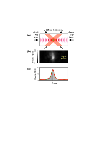
Figure 1: Determination of the position of a single trapped atom. (a) An atom stored in the standing wave dipole trap is illuminated with an optical molasses (schematic drawing). (b) ICCD image of one atom stored in the DT with an exposure time of 1 s. The observed fluorescence spot corresponds to about 200 detected photons. (c) To determine the position of the atom along the DT axis, the pixel counts are binned in the vertical direction. The solid line corresponds to the line spread function of our imaging optics and reveals the absolute position $x_{\mathrm{atom}}$ of the atom. For comparison, the dashed line shows a fit with a simple Gaussian (see text for details).

We will only give the essential details of our experimental set-up. A more exhaustive description can e.g. be found in Schrader01 ; Miroshnychenko03 . Our standing wave dipole trap is formed by the interference pattern of two counter-propagating Nd:YAG laser beams ($\lambda=1.064\,\mu$m) with a waist of $2w_{0}=38\,\mu$m and a total optical power of $2$ W. They produce a trapping potential with a maximal depth of $U_{\mathrm{max}}/k_{\mathrm{B}}=0.8$ mK for cesium atoms. Mutually detuning the frequency of the two laser beams moves the trapping potential along the DT axis and thereby transports the atoms Kuhr01 ; Schrader01 ; Miroshnychenko03 . The laser frequency is changed by acousto-optic modulators (AOMs), placed in each beam and driven by a digital dual-frequency synthesizer. The DT is loaded with cold atoms from a high-gradient magneto-optical trap (MOT). We deduce the exact number of atoms in the MOT from their discrete fluorescence levels detected by an avalanche photodiode. The transfer efficiency between the traps is better than 99 %.

In order to obtain fluorescence images of the atoms in the DT, we illuminate them with a near-resonant three-dimensional optical molasses, see Fig. 1(a). The molasses counteracts heating through photon scattering, resulting in an atom temperature of about 70 $\mu$K. The storage time in the trap is about $25$ s, limited by background gas collisions. The fluorescence light is collected by a diffraction limited microscope objective Alt02 and imaged onto the ICCD Miroshnychenko03 . One detected photon (quantum efficiency approx. 10 % @ 852 nm) generates on average 350 counts on the CCD chip, and one $13\ \mu\mathrm{m}\times 13\ \mu\mathrm{m}$ CCD pixel corresponds to $0.933\,(\pm 0.004)\,\mu$m in the object plane.

Figure 1(b) shows an ICCD image of a single atom stored in the DT with an exposure time of 1 s. This exposure time is much longer than the timescale of the thermal position fluctuations of the atom inside the trap. Therefore, the vertical width of the fluorescence spot, i.e. perpendicular to the DT axis, is essentially defined by the spread of the Gaussian thermal wave packet of the atom in the radial direction of the trap. In the axial direction of the DT, the wave packet has a much smaller $1/\sqrt{e}$-halfwidth of only $\Delta x_{\mathrm{therm}}=35$–50 nm, depending on the depth of the DT. In addition to these thermal fluctuations, the axial position of the standing wave itself is fluctuating by $\sigma_{\mathrm{fluct}}(1\,\mathrm{s})=42\,(\pm 13)$ nm during the 1 s exposure time due to drifts and acoustic vibrations of the optical setup (see below). The horizontal $1/\sqrt{e}$-halfwidth of the detected fluorescence peak, $w_{\mathrm{ax}}=1.3(\pm$0.15) $\mu$m, is much larger and is caused by diffraction within the imaging optics and a slight blurring in the intensification process of the ICCD. Compared to the point spread function of our imaging system, $\Delta x_{\mathrm{therm}}$ and $\sigma_{\mathrm{fluct}}$ have thus a negligible effect on $w_{\mathrm{ax}}$. Note, however, that all the atom positions and the distances between atoms given in the following refer to the center of the Gaussian thermal wave packets of the atoms.

The ICCD image is characterized by its intensity distribution $I(\tilde{x}_{i},\tilde{y}_{j})$, where $\tilde{x}_{i}$ and $\tilde{y}_{j}$ denote the horizontal and vertical position of pixel $\{i,j\}$, respectively. In order to determine the horizontal position $\tilde{x}_{\mathrm{atom}}$ of the fluorescence peak from the ICCD image, we bin $I(\tilde{x}_{i},\tilde{y}_{j})$ in the vertical direction. Neglecting noise for the moment, this yields $I(\tilde{x}_{i})=\sum_{j}I(\tilde{x}_{i},\tilde{y}_{j})\propto L(\tilde{x}_{i}-\tilde{x}_{\mathrm{atom}})$, where $L(\tilde{x})$ is the line spread function (LSF) of our imaging optics. Without distortions, the object coordinate $x_{\mathrm{atom}}$ and the image coordinate $\tilde{x}_{\mathrm{atom}}$ are connected by the relation $x_{\mathrm{atom}}=(\tilde{x}_{\mathrm{atom}}-\widetilde{\mathcal{O}}_{x})/M$, where $\widetilde{\mathcal{O}}_{x}$ is the image coordinate of the origin and $M$ is the magnification of our imaging optics. In general, $\widetilde{\mathcal{O}}_{x}$ and $M$ have to be calibrated from independent measurements. In the present case, however, no physical point in space is singled out as an origin and we arbitrarily set $\widetilde{\mathcal{O}}_{x}\equiv 0$.

Our LSF is position-independent and is well described by a sum of two Gaussians with a ratio of 4.4:1 in heights and 1:3.2 in widths, with a slight horizontal offset with respect to each other, see Fig. 1(c). We define $\tilde{x}_{\mathrm{atom}}$ as the position of the maximum of this LSF. In our experiment, it is determined by fitting a simple Gaussian to the fluorescence peak. This procedure has been chosen because it can be carried out in a fast automated way, yielding information about the atom position during the running experimental sequence. Assuming pure shot noise, this allows to determine $x_{\mathrm{atom}}$ with a statistical error of

$$\Delta x_{\mathrm{stat}}=1.44\,w_{\mathrm{ax}}/\sqrt{N_{\mathrm{ph}}},$$ (1)

where $N_{\mathrm{ph}}$ is the number of detected photons and the numerical factor has been determined by a numerical simulation taking into account the experimental LSF and the bin size. In the experiment the value of $N_{\mathrm{ph}}$ depends on the illumination parameters. Here, $N_{\mathrm{ph}}=200(\pm 30)$ photons per second per atom, so that $\Delta x_{\mathrm{stat}}=130\,(\pm 20)$ nm. Our simulation also yields a constant position offset of 42 nm of the fitted center of the Gaussian with respect to the maximum of the LSF, due to the slight asymmetry of our LSF. This offset only leads to a global shift of $\widetilde{\mathcal{O}}_{x}$ and is irrelevant for our analysis.

In addition to the statistical error, two further sources influence the precision of the position detection: the background noise of our ICCD image and the position fluctuations of the DT. The background in Fig. 1 originates in equal proportions from stray light and the read-out process of the ICCD, yielding a total offset of $2300(\pm 300)$ counts per bin for 1 s exposure time. The noise of $300$ counts per bin introduces an additional uncertainty of $\Delta x_{\mathrm{backgr}}=15$ nm to the fitted peak center.

The atom position is subject to position fluctuations of the DT, $\sigma_{\mathrm{fluct}}$. Since $\sigma_{\mathrm{fluct}}$ cannot be extracted from the ICCD image, we determine it in an independent measurement. For this purpose, we mutually detune the two trap beams and overlap them on a fast photodiode. From the phase of the resulting beat note we infer the phase variations $\phi(t)$ of the standing wave with a 300 kHz bandwidth. The standard deviation of $\phi(t)$, $\sigma_{\phi}(\tau)$, is directly related to the position fluctuations of the DT during the time interval $\tau$ by $\sigma_{\mathrm{fluct}}(\tau)=\lambda/2\cdot\sigma_{\phi}(\tau)/2\pi$. We have found $\sigma_{\mathrm{fluct}}(1\,\mathrm{s})=42\,(\pm 13)$ nm. Thus, using the approximation of Gaussian-distributed position fluctuations, which we have checked to be valid to better than 1 % in our case, the position uncertainty immediately after the 1 s exposure time is given by

$$\Delta x_{\mathrm{atom}}^{2}(1\,\mathrm{s})=\Delta x_{\mathrm{stat}}^{2}+\Delta x_{\mathrm{backgr}}^{2}+\sigma_{\mathrm{fluct}}^{2}(1\,\mathrm{s})\ ,$$ (2)

yielding $\Delta x_{\mathrm{atom}}(1\,\mathrm{s})=140\,(\pm 20)$ nm.

Finally, the read-out and the data analysis of the image take an additional 0.5 s during which $x_{\mathrm{atom}}$ is further subject to position fluctuations of the DT. This increases the variance of the position measurement by $2\sigma_{\mathrm{fluct}}^{2}(0.5\,\mathrm{s})$. Thus, we can determine the absolute position of the trapped atom with a precision of $\Delta x_{\mathrm{atom}}(1.5\,\mathrm{s})=143\,(\pm 20)$ nm within 1.5 s (1 s exposure time plus 0.5 s read-out and data analysis). Our analysis shows that this precision cannot be significantly increased by extending the exposure time because the benefit of the higher photon statistics for longer times is counteracted by the increase in $\sigma_{\mathrm{fluct}}(\tau)$.

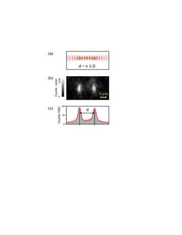
Figure 2: Determination of the distance between atoms. (a) Two atoms in the standing wave dipole trap have a separation of $n\lambda/2$ with $n$ integer. (b) After loading the atoms into the DT, we successively take many camera pictures of the same pair of atoms. (c) From each picture (exposure time 1 s) we determine the positions of the atoms and their separation $d$. Averaging over many measurements of $d$ reduces the statistical error and allows us to infer $n$.

While for some applications the absolute position of the atoms must be known to the highest possible precision, other experiments, like e.g. controlled cold collisions Mandel03 , require a precise knowledge of the separation $d$ between atoms. In the following we will show that in our case this separation can be more precisely determined than the absolute positions of the individual atoms. The reason is that DT fluctuations equally influence all simultaneously trapped atoms and therefore do not affect the separation between them. Thus, this distance can be averaged over many measurements. Given the precision of the peak detection, the uncertainty of the separation $d$ between two atoms determined from one picture should be $\Delta d^{2}=2(\Delta x_{\mathrm{stat}}^{2}+\Delta x_{\mathrm{backgr}}^{2})$. Averaging the results from $N_{\mathrm{pic}}$ images should then reduce the statistical error of the mean value $\bar{d}$ to $\Delta\bar{d}=\Delta d/\sqrt{N_{\mathrm{pic}}}$. Since the data processing in this case is carried out at a later stage, we use the experimentally established LSF [see Fig. 1(c)] for fitting the fluorescence peaks. For the case of partially overlapping fluorescence spots $(d\lesssim 10~{}\mu\mathrm{m})$, this method yields more precise results for the two atom positions than fitting a simple Gaussian. For $d\lesssim 4~{}\mu\mathrm{m}$ the increasing overlap reduces the precision of the position determination. We have therefore restricted our investigations to the case where the atoms are separated by more than 4 $\mu$m.

To realize this scheme experimentally, we first load the DT with two atoms, see Fig. 2(a). We then typically take $N_{\mathrm{pic}}=10$ successive camera pictures of the same pair before one of the two atoms leaves the trap. In these experiments, we detect $N_{\mathrm{ph}}=270(\pm 30)$ photons per second per atom. From each picture we determine the distance $d$ between the atoms, see Fig. 2 (b) and (c), and then calculate its mean value $\bar{d}$ and its standard deviation $\Delta d$ for each pair. Our measured value of $\Delta d=135\,(\pm 30)$ nm is in resonable agreement with the expected value of $\sqrt{2}\Delta x_{\mathrm{stat}}=160(\pm 25)$ nm, inferred from Eq. (1), thereby confirming its validity.

By averaging the distance over about $N_{\mathrm{pic}}=10$ images per atom pair, the uncertainty in $\bar{d}$ should therefore be reduced to $\Delta\bar{d}\approx 40$ nm. Now, the separation of trapped atoms equals $d=n\lambda/2$ with $n$ integer, see Fig. 2(a). If $d$ can be measured with a precision $\Delta d\ll\lambda/2$, its distribution should therefore reveal the standing wave structure of the DT. Indeed, the $\lambda/2$ period is strikingly apparent in Fig. 3 which shows the cumulative distribution of mean distances $\bar{d}$ between atoms.

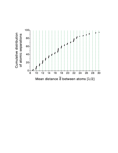
Figure 3: Cumulative distribution of separations between atoms in the dipole trap measured with the scheme presented in Fig. 2. In order to resolve the periodic structure of the trap, we reduce the statistical error in the measurement of the atomic separation by averaging over more than 10 distance measurements for each atom pair. The discretization of the distances to $n\lambda/2$ is clearly visible in the data. Our resolution is thus sufficient to determine the exact number of potential wells between any two optically resolved atoms.

The resolution of our distance measurements can be directly inferred from the finite width of the steps observed in Fig. 3, yielding $\Delta\bar{d}=36\,(\pm 12)$ nm. This result proves that we can determine the exact number of potential wells between two optically resolved atoms, a situation that so far seemingly required much longer (e.g. CO₂) trapping laser wave lengths Scheunemann00 .

Using our scheme to precisely measure the position of an atom, we now demonstrate active control of its absolute position along the DT axis. This is realized by transporting the atom to a predetermined position $x_{\mathrm{target}}$ by means of our optical conveyor belt. Initially, we determine the position of the atom and its distance $L$ from $x_{\mathrm{target}}$ from an ICCD image by fitting a simple Gaussian. To move the atom to $x_{\mathrm{target}}$, it is uniformly accelerated along the first half of $L$ and uniformly decelerated along the second half with an acceleration of $a=\pm 1000$ m/s² Schrader01 . To confirm the successful transport to $x_{\mathrm{target}}$, we take a second image of the atom and measure its final position. We repeat the same experiment about 400 times with a single atom each time.

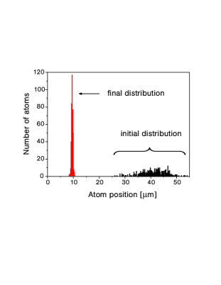
Figure 4: Absolute position control of single trapped atoms. The histogram shows the accumulative data of about 400 experiments carried out with one single atom at a time. Transfer of the atoms from the MOT to the DT yields the broad distribution on the right (standard deviation $5.0\ \mu$m). We transport the atoms to the target position at $x_{\mathrm{target}}=9.5\ \mu$m with a precision of 300 nm rms (narrow distribution on the left).

Because the atoms are randomly loaded from the MOT into the DT, the distribution of their initial positions, see Fig. 4, has a standard deviation of $5.0\,(\pm 0.3)\,\mu$m, corresponding to the MOT radius. After the transport, the width of the distribution of the final positions is drastically reduced to $\sigma_{\mathrm{control}}=300\,(\pm 15)$ nm. This width is limited by the errors in determining the final and initial position of the atom, by the transportation error $\sigma_{\mathrm{transp}}$, resulting from the discretization error of our digital dual-frequency synthesizer which drives the optical conveyor belt, and by the DT position drifts, $\sigma_{\mathrm{drift}}$, during the typical time of 1.5 s between the two successive exposure intervals. From the above DT phase measurement we find $\sigma_{\mathrm{drift}}=140\,(\pm 20)$ nm. Assuming that

$$\sigma_{\mathrm{control}}=\sqrt{2\Delta x_{\mathrm{stat}}^{2}+\sigma_{\mathrm{drift}}^{2}+\sigma_{\mathrm{transp}}^{2}},$$ (3)

we calculate that $\sigma_{\mathrm{transp}}=190\,(\pm 25)$ nm, comparable to the statistical error.

In addition to statistical errors, the accuracy of the position control is subject to systematic errors. The predominant systematic error stems from the calibration of our length scale. In the present case, a relative calibration error of $0.4$ % results in a $120$ nm shift of the final positions with respect to the target position after a transport over $L\approx 30\,\mu$m. However, this error could be reduced by improving the accuracy of the calibration.

Summarizing, we have realized a detection scheme for the absolute and relative position of individual atoms stored in our standing wave dipole trap, yielding sub-micrometer resolution. We have shown that this scheme allows us to measure the exact number of potential wells separating simultaneously trapped atoms in our 532 nm-period standing wave potential. We have furthermore used our position detection scheme to transport an atom to a predetermined position with a sub-optical wavelength accuracy. These results represent an important step towards experiments in which the relative or absolute position of single atoms has to be controlled to a high degree. For example, we aim to use this technique for a deterministic coupling of atoms to the mode of a high-Q optical resonator in order to realize quantum logic operations Walther01 ; Blatt02 ; Schrader04 ; You03 . Furthermore, knowing the exact number of potential wells separating the atoms, we can now attempt to control this parameter by placing atoms into specific potential wells of our standing wave using additional optical tweezers. Finally, the demonstrated high degree of control allows us to envision the implementation of controlled cold collisions between optically resolved individual atoms by means of spin-dependent transport Mandel03 .

We acknowledge valuable discussions with V. I. Balykin. This work was supported by the Deutsche Forschungsgemeinschaft and the EC (IST/FET/QIPC project “QGATES”). I. D. acknowledges funding from INTAS. D. S. acknowledges funding by the Deutsche Telekom Stiftung.

References

- (1) G. Binnig and H. Rohrer, Rev. Mod. Phys. 71, S324 (1999)
- (2) F. J. Giessibl, Rev. Mod. Phys. 75, 949 (2003)
- (3) K. Suenaga et al., Science 290, 2280 (2000)
- (4) D. P. DiVincenzo, Science 270, 255 (1995); A. Ekert and R. Jozsa, Rev. Mod. Phys. 68, 733 (1996)
- (5) G. R. Guthöhrlein et al., Nature 414, 49 (2001)
- (6) A. B. Mundt et al., Phys. Rev. Lett. 89, 103001 (2002)
- (7) D. Leibfried et al., Nature 422, 412 (2003)
- (8) J. E. Thomas and L. J. Wang, Phys. Rep. 262, 311 (1995)
- (9) S. Kuhr et al., Science 293, 278 (2001)
- (10) S. Bergamini et al., J. Opt. Soc. Am. B 21, 1889 (2004)
- (11) D. Schrader et al., Appl. Phys. B 73, 819 (2001)
- (12) Y. Miroshnychenko et al., Optics Express 11, 3498 (2003)
- (13) W. Alt, Optik 113, 142 (2002)
- (14) O. Mandel et al., Nature 425, 937 (2003)
- (15) R. Scheunemann et al., Phys. Rev. A 62, 051801(R) (2000)
- (16) D. Schrader et al., Phys. Rev. Lett. 93, 150501 (2004)
- (17) L. You, X. X. Yi, and X. H. Su, Phys. Rev. A 67, 032308 (2003)