Ground state entanglement of the BCS model

Abstract

The concept of local concurrence is used to quantify the entanglement between a single qubit and the remainder of a multi-qubit system. For the ground state of the BCS model in the thermodynamic limit the set of local concurrences completely describe the entanglement. As a measure for the entanglement of the full system we investigate the Average Local Concurrence (ALC). We find that the ALC satisfies a simple relation with the order parameter. We then show that for finite systems with fixed particle number, a relation between the ALC and the condensation energy exposes a threshold coupling. Below the threshold, entanglement measures besides the ALC are significant.

Quantification of entanglement remains as a major challenge in quantum information theory. For a state of a bi-partite system, it is well known that a measure for the entanglement between the two subsystems is given by the von Neumann entropy pr . For a two-qubit system, the concurrence hw has been introduced as an alternative measure which is related to the von Neumann entropy in a bijective manner. In the language of spin-1/2 particles, concurrence can be described in terms of a time-reversal operation. Using this concept, generalisations of concurrence have been proposed for multi-qubit systems and in particular they have been applied to quantify the entanglement of the ground state of the BCS model in the thermodynamic limit g ; md , which breaks time-reversal symmetry due to broken gauge symmetry.

In this Letter we adopt a different approach to investigate the ground state entanglement of the BCS model. We will use the notion of local concurrence which is defined in analogy with the functional relation that exists between concurrence and von Neumann entropy for a two qubit system (cf. ckw ). It is a measure of the entanglement between a single qubit and the remainder of the system. We then define an entanglement measure which is the Average Local Concurrence (ALC). The ALC satisfies the properties of an entanglement monotone (EM): it vanishes for a state if and only if that state is a product state, is invariant under local unitary transformations, and does not increase on average under local operations assisted by classical communication.

For multi-qubit systems the number of independent EMs is the same as the number of non-local invariants ging , growing exponentially with system size ($2^{L+1}-3L-2$ where $L$ is the number of qubits lps ; kem ). It is therefore useful to identify EMs which can be related to physical aspects of the system. In the thermodynamic limit we will show that the ALC for the ground state of the BCS model displays a simple relationship with the magnitude of the order parameter. For finite systems the order parameter vanishes, so we may use the ALC in lieu of the order parameter. Our investigation of a relationship between the ground state ALC and the condensation energy exposes a threshold coupling which signifies the onset of entanglement not measured by the local concurrences.

To study the entanglement of any pure state we can examine the von Neumann entropy. Consider a general quantum system comprised of $L$ qubits and a partition into two subsystems denoted $A$ and $B$. For any pure state density matrix $\rho$ the entanglement $\mathcal{E}_{AB}(\rho)$ between $A$ and $B$ is given by the von Neumann entropy

$$\mathcal{E}_{AB}(\rho)=-{\rm tr}(\rho_{A}\log\rho_{A})=-{\rm tr}(\rho_{B}\log\rho_{B})$$

where the logarithm is taken base 2 and $\rho_{A}$ is the reduced density matrix obtained from $\rho$ by taking the partial trace over the state space of subsystem $B$. The reduced density matrix $\rho_{B}$ is defined analogously.

Now we make precise the definition of local concurrence in a general context. Hereafter we will only deal with the particular case when the subsystem $A$ denotes a single qubit (say the $j$th qubit) and $B$ denotes the remainder of the system. For this case we will write $\rho_{j}$ for $\rho_{A}$ and $\mathcal{E}_{j}(\rho)$ for $\mathcal{E}_{AB}(\rho)$. In such an instance we have $\mathcal{E}_{j}(\rho)=-\lambda_{j}^{+}\log(\lambda_{j}^{+})-\lambda_{j}^{-}\log\lambda_{j}^{-}$ where $\lambda_{j}^{\pm}$ denote the two eigenvalues of $\rho_{j}$. Using the fact that ${\rm tr}(\rho_{j})=1$ and that the eigenvalues of $\rho_{j}$ lie in the interval $[0,1]$ means that we can always parameterise them as $\lambda_{j}^{\pm}=\left(1\pm\sqrt{1-C^{2}_{j}}\right)/2$ with $C_{j}\in[0,\,1]$. For a two-qubit system $C=C_{1}=C_{2}$ is precisely the concurrence hw , so it is natural to call the $C_{j}$ for the $L$-qubit system the local concurrences (cf. ckw ). In terms of Pauli matrices it can be determined that $\rho_{j}=\left(I+\sum_{\alpha=x,y,z}\left<\sigma_{j}^{\alpha}\right>\sigma^{\alpha}_{j}\right)/2$ giving the local concurrence as

$$C_{j}=\sqrt{1-\sum_{\alpha=x,y,z}\left<\sigma_{j}^{\alpha}\right>^{2}}.$$ (1)

For the ground state of the BCS model we will establish a correspondence between each local concurrence and a certain correlation function $\tilde{C}_{j}$ (see (6) below) describing the fluctuation in the Cooper pair occupation numbers. An advantage of this approach is that it applies equally to the thermodynamic limit where gauge symmetry is broken, and for finite systems where there is no broken symmetry. We obtain analytic results for the ALC in two extreme cases; (i) the thermodynamic limit and (ii) the case of a single Cooper pair in a system with two single particle energy levels. Between these extremes we investigate the ALC in terms of the exact solution of the model provided by the Bethe ansatz r , which facilitates the calculation of correlation functions zlmg ; lzmg and in turn the ALC.

The reduced BCS model. The reduced BCS Hamiltonian has received much attention as a result of the effort to understand pairing correlations in nanoscale metallic systems ds ; vd . The Hamiltonian reads

$$H_{\rm{BCS}} = \sum_{j=1}^{L}\epsilon_{j}n_{j}-d\lambda\sum_{j\neq k}^{L}c_{j+}^{\dagger}c_{j-}^{\dagger}c_{k-}c_{k+}.$$ (2)

Above, $j=1,\dots,{L}$ labels a shell of doubly degenerate single particle energy levels with energies $\epsilon_{j}$, $d$ is the mean level spacing and $\lambda$ is the dimensionless coupling. The operators $c_{j\pm},\,c^{\dagger}_{j\pm}$ are the annihilation and creation operators for electrons at level $j$ where the labels $\pm$ refer to pairs of time-reversed states and $n_{j}=c^{\dagger}_{j+}c_{j+}+\ c^{\dagger}_{j-}c_{j-}$ is the electron number operator for level $j$. Throughout we will only consider systems at half-filling. The physical properties predicted by the model are quite different in the superconducting (SC) regime ($d\ll\tilde{\Delta}$, where $\tilde{\Delta}$ is the bulk gap, defined below) and the fluctuation dominated (FD) regime ($d\gg\tilde{\Delta}$), the latter being the case for nanoscale systems. For the SC regime the variational BCS ansatz using mean-field theory can be used to determine the ground state properties. However, the mean-field approximation is not justified in the FD regime, where quantum fluctuations are significant.

The condensation energy $E^{c}$ is defined as the energy loss relative to the energy of the uncorrelated state (i.e. the ground state energy at $\lambda=0$, or equivalently the energy expectation value of the Fermi sea). In the language of ddb , it is equivalent to the entanglement gap for this model. Intuitively, the entanglement gap gives an indication of the ground state entanglement of the system. By definition, it is zero if and only if the ground state is not entangled. It is thus desirable to determine how the entanglement gap (or equivalently the condensation energy) relates to EMs. It is known that the condensation energy is extensive in the SC regime, intensive in the FD regime, but with entirely smooth behaviour in the crossover ds ; vd . Below we will use a relation between condensation energy and the ALC to establish that a threshold coupling exists which marks qualitative differences in the ground state in terms of entanglement. An important quantity in our subsequent analysis will be played by the dimensionless condensation energy per electron, defined by $\tilde{E}=E^{c}/\omega_{D}L$.

Next we discuss the decomposition of the Hilbert space into subsystems. At each energy level $\epsilon_{j}$ there are four independent states; $\left|0\right>,\,c^{\dagger}_{+}\left|0\right>,\,c^{\dagger}_{-}\left|0\right>,\,c^{\dagger}_{+}c^{\dagger}_{-}\left|0\right>$. These states serve as a ququadrit, which can be further decomposed into two qubits through the identification $\left|0\right>\equiv\left|00\right>,\,c^{\dagger}_{+}\left|0\right>\equiv\left|10\right>,\,c^{\dagger}_{-}\left|0\right>\equiv\left|01\right>,\,c^{\dagger}_{+}c^{\dagger}_{-}\left|0\right>\equiv\left|11\right>$ z ; zw . In the ground state all electrons are paired, so there is zero probability of observing a single electron at any level $\epsilon_{j}$. Thus for the ground state each level $\epsilon_{j}$ gives rise to a two-state system with basis $\left|0\right>,\,c^{\dagger}_{+}c^{\dagger}_{-}\left|0\right>$, and each ququadrit serves as an effective qubit.

The grand canonical ensemble. The conventional BCS theory bcs employs a grand canonical ensemble, where the electron number is not fixed, using the well-known variational ground state ansatz

$$\left|\rm{BCS}\right>=\prod_{j=1}^{L}(u_{j}I+e^{i\theta}v_{j}c_{j+}^{\dagger}c_{j-}^{\dagger})\left|0\right>$$ (3)

with $u_{j},\,v_{j}$ real and satisfying $u_{j}^{2}+v_{j}^{2}=1$. Including only those levels within the cut-off given by the Debye frequency $\omega_{D}$ (i.e. $|\epsilon_{j}|\leq\omega_{D}$ where the Fermi level is $\epsilon_{F}=0$), minimisation of the expectation value of the energy for (3) gives

$$4u_{j}^{2}v_{j}^{2} = {\tilde{\Delta}^{2}}/{(\epsilon_{j}^{2}+\tilde{\Delta}^{2})}$$ (4)

where $\tilde{\Delta}=\omega_{D}/\sinh(1/\lambda)$ is the bulk gap. Unless stated otherwise we assume that the levels $\epsilon_{j}$ are uniformly distributed. It can then be deduced that $\tilde{E}=(\coth(1/\lambda)-1)/2$.

With respect to the decomposition of (3) into ququadrits discussed above, it is a product state and thus not entangled. There is however entanglement within each ququadrit subsystem. Expressing the state of a ququadrit as $u\left|00\right>+v\,e^{i\theta}\left|11\right>$ it is easily determined that the concurrence is $C=2|uv|$. Thus for the state (3) we may define $L$ local concurrences $C_{j}$ associated with each level $j$, which quantify the entire entanglement content of the state. Remarkably, most of the $2^{L{+}1}{-}3L{-}2$ independent EMs are zero. Note that the definition of local concurrence here is not the same as the definition of partial concurrence in md based on the notion of broken time-reversal symmetry of (3) (see also g ). A simple choice for an EM which reflects the overall ground state entanglement is the ALC, $\overline{C}={L^{-1}}\sum_{j=1}^{L}C_{j}$. We remark that $\overline{C}$ only quantifies bi-partite entanglement, and not multi-partite entanglement ckw ; lps ; kem . However (3) has no multi-partite entanglement. In the thermodynamic limit $d\rightarrow 0$ with $Ld=2\omega_{D}$ finite we can compute the ALC as

$$\overline{C} = \frac{\int_{-\omega_{D}}^{\omega_{D}}f(\epsilon)\mu(\epsilon)d\epsilon}{\int_{-\omega_{D}}^{\omega_{D}}\mu(\epsilon)d\epsilon}$$ (5)

with $f(\epsilon)=\tilde{\Delta}/(\sqrt{\epsilon^{2}+\tilde{\Delta}^{2}})$ and $\mu(\epsilon)\geq 0$ a density function for the distribution of the single particle energy levels. For the case $\mu(\epsilon)=1$ it is straightforward to determine that the ALC is $\overline{C}={1}/({\lambda\sinh(1/\lambda)})$. Recalling vd that the order parameter is given by $\Delta=\lambda d\sum_{j=1}^{L}\left<c_{j-}c_{j+}\right>$ we have $|\Delta|=\lambda\omega_{D}\overline{C}$. This last relation reflects the fact that superconducting order arises from the instability of the Fermi sea due to Cooper pairing, which also results in the emergence of entanglement in the ground state. Additionally we find $2{d\tilde{E}}/{d\lambda}=\overline{C}^{2}$. For the canonical case (i.e. a finite system with fixed electron number) the order parameter vanishes, but one can alternatively study the extent to which ‘superconducting order’ survives through the study of certain correlation functions vd , which we will show can be used to compute the ALC.

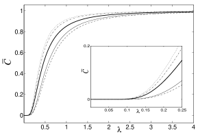
Figure 1: The ALC as a function of the dimensionless coupling $\lambda$ in the thermodynamic limit for various distributions $\mu(\epsilon)$ of the single particle levels. The results shown are for, in increasing order of local density about the Fermi level, $\mu(\epsilon)=\epsilon^{2}$ (dash), $\mu(\epsilon)=|\epsilon|$ (solid), $\mu(\epsilon)=1$ (bold), $\mu(\epsilon)=\omega^{2}_{D}-\epsilon^{2}$ (dash-dot) and $\mu(\epsilon)=\omega_{D}-|\epsilon|$ (dot). For each of these cases the expression (5) can be evaluated analytically.

We introduce the correlators describing the fluctuation in Cooper pair occupation:

$$\tilde{C}_{j} = \sqrt{\left<n_{j}^{2}\right>-\left<n_{j}\right>^{2}}=\sqrt{\left<2-n_{j}\right>\left<n_{j}\right>}.$$ (6)

These correlators can be directly evaluated for the variational wavefunction (3) giving $\tilde{C}_{j}=2\left|u_{j}v_{j}\right|=C_{j}$, so the local concurrence is precisely the fluctuation of the Cooper pair occupation. These fluctuations are localised within the range $\tilde{\Delta}$ of the Fermi level as given by (4). The behaviour of the ALC is strongly influenced by the density of levels about the Fermi level, as depicted in Fig. 1. Hereafter we will only consider the case of uniform distribution of the levels to simplify the analysis.

In the thermodynamic limit (3) becomes the exact ground state and the finite size corrections are of order $1/L$ a . For systems with large but finite electron number in the SC regime, the entanglement of the state (3) and the entanglement of the ground state will be the same up to corrections of order $1/L$. However, the ground state cannot be accurately approximated by the product state (3) in the FD regime. In this case the correlations spread out in energy space over the entire width $2\omega_{D}$ about the Fermi level vd .

The canonical ensemble. Our next step is to establish that the correlators (6) are still equivalent to the local concurrences for a canonical system. Recall that since there are no unpaired electrons in the ground state, we can treat each ququadrit as an effective qubit. We express the action of the canonical Fermi algebra on the subspace of the Hilbert space with no unpaired electrons in terms of the Pauli matrices through the identification $n=I+\sigma^{z},~{}c_{+}^{\dagger}c_{-}^{\dagger}=\sigma^{+},~{}c_{-}c_{+}=\sigma^{-}$. The uniqueness of the ground state and the $u(1)$ invariance of the Hamiltonian (2) due to conservation of total electron number means that (1) reduces to $C_{j}=\sqrt{1-\left<\sigma^{z}\right>^{2}}$. Next we express the correlators (6) in terms of the Pauli matrices, with the result being $\tilde{C}_{j}=C_{j}$. A clarifying point is needed here. The local concurrence $C_{j}$ is a measure of the entanglement between the effective qubit associated with the $j$th level and the remainder of the system. Treating the $j$th level as a ququadrit, the reduced density matrix becomes

$$\rho_{j}=\frac{1}{2}(2-\left<n_{j}\right>)\left|00\right>\left<00\right|+\frac{1}{2}\left<n_{j}\right>\left|11\right>\left<11\right|.$$ (7)

Taking the partial trace over either qubit yields a reduced density matrix which has the same non-zero eigenvalues as (7), so the local concurrence for either qubit within a ququadrit is the same as the local concurrence of the ququadrit viewed as an effective qubit.

We see that the definition for the ALC in terms of the correlators (6) is the same for the canonical and grand canonical cases. Note that the derivation of the ALC in terms of (6) for canonical systems relied on $u(1)$ invariance. In the thermodynamic limit the $u(1)$ invariance of the ground state density matrix is broken, but the same expression for the ALC in terms of (6) is valid.

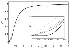
Figure 2: Ground state ALC for systems of $L=24$ (dot-dash), $40$ (dash) and $68$ (solid) levels. The bold and dotted lines show the analytic results for the thermodynamical limit and $L=2$ respectively. The inset, showing the result for small $\lambda$, highlights that the ALC is $L$-dependent and not universal.

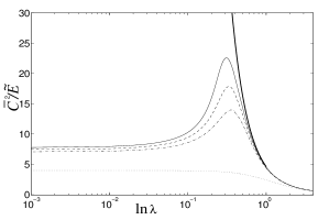
Figure 3: The ratio $\overline{C}^{2}/\tilde{E}$ versus $\ln(\lambda)$. The results shown are for $L=24$ (dot-dash), $40$ (dash) and $68$ (solid) levels, while the bold and dotted curves are the analytic results obtained for the thermodynamic limit and $L=2$. The maximum for each case is a threshold coupling, below which other EMs become significant. For $L=2$ and the thermodynamic limit the maximum occurs at $\lambda=0$, as there is only bi-partite entanglement in these cases.

To analyse the ground state ALC in the canonical case we employ results from the exact solution r . An eigenstate of (2) with $M$ Cooper pairs is characterised by a set of complex parameters $\{v_{1},\dots,v_{M}\}$ which provide a solution to the set of Bethe Ansatz Equations (BAE)

$$\frac{2}{d\lambda}+\sum_{k=1}^{L}\frac{1}{v_{i}-\epsilon_{k}} = \sum_{j\neq i}^{M}\frac{2}{v_{i}-v_{j}},$$ (8)

and the energy is given by $E=2\sum_{j=1}^{M}v_{j}+\lambda dM$. For the simple case of $L=2,\,M=1$, (8) can be solved analytically yielding the ground state energy $E=\epsilon_{1}+\epsilon_{2}-\sqrt{d^{2}\lambda^{2}+(\epsilon_{1}-\epsilon_{2})^{2}}$. Using the Hellmann-Feynman theorem the correlators (6) can be computed which gives the ALC as $\overline{C}=\lambda/{\sqrt{1+\lambda^{2}}}$.

For the case of general finite $L$ the ALC can be computed through determinant representations of the $\tilde{C}_{j}$ which are given as functions of the set $\{v_{1},\dots,v_{M}\}$. The explicit formulae can be found in zlmg ; lzmg . In the limits of weak f and strong yba coupling for large but finite $L$ we have the asymptotic results

$$\tilde{E} \sim \lambda/2(1+O(1/L)),$$

$$\overline{C} \sim 1-1/(6\lambda^{2})(1+O(1/L)),~{}~{}~{}~{}~{}~{}~{}~{}~{}~{}~{}~{}~{}~{}~{}~{}~{}\,\lambda^{-1}\ll 1,$$

$$\tilde{E} \sim \lambda^{2}\ln(2)/L(1+O(1/\ln L)),\,\,$$

$$\overline{C} \sim \lambda\sqrt{{2}/{L}}\,\ln(3+\sqrt{8})(1+O(1/\ln L)),\,\ \ \,~{}~{}~{}~{}~{}\lambda\ll 1.$$

It is found that for $\lambda^{-1}\ll 1$, $\overline{C}^{2}/\tilde{E}\sim 2/\lambda$, and   

$$\overline{C}^{2}/\tilde{E} \sim (2\ln^{2}(3+\sqrt{8}))/\ln(2)\approx 8.97$$

for $\lambda\ll 1$. Therefore in the FD and SC regimes the the quantity $\overline{C}^{2}/\tilde{E}$ displays scaling behaviour, i.e. the leading term is independent of $L$. In contrast to the FD and SC regimes, which are characterised by the scales $1/\ln(L)$ and $1/L$ respectively, the scale $1/\ln^{2}(L)$ occurs for the crossover regime f .

In Fig. 2 we show the ALC versus $\lambda$ for $L=2,\,24,\,40,\,68$ and the thermodynamic limit. Like the condensation energy, it is clear that the ALC is a smooth monotonic function of $\lambda$ as it crosses from the FD to the SC regime. In Fig. 3 we plot the ratio $\overline{C}^{2}/\tilde{E}$ versus $\ln(\lambda)$, for the finite cases $L=24,40,68$. For sufficiently small $\lambda$ this ratio is approximately the constant value 8.97 (up to a small correction $O(1/\ln(L))$) in agreement with the asymptotic result, but is nonetheless monotonically increasing. At sufficiently large $\lambda$ the ratio is monotonically decreasing and is well approximated by the analytic curve for the thermodynamic limit. For $L=2$ and the thermodynamic limit the curves, also shown, are monotonic, while in each of the other three cases there is clearly a maximum at a finite value of $\ln(\lambda)$. The coupling at which the maximum of $\overline{C}^{2}/\tilde{E}$ occurs is a threshold: below this coupling (3) no longer approximates the ground state and we must expect that other (generally multi-partite) EMs become significant.

For larger values of $L$, we appeal to a heuristic argument based on the observation made in f : for the crossover regime, the condensation energy is roughly reproduced by simply summing up the contributions from the perturbative result in the FD regime and the BCS mean field theory in the SC regime gg . This also applies to the ALC. Therefore, the same picture we have drawn from exact Bethe ansatz solutions for small $L$ works for very large $L$, thus filling in the gap between the tractable but relatively small $L$’s and the thermodynamic limit. As $L$ becomes very large, the threshold coupling tends to the value $2/\ln(L)$ (the coupling at which mean-field theory breaks down f ). This gives $\overline{C}^{2}/\tilde{E}\sim\ln^{2}(L)$ at the threshold, showing the peak in Fig. 3 is not bounded as $L$ increases. The competition of different scales in the crossover regime leads to the breakdown of the scaling behaviour observed in the FD and SC regimes.

We gratefully acknowledge financial support from the Australian Research Council.

References

- (1) S. Popescu and D. Rohrlich, Phys. Rev. A 56 R3319 (1997)
- (2) S. Hill and W.K. Wootters, Phys. Rev. Lett. 78, 5022 (1997)
- (3) Z. Gedik, Solid State Commun. 124 473 (2002)
- (4) M.A. Martín-Delgado, quant-ph/0207026
- (5) V. Coffman, J. Kundu and W.K. Wootters, Phys. Rev. A 61 052306 (2000)
- (6) R.M. Gingrich, Phys. Rev. A 65 052302 (2002)
- (7) N. Linden, S. Popescu and A. Sudbery, Phys. Rev. Lett. 83 243 (1999)
- (8) J. Kempe, Phys. Rev. A 60 910 (1999)
- (9) R.W. Richardson, Phys. Lett. 3 277 (1963); ibid 5 82 (1963)
- (10) H.-Q. Zhou, J. Links, R.H. McKenzie and M.D. Gould, Phys. Rev. B 65 060502(R) (2002)
- (11) J. Links, H.-Q. Zhou, R.H. McKenzie and M.D. Gould, J. Phys. A: Math. Gen. 36 R63 (2003)
- (12) M.R. Dowling, A.C. Doherty and S.D. Bartlett, Phys. Rev. A 70 062113 (2004)
- (13) J. Dukelsky and G. Sierra, Phys. Rev. B 61 12302 (2000)
- (14) J. von Delft and D.C. Ralph, Phys. Rep. 345 61 (2001)
- (15) P. Zanardi, Phys. Rev. A 65 042101 (2002)
- (16) P. Zanardi and X. Wang, J. Phys. A: Math. Gen. 35 7947 (2002)
- (17) L.N. Cooper, J. Bardeen and J.R. Schrieffer, Phys. Rev. 108 1175 (1957)
- (18) P.W. Anderson, Phys. Rev. 112 1900 (1958)
- (19) M. Schechter, Y. Imry, Y. Levinson and J. von Delft, Phys. Rev. B 63 214518 (2001).
- (20) E.A. Yuzbashyan, A.A. Baytin and B.L. Altshuler, Phys. Rev. B 68 214509 (2003)
- (21) Other fittings are available, see e.g. Eq. (24) in Ref. f . However, this does not affect our qualitative discussion.