Theory of multiwave mixing and decoherence control in qubit array system

Abstract

We develop a theory to analyze the decoherence effect in a charged qubit array system with photon echo signals in the multiwave mixing configuration. We present how the decoherence suppression effect by the bang-bang control with the $\pi$ pulses can be demonstrated in laboratory by using a bulk ensemble of exciton qubits and optical pulses whose pulse area is even smaller than $\pi$. Analysis is made on the time-integated multiwave mixing signals diffracted into certain phase matching directions from a bulk ensemble. Depending on the pulse interval conditions, the cross over from the decoherence acceleration regime to the decoherence suppression regime, which is a peculiar feature of the coherent interaction between a qubit and the reservoir bosons, may be observed in the time-integated multiwave mixing signals in the realistic case including inhomogeneous broadening effect. Our analysis will successfully be applied to precise estimation of the reservoir parameters from experimental data of the direction resolved signal intensities obtained in the multiwave mixing technique.

I Introduction

The analysis of decoherence of elementary excitations in solid state is one of the main approaches to understand physics in condensed matter. It also attracts much attention in device physics attempting to implement quantum information processing devices. A central issue is how to realize and control coherent evolution of well coded quantum states. Effective means should be chosen depending on the way of coupling to the system and decoherence mechanism. Among various proposals semiconductor devices have potential advantages, including the ease of integration and the use of matured industrial technologies.

In particular, excitons in semiconductor make clear distinction from other two level systems for qubits in the sense that it can efficiently couple to photons, which are the signal carriers to build a communication network. In addition, its large dipole moment makes possible direct optical control of qubits in a time scale of femto second. Various results of optical coherent manipulation of exciton in semiconductor have been reported, such as indirect Cundiff94 ; Giessen98 and direct Schulzgen99 observations of excitonic Rabi oscillations in higher dimensional semiconductor structures, manipulations of a one-qubit rotation of a single quantum dot exciton Bonadeo98 ; Toda00 ; Stievater01 ; Kamada01 ; Htoon02 , direct observations of excitonic Rabi oscillations in quantum dot ensemble Borri02 , and entanglement manipulation in quantum dots Chen00 ; Bayer01 . They open great opportunities for quantum information processing based on exciton qubits.

On the other hand, exciton qubits always suffer from unwanted coupling with the external degrees of freedom of charged excitations including the phonon scattering and the scattering by excitons themselves, leading to the decoherence. In particular, the fast decoherence time of excitons which is typically a few tens of pico second will be the first obstacle to be overcome.

The well known methods to fight the decoherence are quantum error correcting codes Shor95 ; Steane96 ; CalderbankShor96 ; Gottesman96 ; KnillLaflamme97 ; Calderbank_etal97 and encoding with decoherence free subspace PalmaSuominenEkert96 ; Zanardi97 ; Duan98 ; Lidar98 ; Knill00 ; Kempe01 ; Lidar01 . Both methods rely on encoding with multipartite entangled states for correcting errors by redundant qubits, or for making the state evolution immune to decoherence by exploiting symmetries of the system-environment interaction. It is yet very challenging to prepare the multipartite entangled states in the desired form in solid state device.

The other, and only plausible method with present technologies might be the dynamical decoupling control by driving the system continuously with external pulsed field sequences, the so called bang-bang (BB) control Ban98 ; ViolaLloyd98 ; Duan99 ; Viola99a ; Zanardi99 ; Vitali99 ; Viola99b ; Viola00 ; Vitali02 ; Byrd01 ; Cory00 ; Agarwal01 ; Uchiyama02 , or with projecting onto a certain measurement basis Facchi00 ; FacchiPascazio02 ; Nakazato03 , the so called quantum Zeno effect (for recent review, see HomeWhitaker_Rev_Q_Zeno97 ; FacchiPascazio_Rev_Q_Zeno01 ). This does not basically require complicated qubit encoding, but effective at a single qubit level. The former is easier from the technical viewpoint, and therefore to be demonstrated as the first step for solid state qubits. The BB control relies on a time reversal of the decoherece process in a short time scale within the reservoir correlation time. Similar ideas have been known such as spin echoes Hahn50 , photon echoes Kurnit64 , wave packet echoes Buchkremer00 , and charge echoes Nakamura02 ; Creswick04 . These techniques have been powerful tools to investigate transient phenomena. The BB control can be regarded as a variant of them, focusing on an active decoherence control of qubit. This has been demonstrated recently with a solid-state nulear qubit Ladd04 .

Our concern here is the BB control with optical pulses for exciton qubits in semiconductor. In order to put this method to the experimental test, we will face mainly two problems. One is the difficulty of detecting the expected stabilization effect by weak signals from a single exciton qubit. The other is that the presently available laser power is not strong enough yet for preparing the $\pi$ pulse area. One possible solution is to use a bulk ensemble of excitons. Strong signals from the ensemble make the detection easy. Furthermore they make it possible to observe the decoherence suppression effect due to the ideal $\pi$ pulses even if the irradiated pulses have the area of smaller than $\pi$. This is because some fraction of qubits can effectively feel the ideal $\pi$ pulses, and they form a macroscopic polarization lattice which radiates photon echo signals in a certain phase matching direction. The bulk ensemble is, however, always associated with irrelevant phenomena to the present issue, such as inhomogeneous broadening of the energy levels and complicated light diffraction due to polarization lattices of excitons.

It is then necessary to extend the theories for a single qubit to a qubit array system to analyze the effect of our interest with rather complicated signals. The purpose of this paper is to develop a theory to analyze the decoherence with the photon echo signals in the multiwave mixing configuration, and to predict the effects of decoherence control in a practical experimental setting.

The paper is organized as follows. In section II we present the model and introduce basic notations. In section III we first develop a formulation to evaluate the multiwave mixing signals in the ideal $\pi$ pulse case. We then present the results in the case of homogeneous broadening, and introduce basic notions to analyze the state evolution of the qubit-reservoir system using the multiwave mixing signals. In section IV we develop a formulation for the weak pulse case, and present numerical simulations on the time-resolved and time-integated multiwave mixing signals. They include not only the suppression but also the acceleration of decoherence induced by the optical BB control. Section V is for concluding remark.

II Model

In this paper we consider an ensemble of qubits and identical reservoirs. The model Hamiltonian is given by

$$\hat{H}(t)=\hat{H}_{0}+\hat{H}_{\rm QR}+\hat{H}_{\rm QF}(t),$$ (1)

where

$$\hat{H}_{0}=\sum_{j}\left[{1\over 2}\hbar\nu_{j}\hat{\sigma}_{z}(j)+\sum_{l}\hbar\Omega_{l}\hat{B}^{\dagger}_{l}(j)\hat{B}_{l}(j)\right],$$ (2)

$$\hat{H}_{\rm QR}=\sum_{j}\hbar\hat{\sigma}_{z}(j)\sum_{l}\left[g_{l}\hat{B}^{\dagger}_{l}(j)+g^{\ast}_{l}\hat{B}_{l}(j)\right],$$ (3)

$$\hat{H}_{\rm QF}(t)=\sum_{j}\hbar\kappa\hat{\sigma}_{+}(j)\sum_{m}E_{m}(t){\rm e}^{i[\mathbf{k}_{m}\cdot\mathbf{r}_{j}-\omega t]}+\rm{c.c}.$$ (4)

$\hat{H}_{0}$ describes the free evolution of the qubit and the reservoir systems. The index $j$ refers to the $j$th site of qubit whose ground and excited states are $|\downarrow\rangle_{j}$ and $|\uparrow\rangle_{j}$, respectively. $\nu_{j}$ is the energy separation of the $j$th qubit. $\hat{\sigma}_{z}$ is the Pauli $z$ component operator. We assume that the qubit at the $j$th site interacts with its own reservoir around the site, and that the reservoirs at different sites are independent but have an identical mode structure $\{\Omega_{l}\}$ and a temperature $T$. The index $l$ is the $l$th mode of the reservoir boson with the angular frequency $\Omega_{l}$ which is described by the creation and annihilation operators $\hat{B}^{\dagger}_{l}(j)$ and $\hat{B}_{l}(j)$. $\hat{H}_{\rm QR}$ describes the coupling between the qubit and the reservoir systems by the coupling constant $g_{l}$. $\hat{H}_{\rm QF}(t)$ describes the qubit-external field interaction in the rotating wave approximation. $\kappa$ is its coupling constant. $\hat{\sigma}_{+}(j)$ acts as $\hat{\sigma}_{+}(j)|\downarrow\rangle_{j}=|\uparrow\rangle_{j}$. $\mathbf{r}_{j}$ is the coordinate of the $j$th site of qubit. $E_{m}(t)$, $\mathbf{k}_{m}$, and $\omega$ are the external (classical) field amplitude, its wave vector, and angular frequency of the $m$th pulse.

The essential physics of the decoherence in the above model is the same as that in the model consisting of a single qubit and a bosonic thermal reservoir, and has already been clarified by extensive theoretical analyses PalmaSuominenEkert96 ; ViolaLloyd98 ; Ban98 ; Uchiyama02 . The new feature included in the above model is just an array structure of qubits. Main concern here is to know how the decoherence occuring at a single qubit level can be detected in the multiwave mixing signals from this array structure.

The interaction pictured Hamiltonians are given by

$$\tilde{H}_{\rm QR}(t)=\sum_{j}\hbar\hat{\sigma}_{z}(j)\sum_{l}\left[g_{l}\hat{B}^{\dagger}_{l}(j){\rm e}^{i\Omega_{l}t}+g^{\ast}_{l}\hat{B}_{l}(j){\rm e}^{-i\Omega_{l}t}\right],$$ (5)

$$\tilde{H}_{\rm QF}(t)=\sum_{j}\hbar\kappa\hat{\sigma}_{+}(j)\sum_{m}E_{m}(t){\rm e}^{i[\mathbf{k}_{m}\cdot\mathbf{r}_{j}+(\nu_{j}-\omega)t]}+\rm{h.c}.$$ (6)

For simplicity, we assume that the optical field in $\tilde{H}_{\rm QF}(t)$ are composed of a sequence of optical pulses with rectangular temporal shape as shown in Fig. 1 which are specified by

$$E_{m}(t)=\biggl{\{}\begin{array}[]{ll}{\bar{E}}_{m}&(t_{m}\leq t\leq t_{m}+\tau_{m})\\ 0&{\rm otherwise}\end{array}.$$ (7)

We further assume that the pulse duration $\tau_{m}$ is so short that the effect of the qubit-reservoir interaction $\tilde{H}_{\rm QR}(t)$ can be neglected during the period $[t_{m},t_{m}+\tau_{m}]$. Taking the limit of $\tau_{m}\rightarrow 0$ and $\bar{E}_{m}\rightarrow\infty$ with the finite pulse area ${\theta_{m}}=-2i{\bar{E}}_{m}\tau_{m}\kappa$, the state evolution under the $m$th optical pulse is described by the unitary operator

$$\tilde{U}^{(m)}_{\rm QF}=\prod_{j}\tilde{u}^{(m)}_{\mathrm{QF}j}$$ (8)

with

$$\tilde{u}^{(m)}_{\mathrm{QF}j}=\mathrm{exp}\left\{{\theta_{m}\over 2}\left[\hat{\sigma}_{+}(j)\mathrm{e}^{i\phi^{(m)}_{j}}-\hat{\sigma}_{-}(j)\mathrm{e}^{-i\phi^{(m)}_{j}}\right]\right\},$$ (9)

where $\phi^{(m)}_{j}=\mathbf{k}_{m}\cdot\mathbf{r}_{j}+(\nu_{j}-\omega)t_{m}$. Each qubit evolves according to

$$\tilde{u}^{(m)}_{\mathrm{QF}j}|\downarrow\rangle_{j}=\mathrm{cos}{\theta_{m}\over 2}|\downarrow\rangle_{j}+\mathrm{e}^{i\phi^{(m)}_{j}}\mathrm{sin}{\theta_{m}\over 2}|\uparrow\rangle_{j},$$ (10)

$$\tilde{u}^{(m)}_{\mathrm{QF}j}|\uparrow\rangle_{j}=\mathrm{cos}{\theta_{m}\over 2}|\uparrow\rangle_{j}-\mathrm{e}^{-i\phi^{(m)}_{j}}\mathrm{sin}{\theta_{m}\over 2}|\downarrow\rangle_{j}.$$ (11)

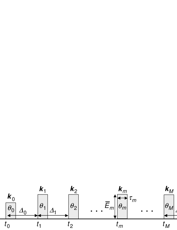
Figure 1: Optical pulse sequence.

The state evolution between the pulses are described by the qubit-reservoir interaction

$$\tilde{U}^{(m)}_{\mathrm{QR}} = T{\rm exp}\left[-{i\over\hbar}\int_{t_{m}}^{t_{m+1}}dt^{\prime}\tilde{H}_{\rm QR}(t^{\prime})\right]$$ (12)

$$= \prod_{j}\tilde{u}^{(m)}_{\mathrm{QR}j},$$ (13)

with

$$\tilde{u}^{(m)}_{\mathrm{QR}j}=\mathrm{exp}\left[i\Theta(t_{m+1},t_{m})+\hat{\sigma}_{z}(j)\sum_{l}\left(\alpha^{(m)}_{l}\hat{B}^{\dagger}_{l}(j)-\alpha^{(m)\ast}_{l}\hat{B}_{l}(j)\right)\right],$$ (14)

where

$$\Theta(t_{m+1},t_{m})=\sum_{l}|g_{l}|^{2}\frac{\Omega_{l}(t_{m+1}-t_{m})-\mathrm{sin}\left[\Omega_{l}(t_{m+1}-t_{m})\right]}{\Omega_{l}^{2}},$$ (15)

and

$$\alpha^{(m)}_{l}={g_{l}\over\Omega_{l}}\left[\mathrm{e}^{i\Omega_{l}t_{m}}-\mathrm{e}^{i\Omega_{l}t_{m+1}}\right].$$ (16)

To evaluate the state evolution by $\tilde{U}^{(m)}_{\mathrm{QR}}$, we may use the formula

$$\tilde{u}^{(m)}_{\mathrm{QR}j}|\downarrow\rangle_{j}\otimes|\Psi\rangle_{\mathrm{R}j}=|\downarrow\rangle_{j}\otimes\hat{D}^{(m)}_{j-}|\Psi\rangle_{\mathrm{R}j},$$ (17)

$$\tilde{u}^{(m)}_{\mathrm{QR}j}|\uparrow\rangle_{j}\otimes|\Psi\rangle_{\mathrm{R}j}=|\uparrow\rangle_{j}\otimes\hat{D}^{(m)}_{j+}|\Psi\rangle_{\mathrm{R}j},$$ (18)

where the state $|\Psi\rangle_{\mathrm{R}j}$ represents any pure state component of the $j$th reservoir and

$$\hat{D}^{(m)}_{j\pm}\equiv\prod_{l}\hat{D}_{j}(\pm\alpha^{(m)}_{l})$$ (19)

with the displacement operators

$$\hat{D}_{j}(\pm\alpha^{(m)}_{l})=\mathrm{exp}\left(\pm\alpha^{(m)}_{l}\hat{B}^{\dagger}_{l}(j)\mp\alpha^{(m)\ast}_{l}\hat{B}_{l}(j)\right).$$ (20)

For the state $|\Psi\rangle_{\mathrm{R}j}$, we will later substitute the Fock state basis $|n_{1}...n_{l}...\rangle_{j}$ which describes the occupation of the reservoir boson modes.

The total evolution operator for the $M$ pulse sequence is given by

$$\tilde{U}(t,t_{0})=\prod_{j}\tilde{u}_{j}(t,t_{0}),$$ (21)

with

$$\tilde{u}_{j}(t,t_{0})=\tilde{u}^{(M)}_{\mathrm{QR}j}\tilde{u}^{(M)}_{\mathrm{QF}j}\cdot\tilde{u}^{(M-1)}_{\mathrm{QR}j}\tilde{u}^{(M-1)}_{\mathrm{QF}j}\cdots\tilde{u}^{(1)}_{\mathrm{QR}j}\tilde{u}^{(1)}_{\mathrm{QF}j}\tilde{u}^{(0)}_{\mathrm{QR}j}\tilde{u}^{(0)}_{\mathrm{QF}j}.$$ (22)

As for $\tilde{u}^{(M)}_{\mathrm{QR}j}$, we use

$$\alpha^{(M)}_{l}={g_{l}\over\Omega_{l}}\left[\mathrm{e}^{i\Omega_{l}t_{M}}-\mathrm{e}^{i\Omega_{l}t}\right],$$ (23)

i.e., $t_{M+1}$ is understood as $t$, instead of the definition of Eq. (16). The final state of the total system is represented by

$$\tilde{\rho}_{\rm QR}(t)=\tilde{U}(t,t_{0})\tilde{\rho}_{\rm QR}(t_{0})\tilde{U}(t,t_{0})^{\dagger},$$ (24)

where we assume the initial state like

$$\tilde{\rho}_{\rm QR}(t_{0})=\prod_{j}|\downarrow\rangle_{j}\langle\downarrow|\otimes\prod_{l}\hat{\rho}_{{\rm R}j,l}(T)$$ (25)

with the thermal state

$$\hat{\rho}_{{\rm R}j,l}(T) = (1-{\rm e}^{-\hbar\Omega_{l}/k_{\rm B}T}){\rm e}^{-\hbar\Omega_{l}\hat{B}^{\dagger}_{l}(j)\hat{B}_{l}(j)/k_{\rm B}T},$$ (26)

$$= \sum_{n_{l}(j)=0}^{\infty}\frac{\bar{n}_{l}^{n_{l}(j)}}{(1+\bar{n}_{l})^{n_{l}(j)+1}}|n_{l}(j)\rangle_{\mathrm{R}j}\langle n_{l}(j)|,$$ (27)

where

$$\bar{n}_{l}=1/\left(\mathrm{e}^{\hbar\Omega_{l}/k_{\rm B}T}-1\right).$$ (28)

By using the formula Eqs. (17) and (18), the final state can be represented as

$$\tilde{\rho}_{\rm QR}(t)=\prod_{j}\left[\sum_{\vec{n}(j)}\left(\prod_{l=1}^{\infty}\frac{\bar{n}_{l}^{n_{l}(j)}}{(1+\bar{n}_{l})^{n_{l}(j)+1}}\right)|\tilde{\rho}_{\vec{n}(j)}(t)\rangle_{{\rm QR}j}\langle\tilde{\rho}_{\vec{n}(j)}(t)|\right],$$ (29)

where

$$|\tilde{\rho}_{\vec{n}(j)}(t)\rangle_{{\rm QR}j}\equiv\tilde{u}_{j}(t,t_{0})|\downarrow\rangle_{j}\otimes|\vec{n}(j)\rangle_{\mathrm{R}j},$$ (30)

and $\vec{n}(j)\equiv(n_{0}(j),...,n_{l}(j),...)$ denoting the boson number occupation. To describe the state of Eq. (30), we introduce the two operators $\hat{F}^{(M)}_{j}$ and $\hat{G}^{(M)}_{j}$ by

$$|\tilde{\rho}_{\vec{n}(j)}(t)\rangle_{{\mathrm{Q}R}j}\equiv(-1)^{M\over 2}\biggl{(}|\downarrow\rangle_{j}\otimes\hat{G}^{(M)}_{j}+|\uparrow\rangle_{j}\otimes\hat{F}^{(M)}_{j}\biggr{)}|\vec{n}(j)\rangle_{{\mathrm{R}}j},$$ (31)

for $M=$even, and

$$|\tilde{\rho}_{\vec{n}(j)}(t)\rangle_{{\mathrm{Q}R}j}\equiv(-1)^{{M-1}\over 2}\biggl{(}-|\downarrow\rangle_{j}\otimes\hat{F}^{(M)}_{j}+|\uparrow\rangle_{j}\otimes\hat{G}^{(M)}_{j}\biggr{)}|\vec{n}(j)\rangle_{{\mathrm{R}}j},$$ (32)

for $M=$odd.

III State evolution under $\pi$ pulses

III.1 Formulation

In this section we consider the pulse sequence consisting of the 0th exciting pulse with the area $\theta_{0}=\pi/2$ at time $t_{0}$, and the subsequent $M$ $\pi$-pulses, i.e., $\theta_{m}=\pi$ $(m=1,...,M)$. By using Eqs. (10), (11), (17), and (18), we obtain

$$\hat{F}^{(M)}_{j}={1\over{\sqrt{2}}}\mathrm{e}^{i(\Phi^{(M)}_{j}+\phi^{(0)}_{j})}\hat{D}^{(M)}_{j(-1)^{M}}\cdots\hat{D}^{(1)}_{j-}\hat{D}^{(0)}_{j+}$$ (33)

and

$$\hat{G}^{(M)}_{j}={1\over{\sqrt{2}}}\mathrm{e}^{-i\Phi^{(M)}_{j}}\hat{D}^{(M)}_{j(-1)^{M+1}}\cdots\hat{D}^{(1)}_{j+}\hat{D}^{(0)}_{j-}$$ (34)

where

$$\Phi^{(M)}_{j}=\sum_{m=1}^{M}(-1)^{m}\phi^{(m)}_{j}.$$ (35)

The decoherence property of the qubit system is measured by observing the intensity of the radiation from the macroscopic polarization. The polarization operators in the interaction picture are defined by

$$\tilde{S}_{\pm}(\mathbf{q},t)\equiv\sum_{j}\hat{\sigma}_{\pm}(j)\mathrm{e}^{i\mathbf{q}\cdot\mathbf{r}_{j}\pm\nu_{j}t}.$$ (36)

The macroscopic polarization is then evaluated by

$$P(\mathbf{q},t) = {\rm Tr}\left[\sum_{j}\tilde{S}_{+}(\mathbf{q},t)\tilde{\rho}_{\rm QR}(t)\right]\mathrm{e}^{-i\omega t},$$ (41)

$$= \sum_{j}{\rm e}^{i[\mathbf{q}\cdot\mathbf{r}_{j}+(\nu_{j}-\omega)t]}{\rm Tr}\left[\tilde{\sigma}_{+}(j)\tilde{\rho}_{\rm QR}(t)\right],$$

$$= \Biggl{\{}\begin{array}[]{lll}{}&\displaystyle\sum_{j}{\rm e}^{i[\mathbf{q}\cdot\mathbf{r}_{j}+(\nu_{j}-\omega)t]}{\rm Tr}_{\rm R}\left[\hat{F}^{(M)\dagger}_{j}\hat{G}^{(M)}_{j}\prod_{l}\hat{\rho}_{{\rm R}j,l}(T)\right],&(M={\rm even}),\\ {}&{}&{}\\ -&\displaystyle\sum_{j}{\rm e}^{i[\mathbf{q}\cdot\mathbf{r}_{j}+(\nu_{j}-\omega)t]}{\rm Tr}_{\rm R}\left[\hat{G}^{(M)\dagger}_{j}\hat{F}^{(M)}_{j}\prod_{l}\hat{\rho}_{{\rm R}j,l}(T)\right],&(M={\rm odd}),\end{array}$$

$$= \frac{(-1)^{M}}{2}\sum_{j}{\rm exp}i\left[\mathbf{q}\cdot\mathbf{r}_{j}+(\nu_{j}-\omega)t+(-1)^{M+1}\left(2\Phi_{j}^{(M)}+\phi_{j}^{(0)}\right)\right]$$

$$\times{\rm Tr}_{\rm R}\left[\prod_{l}\hat{D}_{j}\left((-1)^{M+1}2\sum_{m=0}^{M}(-1)^{m}\alpha_{l}^{(m)}\right)\hat{\rho}_{{\rm R}j,l}(T)\right],$$

Let us introduce the decoherence exponent by

$${\rm e}^{-\Gamma(t)}\equiv{\rm Tr}_{\rm R}\left[\prod_{l}\hat{D}_{j}\left((-1)^{M+1}2\sum_{m=0}^{M}(-1)^{m}\alpha_{l}^{(m)}\right)\hat{\rho}_{{\rm R}j,l}(T)\right].$$ (42)

The decoherence exponent, which is now independent of $j$, is expressed as PalmaSuominenEkert96 ; ViolaLloyd98

$$\Gamma(t) = {1\over 2}\sum_{l}\Biggl{|}2\sum_{m=0}^{M}(-1)^{m}\alpha_{l}^{(m)}\Biggr{|}^{2}\mathrm{coth}\left(\frac{\hbar\Omega_{l}}{2k_{\mathrm{B}}T}\right)$$ (43)

$$= 2\sum_{l}\frac{|g_{l}|^{2}}{\Omega^{2}_{l}}f(\Omega_{l},t)\mathrm{coth}\left(\frac{\hbar\Omega_{l}}{2k_{\mathrm{B}}T}\right),$$

$$= 2\int_{0}^{\infty}d\Omega I(\Omega)\frac{f(\Omega,t)}{\Omega^{2}}\mathrm{coth}\left(\frac{\hbar\Omega}{2k_{\mathrm{B}}T}\right),$$

where

$$I(\Omega)=\sum_{l}\delta(\Omega-\Omega_{l})|g_{l}|^{2},$$ (44)

and

$$f(\Omega,t)=\left|\sum_{m=0}^{M-1}(-1)^{m}({\rm e}^{i\Omega t_{m}}-{\rm e}^{i\Omega t_{m+1}})+(-1)^{M}({\rm e}^{i\Omega t_{M}}-{\rm e}^{i\Omega t})\right|^{2}.$$ (45)

By substituting the definition of $\Phi_{j}^{(M)}$ (Eq. (35)) and $\phi^{(m)}_{j}=\mathbf{k}_{m}\cdot\mathbf{r}_{j}+(\nu_{j}-\omega)t_{m}$ into Eq. (41), we have

$$P(\mathbf{q},t)=\frac{(-1)^{M}}{2}{\rm e}^{-\Gamma(t)}\sum_{j}{\rm exp}i\left[\left(\mathbf{q}-(-1)^{M}\mathbf{K}^{(M)}\right)\cdot\mathbf{r}_{j}+(\nu_{j}-\omega)\left(\Delta_{M}+(-1)^{M}\sum_{m=0}^{M-1}(-1)^{m}\Delta_{m}\right)\right],$$ (46)

where

$$\mathbf{K}^{(M)}=2\sum_{m=1}^{M}(-1)^{m}\mathbf{k}_{m}+\mathbf{k}_{0},$$ (47)

$\Delta_{m}\equiv t_{m+1}-t_{m}$, and $\Delta_{M}\equiv t-t_{M}$. Eq. (46) shows that the radiation signal is observed in the phase matching direction $\mathbf{q}=(-1)^{M}\mathbf{K}^{(M)}$.

III.2 Homogeneous case

We first consider the homogeneous case of $\nu=\nu_{i}$ for all $i$. This case was already studied by Aihara as the photon echo in the four wave mixing (two pulse) scheme Aihara80 ; Aihara82 . He pointed out that the interaction between the qubit and the reservoir bosons induces the slow frequency modulation on the qubit in the short time region where the reservoir keeps the phase memory, and plays the similar role to the inhomogeneous broadening. In fact he predicted that the photon echo must be observed even in the homogeneous case. The BB control proposed by Ban Ban98 , and Viola and Lloyd ViolaLloyd98 can be regarded as a natural extension of this principle to the multi-pulse scheme. It is well studied how to design a pulse sequence for effective suppression of decoherence Ban98 ; ViolaLloyd98 ; Uchiyama02 . The decoherence can be made worse by applying a pulse sequence, if the pulse intervals are not taken short enough.

Figure 2: The time-resolved multiwave mixing signal intensities under the multi $\pi$ pulse irradiation (solid lines) compared with the ones of the free induction decay (one dotted lines) in the case of the ohmic reservoir model. The parameters are $\Omega_{\rm c}$=8 meV, $\alpha=0.1$ and $T$=10 K. $M$ is the number of pulses and $\Delta$ is the pulse interval.

Figure 3: The time-resolved multiwave mixing signal intensities under the multi $\pi$ pulse irradiation (solid lines) compared with the ones of the free induction decay (one dotted lines) in the case of the Gaussian-ohmic reservoir model. The parameters are $\Omega_{\rm p}$=13 meV, $\gamma_{\rm p}$=4 meV, $\alpha_{\rm p}=0.05$, $\Omega_{\rm c}$=8 meV, $\alpha=0.1$, and $T$=10 K. $M$ is the number of pulses and $\Delta$ is the pulse interval.

Fig. 2 shows numerical results of the decoherence under an $M$ $\pi$ pulse sequence with an interval $\Delta$. The solid lines represent the time-resolved multiwave mixing signal intensities of the multiwave mixing signals, $I_{\mathbf{q}}(t)=|P(\mathbf{q},t)|^{2}$, in the phase matching direction $\mathbf{q}=(-1)^{M}\mathbf{K}^{(M)}$ (Eq. (47)), while the one dotted lines represent the ones of the free induction decay signals in the direction $\mathbf{k}_{0}$. We have assumed the ohmic reservoir model characterized by the spectral density

$$I(\Omega)=\alpha\Omega{\rm exp}(-\frac{\Omega}{\Omega_{\rm c}}),$$ (48)

where $\Omega_{\rm c}$ is the cutoff frequency and $\alpha$ is the dimensionless coupling constant. As seen, for a pulse interval of $\Delta=0.2$ ps, the decoherece is not suppressed but accelerated. In Fig. 3, we have shown the same kind of results in the case of the Gaussian-ohmic reservoir model, which has not only the ohmic character with a wider spectrum but also the Gaussian character with a sharper spectrum around a characteristic frequency $\Omega_{\rm p}$, such as a specific phonon mode. The decay profile exhibits the oscillation characterized by the frequency $\Omega_{\rm p}$. For shorter pulse intervals, the decoherence is accelerated by adding $\pi$ pulses.

$$I(\Omega)=\alpha\Omega{\rm exp}(-\frac{\Omega}{\Omega_{\rm c}})+\frac{\alpha_{\rm p}\Omega^{2}}{\sqrt{\pi}\gamma_{\mathrm{p}}}{\rm exp}\left[-\frac{(\Omega-\Omega_{\mathrm{p}})^{2}}{\gamma_{\mathrm{p}}^{2}}\right].$$ (49)

Although this decoherence acceleration phenomenon is essential to understand the decoherence, its interpretation given so far is unsatisfactory. Here we revisit this point by considering a simplified model

$$\hat{H}_{{\rm QR}_{\rm S}}(t)=\hbar\hat{\sigma}_{z}(g_{\mathrm{p}}\hat{B}^{\dagger}+g^{\ast}_{\mathrm{p}}\hat{B}),$$ (50)

i.e., a signal qubit interacts with a single mode field of the reservoir boson oscillator with the angular frequency $\Omega_{\mathrm{p}}$. Under this Hamiltonian, the qubit couples with the reservoir as

$$(|\uparrow\rangle+|\downarrow\rangle)\otimes|n\rangle_{\rm R}$$ (51)

$$\rightarrow \left(|\uparrow\rangle\otimes\hat{D}[\alpha(t-t_{0})]+|\downarrow\rangle\otimes\hat{D}[-\alpha(t-t_{0})]\right)|n\rangle_{\rm R},$$

where $|n\rangle_{\rm R}$ is the n boson state component, and

$$\hat{D}\left(\pm\alpha(t-t_{0})\right)=\mathrm{exp}\left[\pm\alpha(t-t_{0})\hat{B}^{\dagger}\mp\alpha(t-t_{0})^{\ast}\hat{B}\right],$$ (52)

with

$$\alpha(t-t_{0})=\frac{g_{\mathrm{p}}}{\Omega_{\mathrm{p}}}({\rm e}^{i\Omega_{\mathrm{p}}t_{0}}-{\rm e}^{i\Omega_{\mathrm{p}}t}).$$ (53)

The free induction decay is characterized by the decoherence exponent

$$\Gamma_{+}(t)=2\frac{|g_{\mathrm{p}}|^{2}}{\Omega^{2}_{\mathrm{p}}}f_{+}(t)\mathrm{coth}\left(\frac{\hbar\Omega_{\mathrm{p}}}{2k_{\mathrm{B}}T}\right)\equiv g^{\prime}f_{+}(t),$$ (54)

where

$$f_{+}(t) = |{\rm e}^{i\Omega_{\mathrm{p}}t_{0}}-{\rm e}^{i\Omega_{\mathrm{p}}t}|^{2}$$ (55)

$$= 2\Biggl{\{}1-\mathrm{cos}\Bigl{[}\Omega_{\mathrm{p}}(t-t_{0})\Bigr{]}\Biggr{\}}.$$

Thus $\Gamma_{+}(t)$ oscillates in time and the qubit is recohered, i.e., disentangled from the reservoir, at $t-t_{0}=(2\pi/\Omega_{\mathrm{p}})\times$(integer). On the other hand, when a $\pi$ pulse is applied at a time $t_{1}$, the decoherence exponent is given by

$$\Gamma_{-}(t)\equiv g^{\prime}f_{-}(t)$$ (56)

with

$$f_{-}(t) = |{\rm e}^{i\Omega_{\mathrm{p}}t_{0}}-{\rm e}^{i\Omega_{\mathrm{p}}t_{1}}-({\rm e}^{i\Omega_{\mathrm{p}}t_{1}}-{\rm e}^{i\Omega_{\mathrm{p}}t})|^{2},$$ (57)

$$= 2\bigl{[}3-2\mathrm{cos}(\Omega_{\mathrm{p}}\Delta_{0})\bigr{]}$$

$$- 2\sqrt{5-4\mathrm{cos}(\Omega_{\mathrm{p}}\Delta_{0})}\mathrm{cos}[\Omega_{\mathrm{p}}(t-t_{0})+\varphi],$$

where

$$\mathrm{tan}\varphi=\frac{2\mathrm{cos}\Omega_{\mathrm{p}}\Delta_{0}}{1-2\mathrm{cos}\Omega_{\mathrm{p}}\Delta_{0}}.$$ (58)

For small enough $\Delta_{0}$ $(\equiv t_{1}-t_{0})$,

$$\Gamma_{-}(t)\sim 2g^{\prime}\left\{1-\mathrm{cos}\left[\Omega_{\mathrm{p}}(t-t_{0}-2\Delta_{0})\right]\right\}.$$ (59)

This should be compared with $\Gamma_{+}(t)$. We can see that the dephasing exponent $\Gamma_{-}(t)$ is the one shifted in time by $2\Delta_{0}$ from $\Gamma_{+}(t)$. Namely, by applying the $\pi$ pulse soon after the state $|\uparrow\rangle+|\downarrow\rangle$ is prepared, the decoherence starts to take place at the time $2\Delta_{0}$ later compared to the free induction decay without any $\pi$ pulse. For larger $\Delta_{0}$, however, this is not true. As an extreme case, we take $\Omega_{\mathrm{p}}\Delta_{0}=\pi$. Then

$$\Gamma_{-}(t)=g^{\prime}\left\{6\mathrm{cos}\left[\Omega_{\mathrm{p}}(t-t_{0})\right]+10\right\}\geq\Gamma_{+}(t).$$ (60)

In this case, the $\pi$ pulse plays a role to accelerate the decoherence. The reason is clear from the structure of $f_{-}(t)$. When the $\pi$ pulse is applied after $t_{1}-t_{0}>\pi/(2\Omega_{\mathrm{p}})$, the two successive displacement operations in the state component

$$\left(|\uparrow\rangle\otimes\hat{D}[\alpha(t-t_{1})]\hat{D}[-\alpha(t_{1}-t_{0})]-|\downarrow\rangle\otimes\hat{D}[-\alpha(t-t_{1})]\hat{D}[\alpha(t_{1}-t_{0})]\right)|n\rangle_{\rm R},$$ (61)

act as in-phase in the sense that the displacements by the amount of $\alpha(t-t_{1})$ and $-\alpha(t_{1}-t_{0})$ do not cancel out but are added in the same sign, leading to large degree of entanglement between the qubit and the reservoir. On the other hand, when no $\pi$ pulse is applied, the state evolves as

$$\left(|\uparrow\rangle\otimes\hat{D}[\alpha(t-t_{1})]\hat{D}[\alpha(t_{1}-t_{0})]+|\downarrow\rangle\otimes\hat{D}[-\alpha(t-t_{1})]\hat{D}[-\alpha(t_{1}-t_{0})]\right)|n\rangle_{\rm R},$$ (62)

where the two displacement operations act as out-of-phase, i.e., $\alpha(t-t_{1})$ and $\alpha(t_{1}-t_{0})$ nearly cancel out for $t_{1}-t_{0}>\pi/(2\Omega_{\mathrm{p}})$, leading to the recoherence of the qubit superposition state.

In a realistic thermal reservoir with many modes, the above feature is more or less smeared out, but can still be identified at low temperatures. Roughly speaking, we had better to take the $\pi$ pulse interval as

$$\Delta<\pi/(2\Omega_{\mathrm{th}}),$$ (63)

where $\Omega_{\mathrm{th}}$ is the largest characteristic frequency of the thermalized reservoir boson spectrum $I(\Omega){\rm coth}(\frac{\hbar\Omega}{2k_{\rm B}T}).$ At low temperatures, $\Omega_{\mathrm{th}}$ is roughly $\Omega_{\mathrm{c}}$ in the ohmic reservoir model (Fig. 2), or $\Omega_{\mathrm{p}}$ in the Gaussian-ohmic reservoir model (Fig. 3).

III.3 Inhomogeneous case

Figure 4: The time-resolved multiwave mixing signal intensities under the multi $\pi$ pulse irradiation (solid lines) compared with the ones of the single $\pi$ pulse, i.e., $M=1$ (one dotted lines) in the case of the ohmic reservoir model when the inhomogeneous broadening effect is taken into account by setting $\delta_{\rm B}$=5meV. The other parameters are the same as in Fig. 2.

Figure 5: The time-resolved multiwave mixing signal intensities under the multi $\pi$ pulse irradiation (solid lines) compared with the ones of the single $\pi$ pulse, i.e., $M=1$ (one dotted lines) in the case of the Gaussian-ohmic resevoir model when the inhomogeneous broadening effect is taken into account by setting $\delta_{\rm B}$=5meV. The other parameters are the same as in Fig. 3.

In this subsection we take into account the inhomogeneous broadening effect in a bulk ensemble of qubits. Now we assume that the inhomogeneous broadening of $\nu_{j}$ obeys the Gaussian distribution around the angular frequency $\omega$ of the external field

$$p(\nu-\omega)=\frac{1}{\sqrt{2\pi\delta_{\mathrm{B}}^{2}}}\mathrm{exp}\left[-\frac{(\nu-\omega)^{2}}{2\delta_{\mathrm{B}}^{2}}\right],$$ (64)

which leads us to

$$\sum_{j}{\rm exp}\left[i(\nu_{j}-\omega)\left(\Delta_{M}+(-1)^{M}\sum_{m=0}^{M-1}(-1)^{m}\Delta_{m}\right)\right]$$

$$=\int_{-\infty}^{\infty}d\nu p(\nu-\omega){\rm exp}\left[i(\nu-\omega)\left(\Delta_{M}+(-1)^{M}\sum_{m=0}^{M-1}(-1)^{m}\Delta_{m}\right)\right]$$

$$={\rm exp}\left[-{1\over 2}\left(\Delta_{M}+(-1)^{M}\sum_{m=0}^{M-1}(-1)^{m}\Delta_{m}\right)\delta_{\mathrm{B}}^{2}\right].$$ (65)

The time-resolved multiwave mixing signal intensity is finally obtained as

$$I_{(-1)^{M}\mathbf{K}^{(M)}}(t) = \Bigl{|}P\bigl{(}(-1)^{M}\mathbf{K}^{(M)},t\bigr{)}\Bigr{|}^{2}$$ (66)

$$= {1\over 4}{\rm exp}\left[-2\Gamma(t)-\left(\Delta_{M}+(-1)^{M}\sum_{m=0}^{M-1}(-1)^{m}\Delta_{m}\right)\delta_{\mathrm{B}}^{2}\right].$$

The decoherence property is evaluated by measuring the echo signal. In order to see the echo signal, we consider a pulse sequence consisting of odd number of $M$ $\pi$ pulses such as $\Delta_{0}=\Delta_{1}=...=\Delta_{M-2}\equiv\Delta$, and the last interval $\Delta_{M-1}$ $(=t_{M}-t_{M-1})$ being varied. The echo signal is then expected around $t=t_{M}+\Delta_{M-1}$ as seen from Eq. (66).

Figs. 4 and 5 shows how the results of Figs. 2 and 3 are modified, respectively, when the inhomogeneous broadening effect is taken into account. We assume $\delta_{\rm B}$=5meV. We see essentially the same behaviors as in Figs. 2 and 3 except that the echo signals are more sharpened by the fast dephasing due to the inhomogeneity. The one dotted lines correspond to the case of the single $\pi$ pulse ($M=1$), i.e., an ordinary four wave mixing scheme for photon echo experiment.

IV State evolution under weak pulses

IV.1 Formulation

In an actual optical experiment, it is often the case that the maximum laser power falls short of the ideal $\pi$ pulse and then the decoherence suppression does not work perfectly. In the qubit array system, only some fraction of qubits can be suppressed. In fact, the intensity of the multiwave mixing signal observed in the direction $(-1)^{M}\mathbf{K}^{(M)}$ will be reduced by a factor ${\rm sin}^{4}{\theta_{1}\over 2}\cdots{\rm sin}^{4}{\theta_{M}\over 2}$. In other words at least this fraction of the qubits can feel the ideal $\pi$ pulses, and their decoherence will be suppressed. From this point of view, we consider how one can demonstrate experimentally the principle of the BB control.

In the case of weak pulses, the analysis is no more straightforward. We have the complicated diffraction patterns in various directions. For simplicity, let us consider the three-pulse case consisting the 0th exciting pulse, the 1st and 2nd controlling pulses. The $\hat{F}^{(M)}_{j}$ and $\hat{G}^{(M)}_{j}$ operators are given by

$$\hat{F}^{(2)\dagger}_{j} = \mathrm{e}^{-i\phi^{(0)}_{j}}\mathrm{sin}{\theta_{0}\over 2}\mathrm{cos}{\theta_{1}\over 2}\mathrm{cos}{\theta_{2}\over 2}\hat{D}^{(2)}_{j-}\hat{D}^{(1)}_{j-}\hat{D}^{(0)}_{j-}\mathrm{e}^{i[-\alpha_{+}^{(210)}-\alpha^{(10)}]}$$ (67)

$$+ \mathrm{e}^{-i\phi^{(1)}_{j}}\mathrm{cos}{\theta_{0}\over 2}\mathrm{sin}{\theta_{1}\over 2}\mathrm{cos}{\theta_{2}\over 2}\hat{D}^{(2)}_{j-}\hat{D}^{(1)}_{j-}\hat{D}^{(0)}_{j+}\mathrm{e}^{i[-\alpha_{-}^{(210)}+\alpha^{(10)}]}$$

$$+ \mathrm{e}^{-i\phi^{(2)}_{j}}\mathrm{cos}{\theta_{0}\over 2}\mathrm{cos}{\theta_{1}\over 2}\mathrm{sin}{\theta_{2}\over 2}\hat{D}^{(2)}_{j-}\hat{D}^{(1)}_{j+}\hat{D}^{(0)}_{j+}\mathrm{e}^{i[\alpha_{+}^{(210)}-\alpha^{(10)}]},$$

$$+ \mathrm{e}^{i[-\phi^{(0)}_{j}+\phi^{(1)}_{j}-\phi^{(2)}_{j}]}\mathrm{sin}{\theta_{0}\over 2}\mathrm{sin}{\theta_{1}\over 2}\mathrm{sin}{\theta_{2}\over 2}\hat{D}^{(2)}_{j-}\hat{D}^{(1)}_{j+}\hat{D}^{(0)}_{j-}\mathrm{e}^{i[\alpha_{-}^{(210)}+\alpha^{(10)}]},$$

and

$$\hat{G}^{(2)}_{j} = \mathrm{cos}{\theta_{0}\over 2}\mathrm{cos}{\theta_{1}\over 2}\mathrm{cos}{\theta_{2}\over 2}\hat{D}^{(2)}_{j-}\hat{D}^{(1)}_{j-}\hat{D}^{(0)}_{j-}\mathrm{e}^{i[\alpha_{+}^{(210)}+\alpha^{(10)}]}$$ (68)

$$- \mathrm{e}^{i[\phi^{(0)}_{j}-\phi^{(1)}_{j}]}\mathrm{sin}{\theta_{0}\over 2}\mathrm{sin}{\theta_{1}\over 2}\mathrm{cos}{\theta_{2}\over 2}\hat{D}^{(2)}_{j-}\hat{D}^{(1)}_{j-}\hat{D}^{(0)}_{j+}\mathrm{e}^{i[\alpha_{-}^{(210)}-\alpha^{(10)}]}$$

$$- \mathrm{e}^{i[\phi^{(1)}_{j}-\phi^{(2)}_{j}]}\mathrm{cos}{\theta_{0}\over 2}\mathrm{sin}{\theta_{1}\over 2}\mathrm{sin}{\theta_{2}\over 2}\hat{D}^{(2)}_{j-}\hat{D}^{(1)}_{j+}\hat{D}^{(0)}_{j-}\mathrm{e}^{i[-\alpha_{-}^{(210)}-\alpha^{(10)}]},$$

$$- \mathrm{e}^{i[\phi^{(0)}_{j}-\phi^{(2)}_{j}]}\mathrm{sin}{\theta_{0}\over 2}\mathrm{cos}{\theta_{1}\over 2}\mathrm{sin}{\theta_{2}\over 2}\hat{D}^{(2)}_{j-}\hat{D}^{(1)}_{j+}\hat{D}^{(0)}_{j+}\mathrm{e}^{i[-\alpha_{+}^{(210)}+\alpha^{(10)}]},$$

where

$$\alpha_{\pm}^{(210)}\equiv\sum_{l}\mathrm{Im}[\alpha_{l}^{(2)}(\alpha_{l}^{(1)}\pm\alpha_{l}^{(0)})^{\ast}],$$ (69)

and

$$\alpha_{\pm}^{(10)}\equiv\sum_{l}\mathrm{Im}[\alpha_{l}^{(1)}\alpha_{l}^{(0)\ast}].$$ (70)

The polarization is then given by

$$P(\mathbf{q},t) = \sum_{j}{\rm e}^{i[\mathbf{q}\cdot\mathbf{r}_{j}+(\nu_{j}-\omega)t]}{\rm Tr}_{\rm R}\left[\hat{F}^{(2)\dagger}_{j}\hat{G}^{(2)}_{j}\prod_{l}\hat{\rho}_{{\rm R}j,l}(T)\right],$$ (71)

$$= \sum_{j}{\rm e}^{i[(\mathbf{q}-\mathbf{k}_{0})\cdot\mathbf{r}_{j}+(\nu_{j}-\omega)(t-t_{2}+\Delta_{1}+\Delta_{0})]}{\rm e}^{-\Gamma_{---}(t)}{1\over 2}\mathrm{sin}{\theta_{0}}\mathrm{cos}^{2}{\theta_{1}\over 2}\mathrm{cos}^{2}{\theta_{2}\over 2}$$

$$+ \sum_{j}{\rm e}^{i[(\mathbf{q}-\mathbf{k}_{1})\cdot\mathbf{r}_{j}+(\nu_{j}-\omega)(t-t_{2}+\Delta_{1})]}{\rm e}^{-\Gamma_{--0}(t)}{1\over 2}\left({\rm e}^{i\gamma_{--0}(t)}\mathrm{cos}^{2}{\theta_{0}\over 2}-{\rm e}^{-i\gamma_{--0}(t)}\mathrm{sin}^{2}{\theta_{0}\over 2}\right)\mathrm{sin}{\theta_{1}}\mathrm{cos}^{2}{\theta_{2}\over 2}$$

$$+ \sum_{j}{\rm e}^{i[(\mathbf{q}-\mathbf{k}_{2})\cdot\mathbf{r}_{j}+(\nu_{j}-\omega)(t-t_{2})]}{\rm e}^{-\Gamma_{-00}(t)}$$

$$\times{1\over 2}\left[\left({\rm e}^{i\gamma_{-00}^{+}(t)}\mathrm{cos}^{2}{\theta_{0}\over 2}-{\rm e}^{-i\gamma_{-00}^{+}(t)}\mathrm{sin}^{2}{\theta_{0}\over 2}\right)\mathrm{cos}^{2}{\theta_{1}\over 2}+\left({\rm e}^{i\gamma_{-00}^{-}(t)}\mathrm{sin}^{2}{\theta_{0}\over 2}-{\rm e}^{-i\gamma_{-00}^{-}(t)}\mathrm{cos}^{2}{\theta_{0}\over 2}\right)\mathrm{sin}^{2}{\theta_{1}\over 2}\right]\mathrm{sin}{\theta_{2}}$$

$$- \sum_{j}{\rm e}^{i\{[\mathbf{q}-(2\mathbf{k}_{1}-\mathbf{k}_{0})]\cdot\mathbf{r}_{j}+(\nu_{j}-\omega)(t-t_{2}+\Delta_{1}-\Delta_{0})\}}{\rm e}^{-\Gamma_{--+}(t)}{1\over 2}\mathrm{sin}{\theta_{0}}\mathrm{sin}^{2}{\theta_{1}\over 2}\mathrm{cos}^{2}{\theta_{2}\over 2}$$

$$- \sum_{j}{\rm e}^{i\{[\mathbf{q}-(2\mathbf{k}_{2}-\mathbf{k}_{0})]\cdot\mathbf{r}_{j}+(\nu_{j}-\omega)(t-t_{2}-\Delta_{1}-\Delta_{0})\}}{\rm e}^{-\Gamma_{-++}(t)}{1\over 2}\mathrm{sin}{\theta_{0}}\mathrm{cos}^{2}{\theta_{1}\over 2}\mathrm{cos}^{2}{\theta_{2}\over 2}$$

$$+ \sum_{j}{\rm e}^{i\{[\mathbf{q}-(2\mathbf{k}_{2}-\mathbf{k}_{1})]\cdot\mathbf{r}_{j}+(\nu_{j}-\omega)(t-t_{2}-\Delta_{1})\}}{\rm e}^{-\Gamma_{-+0}(t)}{1\over 2}\left(-{\rm e}^{i\gamma_{-+0}(t)}\mathrm{cos}^{2}{\theta_{0}\over 2}+{\rm e}^{-i\gamma_{-+0}(t)}\mathrm{sin}^{2}{\theta_{0}\over 2}\right)\mathrm{sin}{\theta_{1}}\mathrm{sin}^{2}{\theta_{2}\over 2}$$

$$- \sum_{j}{\rm e}^{i\{[\mathbf{q}-(\mathbf{k}_{2}-\mathbf{k}_{1}+\mathbf{k}_{0})]\cdot\mathbf{r}_{j}+(\nu_{j}-\omega)(t-t_{2}+\Delta_{0})\}}\left({\rm e}^{-\Gamma_{-0-}(t)}\mathrm{cos}\gamma_{-0-}(t)\right){1\over 4}\mathrm{sin}{\theta_{0}}\mathrm{sin}{\theta_{1}}\mathrm{sin}{\theta_{2}}$$

$$- \sum_{j}{\rm e}^{i\{[\mathbf{q}-(\mathbf{k}_{2}+\mathbf{k}_{1}-\mathbf{k}_{0})]\cdot\mathbf{r}_{j}+(\nu_{j}-\omega)(t-t_{2}-\Delta_{0})\}}\left({\rm e}^{-\Gamma_{-0+}(t)}\mathrm{cos}\gamma_{-0+}(t)\right){1\over 4}\mathrm{sin}{\theta_{0}}\mathrm{sin}{\theta_{1}}\mathrm{sin}{\theta_{2}}$$

$$+ \sum_{j}{\rm e}^{i\{[\mathbf{q}-(2\mathbf{k}_{2}-2\mathbf{k}_{1}+\mathbf{k}_{0})]\cdot\mathbf{r}_{j}+(\nu_{j}-\omega)(t-t_{2}-\Delta_{1}+\Delta_{0})\}}{\rm e}^{-\Gamma_{-+-}(t)}{1\over 2}\mathrm{sin}{\theta_{0}}\mathrm{sin}^{2}{\theta_{1}\over 2}\mathrm{sin}^{2}{\theta_{2}\over 2}.$$

In the above equation, we have introduced the following quantities:

$$\Gamma_{c_{2}c_{1}c_{0}}(t)=2\int_{0}^{\infty}d\Omega I(\Omega)\frac{f_{c_{2}c_{1}c_{0}}(\Omega,t)}{\Omega^{2}}\mathrm{coth}\left(\frac{\hbar\Omega_{l}}{2k_{\mathrm{B}}T}\right),$$ (72)

$$f_{c_{2}c_{1}c_{0}}=\left|c_{2}a^{(2)}+c_{1}a^{(1)}+c_{0}a^{(0)}\right|^{2},\quad(c_{j}\in\{+,-,0\})$$ (73)

$$a^{(2)}(\Omega)={\rm e}^{i\Omega t_{2}}-{\rm e}^{i\Omega t},$$ (74)

$$a^{(1)}(\Omega)={\rm e}^{i\Omega t_{1}}-{\rm e}^{i\Omega t_{2}},$$ (75)

$$a^{(0)}(\Omega)={\rm e}^{i\Omega t_{0}}-{\rm e}^{i\Omega t_{1}},$$ (76)

$$\gamma_{--0}(t)=4\int_{0}^{\infty}d\Omega\frac{I(\Omega)}{\Omega^{2}}\mathrm{Im}\left\{[a^{(2)}(\Omega)+a^{(1)}(\Omega)]a^{(0)}(\Omega)^{\ast}\right\},$$ (77)

$$\gamma_{-+0}(t)=4\int_{0}^{\infty}d\Omega\frac{I(\Omega)}{\Omega^{2}}\mathrm{Im}\left\{[a^{(2)}(\Omega)-a^{(1)}(\Omega)]a^{(0)}(\Omega)^{\ast}\right\},$$ (78)

$$\gamma_{-00}^{+}(t)=4\int_{0}^{\infty}d\Omega\frac{I(\Omega)}{\Omega^{2}}\mathrm{Im}\left\{a^{(2)}(\Omega)[a^{(1)}(\Omega)+a^{(0)}(\Omega)]^{\ast}\right\},$$ (79)

$$\gamma_{-00}^{-}(t)=4\int_{0}^{\infty}d\Omega\frac{I(\Omega)}{\Omega^{2}}\mathrm{Im}\left\{a^{(2)}(\Omega)[a^{(1)}(\Omega)-a^{(0)}(\Omega)]^{\ast}\right\},$$ (80)

and

$$\gamma_{-0-}(t)=\gamma_{-0+}(t)=4\int_{0}^{\infty}d\Omega\mathrm{Im}\left[a^{(2)}(\Omega)a^{(1)}(\Omega)^{\ast}\right].$$ (81)

Here we are interested in the two signals observed in the directions of $2\mathbf{k}_{2}-\mathbf{k}_{0}$ and $2\mathbf{k}_{2}-2\mathbf{k}_{1}+\mathbf{k}_{0}$. The former corresponds to the photon echo signal in the four wave mixing scheme which is not affected by the first pulse $(\mathbf{k}_{1},\theta_{1})$ at $t_{1}$. On the other hand, the latter corresponds to the photon echo signal in the six wave mixing scheme, and contains the effect caused by the $(\mathbf{k}_{1},\theta_{1})$ pulses, respectively. The signal intensities are given by

$$I_{2\mathbf{k}_{2}-\mathbf{k}_{0}}(t)={1\over 4}{\rm sin}^{2}\theta_{0}{\rm cos}^{4}\frac{\theta_{1}}{2}{\rm sin}^{4}\frac{\theta_{2}}{2}{\rm exp}[-2\Gamma_{-++}(t)-(t-t_{2}-\Delta_{1}-\Delta_{0})^{2}\delta_{\mathrm{B}}^{2}],$$ (82)

and

$$I_{2\mathbf{k}_{2}-2\mathbf{k}_{1}+\mathbf{k}_{0}}(t)={1\over 4}{\rm sin}^{2}\theta_{0}{\rm sin}^{4}\frac{\theta_{1}}{2}{\rm sin}^{4}\frac{\theta_{2}}{2}{\rm exp}[-2\Gamma_{-+-}(t)-(t-t_{2}-\Delta_{1}+\Delta_{0})^{2}\delta_{\mathrm{B}}^{2}],$$ (83)

where the inhomogeneous broadening distribution of Eq. (64) has been assumed.

In the following we assume that $\theta_{0}=\theta_{1}=\theta_{2}=\pi/2$. This pulse area is recently achievable in the laboratory for common semiconductor quantum well and dot systems, such as GaSe and GaAs. Note that the signal intensities observed at $2\mathbf{k}_{2}-\mathbf{k}_{0}$ and $2\mathbf{k}_{2}-2\mathbf{k}_{1}+\mathbf{k}_{0}$ result from the qubits that effectively evolve under the ($\mathbf{k}_{0}$, $\pi/2$ ; $\mathbf{k}_{1}$, $\pi$) and ($\mathbf{k}_{0}$, $\pi/2$ ; $\mathbf{k}_{1}$, $\pi$ ; $\mathbf{k}_{2}$, $\pi$) pulse sequence. The two signal intensities have the same weight factors. So we can directly compare the signal intensities observed at the two directions $I_{2\mathbf{k}_{2}-\mathbf{k}_{0}}(t)$ and $I_{2\mathbf{k}_{2}-2\mathbf{k}_{1}+\mathbf{k}_{0}}(t)$ with each other. The difference between them is due to the effect by the first $\pi$ pulse, which is what should be confirmed experimentally. One suitable way to see this difference is to sweep $t_{1}$ by fixing $t_{2}$ such that the signal intensity $I_{2\mathbf{k}_{2}-\mathbf{k}_{0}}(t)$ remains constant while $I_{2\mathbf{k}_{2}-2\mathbf{k}_{1}+\mathbf{k}_{0}}(t)$ varies.

IV.2 Homogeneous case

Let us start with the case of homogeneous qubits ($\delta_{\mathrm{B}}=0$). Fig. 6 shows the signals $I_{2\mathbf{k}_{2}-2\mathbf{k}_{1}+\mathbf{k}_{0}}(t)$ (the solid line) and $I_{2\mathbf{k}_{2}-\mathbf{k}_{0}}(t)$ (the dashed line) for various values of $t_{1}$ setting $t_{2}=0.2$ ps. We have set $t_{0}=0$ hereafter. As a reference, the free induction decay signal $I_{\mathbf{k}_{0}}(t)$ is also shown by the one dotted line. The reservoir model is assumed to be the ohmic model with $\alpha=0.1$, $\Omega_{\mathrm{c}}=4$ meV,and $T=100$ K. The second pulse is added at $t_{2}=0.2$ ps. The time of the first pulse $t_{1}=0.02,0.04,...,\mathrm{and}\ 0.18$ ps is indicated by the vertical dashed line. The effect of decoherence suppression by the $(\mathbf{k}_{1},\theta_{1})$ pulse is seen for $t_{1}=0.02,0.04,...,\mathrm{and}\ 0.12$ ps as the difference between the solid and dashed lines.

Figure 6: The intensities of the time-resolved six wave mixing signals in the case of homogeneous qubits and the ohmic reservoir model with $\alpha=0.1$, $\Omega_{\mathrm{c}}=4$ meV,and $T=100$ K. The thick solid line corresponds to the signal intensity $I_{2\mathbf{k}_{2}-2\mathbf{k}_{1}+\mathbf{k}_{0}}(t)$, while the thick dashed line to $I_{2\mathbf{k}_{2}-\mathbf{k}_{0}}(t)$. The one dotted line represents the free induction decay signal. The time of the second pulse is added at $t_{2}=0.2$ ps. The time of the first pulse $t_{1}=0.02,0.04,...,$ and 0.18 ps is indicated by the vertical dashed line.

When the signal $I_{2\mathbf{k}_{2}-2\mathbf{k}_{1}+\mathbf{k}_{0}}(t)$ is greater than $I_{2\mathbf{k}_{2}-\mathbf{k}_{0}}(t)$ for almost all regions of $t>t_{2}$, (the cases of $t_{1}=0.1,0.2,...,\mathrm{and}\ 0.6$ ps in Fig. 6), one may use the time-integrated signal intensity, i.e., the total energy of the emitted radiation

$$I_{\mathbf{q}}^{\mathrm{int}}=\int_{t_{2}}^{\infty}dtI_{\mathbf{q}}(t)$$ (84)

to measure the effect of decoherence suppression. In fact, the measurement of the time-integrated signal intensity is much easier than that of the time resolved signal intensity $I_{\mathbf{q}}(t)$. Fig. 7 shows the time-integrated signal intensity as a function of $t_{1}$, $I_{\mathbf{q}}^{\mathrm{int}}(t_{1})$, fixing the second pulse time $t_{2}$. The upper three viewgraphs correspond to the case of the ohmic reservoir with $\alpha=0.1$ and $\Omega_{\mathrm{c}}=4$ meV. $t_{2}$=0.2, 0.4, 0.6 ps, from the left. Each viewgraph contains the cases of three kinds of temperature $T=$10, 50, and 100 K. The lower three viewgraphs are the same as the upper but the higher cutoff frequency $\Omega_{\mathrm{c}}=8$ meV. Since the signal at the direction $2\mathbf{k}_{2}-\mathbf{k}_{0}$ is not affected by the first pulse, the time-integrated signal intensity as a function of $t_{1}$, $I_{2\mathbf{k}_{2}-\mathbf{k}_{0}}^{\mathrm{int}}(t_{1})$, results in a flat horizontal line. On the other hand, $I_{2\mathbf{k}_{2}-2\mathbf{k}_{1}+\mathbf{k}_{0}}^{\mathrm{int}}(t_{1})$ shows peak structure at certain time(s) of $t_{1}$. For the lower cutoff frequency $\Omega_{\mathrm{c}}$ and higher temperature, $I_{2\mathbf{k}_{2}-2\mathbf{k}_{1}+\mathbf{k}_{0}}^{\mathrm{int}}(t_{1})$ becomes larger than $I_{2\mathbf{k}_{2}-\mathbf{k}_{0}}^{\mathrm{int}}(t_{1})$ and is peaked around $t=t_{2}/2$ or an earlier time.

Figure 7: The time-integrated signal intensities as a function of the first pulse $t_{1}$ with $t_{2}$ fixed. The homogeneous qubits and the ohmic reservoir model are assumed. The details are explained in the text.

For the higher cutoff frequency $\Omega_{\mathrm{c}}$ and lower temperature (the case of 10 K in Figs. 7e and f), on the other hand, there appears a time region of $t_{1}$ where $I_{2\mathbf{k}_{2}-2\mathbf{k}_{1}+\mathbf{k}_{0}}^{\mathrm{int}}(t_{1})$ becomes smaller than $I_{2\mathbf{k}_{2}-\mathbf{k}_{0}}^{\mathrm{int}}(t_{1})$, i.e. the first pulse $(\mathbf{k}_{1},\theta_{1})$ fails in suppressing the decoherence and rather accelerates it. The origin of this phenomenon is the in-phase coupling between a qubit and the reservoir bosons caused by the first (intermediate) pulse $(\mathbf{k}_{1},\theta_{1})$, as explained in section III.2. In order to suppress the decoherence effectively, the pulse interval should be $\Delta<\pi/(2\Omega_{\mathrm{th}})$, where $\Omega_{\mathrm{th}}$ is the characteristic frequency at which the thermalized boson factor defined by

$$\eta(\Omega,T)=I(\Omega){\rm coth}(\frac{\hbar\Omega}{2k_{\rm B}T}),$$ (85)

is peaked. Note that the decoherence exponent in Eq. (43) can be expressed as

$$\Gamma(t)=\int_{0}^{\infty}d\Omega\xi(\Omega,t)\eta(\Omega,T),$$ (86)

using $\eta(\Omega,T)$ and the time dependent factor defined by

$$\xi(\Omega,t)=2\frac{f(\Omega,t)}{\Omega^{2}}.$$ (87)

The condition $\Delta<\pi/(2\Omega_{\mathrm{th}})$ is not satisfied in the case of 10 K in Figs. 7e and f. In fact, for the higher cutoff ferequency $\Omega_{\mathrm{c}}$ and lower temperature, $\Omega_{\mathrm{th}}$ becomes higher as seen in Fig. 8.

Figure 8: The thermalized boson factor $\eta(\Omega,T)$ in the case of the ohmic reservoir model with $\Omega_{\rm c}$=8 meV and $\alpha=0.1$. The five curves correspond to the temperatures, from the bottom, 1K, 10K, 20K, 50K, and 100K.

It is commonly encountered in semiconductor exciton systems that the decoherence is accelerated when an additional pulse is irradiated. This is usually due to that an additional pulse increases the number of excitons, which in turn enhances the exciton-exciton interaction, and increases the number of decoherence channels. In the present model, however, the interaction between the qubits themselves is not taken into account. Therefore the decoherence acceleration effect purely comes from the coherent interaction between a qubit and the reservoir bosons. More remarkably in the case of 10 K in Figs. 7e and f, $I_{2\mathbf{k}_{2}-2\mathbf{k}_{1}+\mathbf{k}_{0}}^{\mathrm{int}}(t_{1})$ exceeds $I_{2\mathbf{k}_{2}-\mathbf{k}_{0}}^{\mathrm{int}}(t_{1})$ again, and forms a peak for larger $t_{1}$. In this region, the out-of-phase coupling between a qubit and the reservoir bosons dominates, and the first pulse $(\mathbf{k}_{1},\theta_{1})$ succeeds in suppressing the decoherence. This kind of cross over from the decohernce acceleration to the suppression is a peculiar aspect of the present model, which is expected at low temperatures, and must be interesting in its own light to be investigated experimentally.

IV.3 Inhomogeneous case

Figure 9: The time-integrated signal intensities as a function of the first pulse $t_{1}$ with $t_{2}$ fixed. The ohmic reservoir model is assumed with the parameters $\alpha=0.1$ and $\Omega_{\mathrm{c}}=$8 meV. The top figures correspond to the homogeneous case, while the middle and bottom ones to the inhomogeneous case with $\delta_{\mathrm{B}}$=2 meV and $\delta_{\mathrm{B}}$=5 meV, respectively.

Figure 10: The thermalized boson factor $\eta(\Omega,T)$ in the case of the Gaussian-ohmic reservoir model with $\Omega_{\mathrm{p}}=$13 meV, $\gamma_{\mathrm{p}}=$4 meV, $\alpha_{\mathrm{p}}=0.05$, $\Omega_{\mathrm{c}}=$8 meV, and $\alpha=0.1$. The five curves correspond to the temperatures, from the bottom, 1K, 10K, 20K, 50K, and 100K.

Figure 11: The time-integrated signal intensities as a function of the first pulse $t_{1}$ with $t_{2}$ fixed in the case of the Gaussian-ohmic reservoir model with the parameters $\Omega_{\mathrm{p}}=$13 meV, $\gamma_{\mathrm{p}}=$4 meV, $\alpha_{\mathrm{p}}=0.05$, $\Omega_{\mathrm{c}}=$8 meV, and $\alpha=0.1$. The top figures correspond to the homogeneous case, while the middle and bottom ones to the inhomogeneous case with $\delta_{\mathrm{B}}$=2 meV and $\delta_{\mathrm{B}}$=5 meV, respectively.

Now let us consider the inhomogeneous broadening effect in a bulk ensemble of qubits. Fig. 9 shows how the time-integrated signal intensities change when the inhomogeneous broadening effect is introduced into the ohmic reservoir model. From the upper viewgraphs the inhomogeneous broadening effect is taken as $\delta_{\mathrm{B}}$=0, 2, and 5 meV. The reservoir parameters are $\alpha=0.1$ and $\Omega_{\mathrm{c}}=8$ meV. The time of the second pulse $t_{2}$ is 0.2 ps and 0.6 ps for the left and right viewgraphs, respectively. It should be noted that the inhomogeneously broadened signals $I_{2\mathbf{k}_{2}-2\mathbf{k}_{1}+\mathbf{k}_{0}}(t)$ and $I_{2\mathbf{k}_{2}-\mathbf{k}_{0}}(t)$ appear as the echos around the times $t=t_{2}+\Delta_{1}-\Delta_{0}=2(t_{2}-t_{1})$ and $t=t_{2}+\Delta_{1}+\Delta_{0}=2t_{2}$, respectively. While the temporal position of the echo signal $I_{2\mathbf{k}_{2}-\mathbf{k}_{0}}(t)$ does not depend on $t_{1}$, the echo signal $I_{2\mathbf{k}_{2}-2\mathbf{k}_{1}+\mathbf{k}_{0}}(t)$ appears earlier as $t_{1}$ gets longer delay. In particular, when the time $t_{1}$ exceeds $t_{2}/2$ such that $\Delta_{1}<\Delta_{0}$, the echo signal reduces exponentially. As seen, it is still possible to observe the decoherence suppression effect, i.e. that $I_{2\mathbf{k}_{2}-2\mathbf{k}_{1}+\mathbf{k}_{0}}^{\mathrm{int}}(t_{1})$ becomes larger than $I_{2\mathbf{k}_{2}-\mathbf{k}_{0}}^{\mathrm{int}}(t_{1})$ even in the presence of the inhomogeneous broadening effect. On the other hand, the decoherence acceleration effect seen in the right top viewgraph is rapidly smeared out as the amount of inhomogeneous broadening $\delta_{\mathrm{B}}$ increases.

The decoherence acceleration effect can be observed more clearly in the Gaussian-ohmic reservoir model, which has a sharper spectral density around a characteristic frequency $\Omega_{\mathrm{p}}$ than that in the ohmic reservoir model. Fig. 10 shows the thermalized boson factor $\eta(\Omega,T)$. Fig. 11 shows the time integrated signal intensities for the Gaussian-ohmic reservoir model with the parameters $\Omega_{\mathrm{p}}=$13 meV, $\gamma_{\mathrm{p}}=$4 meV, $\alpha_{\mathrm{p}}=0.05$, $\Omega_{\mathrm{c}}=$8 meV, and $\alpha=0.1$. From the upper viewgraphs the inhomogeneous broadening effect is taken as $\delta_{\mathrm{B}}=$0, 2, and 5meV. The time $t_{2}$ is 0.2 ps and 0.6 ps for the left and right viewgraphs, respectively. Among the six viewgraphs, we would like to pay attension to Figs. 11b, e, and f. In this case, $I_{2\mathbf{k}_{2}-2\mathbf{k}_{1}+\mathbf{k}_{0}}^{\mathrm{int}}(t_{1})$ exhibits the decoherence acceleration effect first, the decoherence suppression effect then, as a function of $t_{1}$. Such a cross over is a very characteristic evidence of the coherent qubit-reservoir interaction in the non-Markovian region. More importantly, this behavior can be seen even under the realistic amount of the inhomogeneous broadening effect such as $\delta_{\mathrm{B}}=$5meV. This may appeal to experimental investigation on the coherent qubit-reservoir interaction.

V Concluding remark

We have developed a theory to analyze the decoherence in the qubit array system with the photon echo signals in the multiwave mixing configuration. We have presented how the decoherence suppression effect by the BB control with the $\pi$ pulses can be demonstrated in laboratory by using a bulk ensemble of excitons and optical pulses whose pulse area is even smaller than $\pi$. The key is to analyze the time-integated multiwave mixing signals diffracted into certain phase matching directions from a bulk ensemble. We have given numerical examples in the six wave mixing configuration (three pulses), where the signals in two directions $2\mathbf{k}_{2}-\mathbf{k}_{0}$ and $2\mathbf{k}_{2}-2\mathbf{k}_{1}+\mathbf{k}_{0}$ are compared with each other by sweeping the pulse intervals. Depending on the pulse interval conditions, both the decoherence suppression and acceleration effects take place as pointed out in earlier works. The cross over from one to the other is a clear evidence of the coherent qubit-reservoir interaction. We have shown that this cross over may be observed even under realistic inhomogeneous broadening. This encourages experimental investigations in qubit systems in solid state.

To understand this cross over, we have introduced the notions of in-phase and out-of-phase couplings between a qubit and the reservoir bosons. The decoherence process in the present model is mathematically described by the state evolution caused by the displacement operations on the reservoir boson modes, depending on the qubit states of $\hat{\sigma}_{z}$ components. The in-phase coupling means that the successive displacement operations between the optical pulses act additively, enhancing the entanglement between a qubit and the reservoir bosons. The out-of-phase coupling means that the successive displacement operations act as canceling out.

Which type of coupling dominates is determined by the relation between the pulse interval and the reservoir boson spectrum. Therefore by analyzing such behaviors systematically one may identify the reservoir characteristics. In particular, when analysis is made in the weak pulse configuration where we can observe many diffraction signals from various multiwave mixing channels simultaneously, we may increase the precision of parameter estimation by fitting as many diffracted signals as possible with a single theoretical model. Thus our theory will be useful to investigate the reservoir characteristics, which is an important first step to proceed quantum information processing with semiconductor excitons.

- (1) S. T. Cundiff, A. Knorr, J. Feldmann, S. W. Koch, E. O. Gobel, and H. Nickel, Phys. Rev. Lett. 73, 1178 (1994).
- (2) H. Giessen, A. Knorr, S. Haas, S. W. Koch, S. Linden, J. Kuhl, M. Hetterich, M. Grun, and C. Klingshirm, Phys. Rev. Lett. 81, 4260 (1998).
- (3) A. Schulzgen, R. Binder, M. E. Donovan, M. Lindberg, K. Wundke, H. M. Gibbs, G. Khitrova, and N. Peyghambarian, Phys. Rev. Lett. 82, 2346 (1999).
- (4) N. H. Bonadeo, J. Erland, D. Gammon, D. Park, D. S. Katzer, and D. G. Steel, Science 282, 1473 (1998).
- (5) Y. Toda, T. Sugimoto, M. Nishioka, and Y. Arakawa, Appl. Phys. Lett. 76, 3887 (2000).
- (6) T. H. Stievater, Xiaoqin Li, D. G. Steel, D. Gammon, D. S. Katzer, D. Park, C. Piermarocchi, and L. J. Sham, Phys. Rev. Lett. 87, 133603 (2001).
- (7) H. Kamada, H. Gotoh, J. Temmyo, T. Takagahara, and H. Ando, Phys. Rev. Lett. 87, 246401 (2001).
- (8) H. Htoon, T. Takagahara, D. Kulik, O. Baklenv, A. L. Holmes,Jr., and C. K. Shih, Phys. Rev. Lett. 88, 087401 (2002).
- (9) P. Borri, W. Langbein, S. Schneider, U. Woggon, R. L. Sellin, D. Ouyang, and D. Bimberg, Phys. Rev. B 66, R081306 (2002).
- (10) Gang Chen, N. H. Bonado, D. G. Steel, D. Gammon, D. S. Katzer, D. Park, and L. J. Scham, Science, 289, 1906 (2000).
- (11) M. Bayer, P. Hawrylak, K. Hinzer, S. Fafard, M. Korkusinski, Z. R. Wasilewski, O. Stern, and A. Forchel, Science 291, 451 (2001).
- (12) P. W. Shor, Phys. Rev. A52, R2493 (1995).
- (13) A. Steane, Phys. Rev. Lett. 77, 793 (1996).
- (14) A. R. Calderbank, and P. W. Shor, Phys. Rev. A54, 1098 (1996).
- (15) D. Gottesman, Phys. Rev. A54, 1862 (1996).
- (16) E. Knill and R. Laflamme, Phys. Rev. A55, 900 (1997).
- (17) A. R. Calderbank, E. M. Rains, P. W. Shor, and N. J. A. Sloane, Phys. Rev. Lett. 78, 405 (1997).
- (18) G. M. Palma, K.-A. Suominen, and A. K. Ekert , Proc. R. Soc. London Sect. A 452, 567 (1996).
- (19) P. Zanardi, and M. Rasetti, Phys. Rev. Lett.79, 3306 (1997).
- (20) L. M. Duan, and G. C. Guo, Phys. Rev. A57, 737 (1998).
- (21) D. A. Lidar, I. L. Chuang, and K. B. Whaley, Phys. Rev. Lett.81, 2594 (1998).
- (22) E. Knill, R. Laflamme, and L. Viola, Phys. Rev. Lett.84, 2525, (2000).
- (23) J. Kempe, D. Bacon, D. A. Lidar, and K. B. Whaley, Phys. Rev. A63, 042307 (2001).
- (24) D. A. Lidar, D. Bacon, J. Kempe, and K. B. Whaley, Phys. Rev. A63, 022306 (2001).
- (25) M. Ban, J. Mod. Opt. 45, 2315 (1998).
- (26) L. Viola, and S. Lloyd, Phys. Rev. A58, 2733 (1998).
- (27) L. M. Duan, and G. Guo, Phys. Lett. A261, 139 (1999).
- (28) L. Viola, E. Knill, and S. Lloyd, Phys. Rev. Lett.82, 2417 (1999).
- (29) P. Zanardi, Phys. Lett. A258, 77(1999).
- (30) D. Vitali, and P. Tombesi, Phys. Rev. A59, 4178 (1999).
- (31) L. Viola, E. Knill, and S. Lloyd, Phys. Rev. Lett.83, 4888 (1999).
- (32) L. Viola, E. Knill, and S. Lloyd, Phys. Rev. Lett.85, 3520 (2000).
- (33) D. Vitali, and P. Tombesi, Phys. Rev. A65, 012305 (2002).
- (34) M. S. Byrd, and D. A. Lidar, Quant. Inf. Proc.1, 19 (2001).
- (35) D. G. Cory, R. Laflamme, E. Knill, L. Viola, T. F. Havel, N. Boulant, G. Bouties, E. Fortunato, S. Lloyd, R. Martinez, C. Negrevergne, M. Pravia, Y Sharf, G. Teklemariam, Y. S. Weinstein, and W. H. Zurek, Fortschr. Phys.48, 875 (2000).
- (36) G. S. Agarwal, M. O. Scully, and H. Walther, Phys. Rev. Lett.86, 4271 (2001).
- (37) C. Uchiyama and M. Aihara, Phys. Rev. A66, 032313 (2002).
- (38) P. Facchi, V. Gorini, G. Marmo, S. Pascazio, and E.C.G. Sudarshan, Phys. Lett. A275, 12 (2000).
- (39) P. Facchi and S. Pascazio, Phys. Rev. Lett. 89, 080401(2002)
- (40) H. Nakazato, T. Takazawa, and K. Yuasa, Phys. Rev. Lett. 90, 060401 (2003).
- (41) D. Home and M. A. B. Whitaker, Ann. Phys. 258, 237 (1997).
- (42) P. Facchi and S. Pascazio, Progress in Optics, ed. E. Wolf (Elsevier, Amsterdam, 2001), vol.42, Ch.3, p.147.
- (43) E. L. Hahn, Phys. Rev. 80, 580 (1950).
- (44) N. A. Kurnit, I. D. Adella, and S. R. Hartmann, Phys. Rev. Lett. 13, 567 (1964).
- (45) F. B. J. Buchkremer, R. Dumke, H . Levsen, G. Birkl, and W. Ertmer, Phys. Rev. Lett. 85, 3121 (2000).
- (46) Y. Nakamura, Yu. A. Pashkin, T. Yamamoto, and J. S. Tsai, Phys. Rev. Lett. 88, 047901 (2002).
- (47) R. J. Creswick, Phys. Rev. Lett. 93, 100601 (2004).
- (48) T. D. Ladd, D. Maryenko, Y. Yamamoto, E. Abe, and K. M. Itoh, quant-ph/0309164.
- (49) M. Aihara, Phys. Rev. B21, 2051 (1980).
- (50) M. Aihara, Phys. Rev. B25, 53 (1982).