Distinguishability, contrast and complementarity in multimode two-particle interferences

Abstract

Multimode two-particle systems show interference effects in one- particle detections when both particles have common modes. We explore the possibility of extending the usual concepts of distinguishability and visibility to these types of systems. Distinguishability will refer now to the balance between common and different modes of a two-particle system, instead of the standard definition concerning available alternatives for a one-particle system. On the other hand, the usual concept of visibility is not suitable for our problem and must be replaced with that of contrast, measuring the ratio of detection probabilities with and without interference effects. Finally, we show that for the type of states considered in the paper there is a complementarity relation between distinguishability and contrast for two-boson states. In contrast there is not a two-fermion counterpart.

PACS numbers: 03.65.Ta

1 Introduction

Distinguishability, visibility and their complementarity relation have become fundamental concepts in the understanding of interferometric properties of quantum systems [1, 2]. In closely related developments, the demonstration of the complementarity between the distinguishability of the different paths available to a particle and the visibility of the interference patterns obtained in the detectors was a cornerstone in the formulation of the which-way experiments [3, 4]. The importance of the complementarity relations is confirmed by their experimental verification (see, for instance [5]) and by their robustness against imperfections in the experimental arrangements (see, for instance, [6] for a complementarity relation in the presence of imperfections).

Recently, in a different context, the potential impact of multimode systems on two-photon interferometry has been signaled. Manipulating the composition of the state of the photons, one can modify the detection patterns, a result that could have interesting applications in quantum imaging and other related subjects. For instance, in [7] the Hong-Ou- Mandel experiment [8] was realized with photons in multimode states.

In this paper we want to analyse if the concepts of visibility and distinguishability can be extended to multimode systems. Many different types of interference arrangements could be considered. However, in order to simplify the analysis and to highlight the main concepts involved, we shall concentrate on a particular case, the detection at fixed positions of one of the particles of a two-particle system. This way, we focus on the interference effects associated with the existence of common modes to the two particles. We shall show that for this particular arrangement the correct notion of distinguishability must refer to the measure of the distinguishability between the two particles composing the complete system, which is related to the balance between common and different modes of the two particles. On the other hand, as we shall also see later, the notion of visibility usual in standard interferometry (or the extension to continuous variables [9]) is not suitable for our problem. Instead, we introduce the concept of contrast, which compares the detection probabilities when the interference effects are, or are not, taken into account. These are the natural extensions of the concepts of distinguishability and visibility for our type of arrangement. We must then explore the existence of complementarity relations between distinguishability and contrast. At this point we shall find that the relations are not general. To be concrete, for the type of states considered in this paper the relations exist for two-boson systems. In contrast they do not exist for two-fermion systems.

The main novelty of our approach is that we do not restrict our analysis, as it is usual in these types of problems, to one-particle systems. Instead, we consider two-particle systems (note that in [2] a complementarity relation was established for two-particle systems, but the variables involved were one- and two-particle visibilities instead of visibility and distinguishability). Moreover, our notion of distinguishability refers to modes instead of available alternatives or paths.

The plan of the paper is as follows. In section 2 we present the arrangement and evaluate the detection probabilities for multimode states of the two-particle system. As an illustration, we consider explicitly the case of Gaussian distributions. Sections 3 and 4 deal, respectively, with the definitions of distinguishability and contrast. In section 5 we analyse the existence of complementarity relations. Finally, in the conclusions we discuss the results of the paper.

2 Detection probabilities

First of all we describe the arrangement (see Fig. 1). It is composed of two independent sources emitting particles of the same type in multimode states. Interferometric experiments with two photons coming from different sources have already been realized [10, 11], but we will consider massive particles. At a fixed position in the intersection of the directions of propagation of the two particles we place a small size detector (ideally point-like) which can measure the arrival of particles. We restrict our considerations to the cases when only one of the particles is detected at that position, disregarding the events in which both particles are detected. Experimentally, the distinction between one- and two-particle detection events can be achieved placing other secondary detectors after the main one, covering all the possible directions and registering the times of detection. If the interval between two repetitions of the experiment is large enough as compared to the typical time interval between events in the main detector and the secondary ones in every single repetition of the experiment we can discern between both types of detection events.

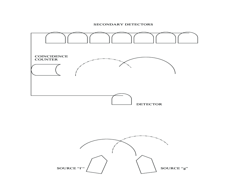
Figure 1: Arrangement for the detection of the particles. The set of secondary detectors covers all the directions where the detection probability is not negligible. The main detector and the secondary ones are connected to a coincidence counter to distinguish between events at the main detector triggered by one of two particles. The continuous and discontinuous circumference arcs represent, respectively, the particles ”f” and ”g”.

The second quantization formalism is a powerful technique for the description of multiparticle systems. In this framework, the particles are mathematically represented by the Schröndiger field operator. If we restrict to the stationary problem it is given by

$$\hat{\psi}({\bf r})=\int d^{3}{\bf q}\psi_{\bf q}({\bf r})\hat{a}({\bf q})$$ (1)

where the $\psi_{\bf q}({\bf r})$ form a complete basis of stationary wavefunctions labelled by the continuum index ${\bf q}$. On the other hand, $\hat{a}({\bf q})$ is the annihilation operator of the state ${\bf q}$. A common choice for the basis is that of plane waves parametrized by the momentum ${\bf p}$:

$$\hat{\psi}({\bf r})=\frac{1}{(2\pi\hbar)^{3/2}}\int d^{3}{\bf p}\exp{\left(\frac{i{\bf p}.{\bf r}}{\hbar}\right)}\hat{a}({\bf p})$$ (2)

The initial state in Fock’s space after the emission of the particles is (both particles are emitted by independent sources):

$$|I>=\int d^{3}{\bf p}\int d^{3}{\bf q}\;f({\bf q})g({\bf p})\hat{a}^{+}({\bf q})\hat{a}^{+}({\bf p})|0>$$ (3)

In this expression $|0>$ is the vacuum state and $f$ and $g$ are two functions of ${\bf q}$ and ${\bf p}$. When $f({\bf q})\neq\delta({\bf q}-{\bf q_{o}})$ and $g({\bf p})\neq\delta({\bf p}-{\bf p_{o}})$ with ${\bf q_{o}}$ and ${\bf p_{o}}$ arbitrary we deal with multimode states.

The parameters ${\bf p}$ and ${\bf q}$ refer to the same index used to parametrize the Schröndiger field operator. Every value of the parameters represents a different mode. With this choice every mode is a component of the same basis of wavefunctions used to write down the field operator As we only consider the stationary problem the modes refer to stationary wave functions, i. e., solutions of the one-particle stationary Schrödinger’s equation.

In order to simplify the presentation we assume that, $f$ and $g$ are real and non- negative functions. In this way they can be identified as the squared roots of the mode distributions, i. e., $f^{2}({\bf q})$ ($g^{2}({\bf p})$) gives the weight of the mode ${\bf q}$ (${\bf p}$) in the superposition of modes of the particle. The more general case of $f({\bf q})$ being a complex function (representing now $|f({\bf q})|^{2}$ the weight in the distribution) can be handled in a similar way, but the mathematical presentation would be more lengthy.

Note that in the above expression we have not explicitly included spin indexes. This is equivalent to assume that both particles in the same spin state. We use this simplification in order to clarify the analysis.

The probability of detection of only one particle at point ${\bf r}$ can be evaluated in the usual way [12]

$$P({\bf r})=\frac{<I|\hat{\psi}^{+}({\bf r})\hat{\psi}({\bf r})|I>}{<I|I>}$$ (4)

In this paper we shall refer to this probability as the detection probability. It gives the probability of detecting at point ${\bf r}$ one particle in a single repetition of the experiment. It is not to be confused with the detection efficiency, usually used in quantum optics or matter waves interferometry. The detection probability is closely related to the measured intensity, which is proportional to the number of detections in a large number of repetitions of the experiment. From the experimental point of view the detection probability is obtained from the measured intensity.

A better understanding of the physical meaning of the above formula can be obtained by comparison with similar expressions in quantum optics. An expression proportional to $<\hat{E}^{-}\hat{E}^{+}>$, with $\hat{E}=\hat{E}^{+}+\hat{E}^{-}$ the electric field operator, gives the rate of detection of photons by a phototube [13]. In particular, for single-mode beams the expectation value, $<\hat{E}^{-}\hat{E}^{+}>$, is proportional to the mean number of photons in the light beam. Consequently, the detection rate is proportional to the mean number of photons. Physically, this proportionality can be understood because ”the phototube measures the intensity of a light beam by counting the rate at which atomic ionizations take place, which is in turn proportional…..to the beam intensity” [13]. When multimode beams are considered $<\hat{E}^{-}\hat{E}^{+}>$ is no longer proportional to the mean number of photons, but can be interpreted as the observable beam intensity [13]. The detection rate is proportional to this observable intensity. In the case of massive particles the discussion follows similar lines. For particles in single-mode states the numerator of the r. h. s. of equation (4) is proportional to the mean number of particles in the state $|I>$. Therefore, assuming a connexion between the probability of detection and the mean number of particles similar to that discussed by Loudon between the detection rate and the mean number of photons we arrive at the usual interpretation of equation (4), which is extended to multimode states.

The calculation of the detection probability can be easily carried out using the (anti)commutation relations:

$$[\hat{a}({\bf p}),\hat{a}^{+}({\bf q})]_{\mp}=\delta^{3}({\bf p}-{\bf q})$$ (5)

In all the expressions with a double sign the upper and lower ones will refer, respectively, to bosons and fermions.

Note that in the last equation the spin indexes have not been included. This is a consequence of the previous assumption that both particles are in the same spin state. Then the general relation $[\hat{a}({\bf p},s),\hat{a}^{+}({\bf q},s^{\prime})]_{\mp}=\delta^{3}({\bf p}-{\bf q})\delta_{ss^{\prime}}$ transforms into the above equation.

First, we evaluate the denominator of Eq. (4) (as usual, the vacuum is normalized to unity $<0|0>=1$):

$$<I|I>=\int d^{3}{\bf p}\int d^{3}{\bf q}(f({\bf q})f({\bf p})g({\bf q})g({\bf p})\pm f^{2}({\bf q})g^{2}({\bf p}))$$ (6)

We assume the functions $f$ and $g$ to be normalized to unity

$$\int f^{2}({\bf p})d^{3}{\bf p}=1=\int g^{2}({\bf p})d^{3}{\bf p}$$ (7)

This is the usual normalization for one-particle states, where the spatial normalization $\int|\psi({\bf r})|^{2}d^{3}{\bf r}=1$, with $\psi({\bf r})=\int f({\bf p})\psi_{{\bf p}}({\bf r})d^{3}{\bf p}$ gives, via the orthonormality conditions, $\int\psi_{{\bf p}}^{*}({\bf r})\psi_{{\bf q}}({\bf r})d^{3}{\bf r}=\delta^{3}({\bf p}-{\bf q})$, equation (7).

With this choice equation (6) becomes

$$<I|I>=\pm 1+\int d^{3}{\bf p}\int d^{3}{\bf q}f({\bf q})f({\bf p})g({\bf q})g({\bf p})$$ (8)

This scalar product cannot be factored into the product of two one-particle scalar products. Moreover, when $f=g$ we have $<I|I>=0$ for fermions. This corresponds to the physically forbidden situation of two identical fermions. It is simple to show that the scalar product is zero or negative for fermions (property 1 in appendix A). The situation is similar to that found in the quantization of the free electromagnetic field [14]. However, the physically measurable magnitudes are the detection probabilities, which as we shall see later, are positive definite and, consequently, property 1 does not represent a problem at all (this scalar product would be positive by introducing $|I>\rightarrow i|I>$ for fermions, but then the notation for bosons and fermions would be different).

Evaluating the numerator of equation (4) results in the detection probability expression

$$P({\bf r})=\alpha_{fg}P_{fg}({\bf r})+\alpha_{fg}P_{fg}^{*}({\bf r})\pm\alpha_{gg}P_{ff}({\bf r})\pm$$

$$\alpha_{ff}P_{gg}({\bf r})=2\alpha_{fg}ReP_{fg}({\bf r})\pm\alpha_{gg}P_{ff}({\bf r})\pm\alpha_{ff}P_{gg}({\bf r})$$ (9)

where $Re(.)$ refers to the real part of the complex expression $(.)$,

$$\alpha_{fg}=\frac{\beta_{fg}}{<I|I>}$$ (10)

with

$$\beta_{fg}=\int d^{3}{\bf q}f({\bf q})g({\bf q})\;;\;\beta_{ff}=\beta_{gg}=1$$ (11)

and

$$P_{fg}({\bf r})=\int d^{3}{\bf q}\int d^{3}{\bf p}f({\bf q})g({\bf p})\psi_{{\bf q}}^{*}({\bf r})\psi_{{\bf p}}({\bf r})$$ (12)

The form of equation (9) is clearly that of an interference phenomenon. $P_{ff}$ and $P_{gg}$ are the detection probabilities one obtains when only particles of one of the two sources are emitted and detected. These probabilities are weighted by the coefficients $\alpha_{gg}$ and $\alpha_{ff}$. On the other hand, $2\alpha_{gf}ReP_{gf}$ is the interference term. It contains the contributions of the product of the wavefunctions of the two particles.

We note that the terms $P_{ff}$ and $P_{gg}$ would also be produced by a mixture of one-particle states, but the interference term clearly shows that we are dealing with a two-particle pure state.

When the particles have no common modes ($f\cap g=\o$) the interference term vanishes, property that agrees with the well- known origin of this type of interferences: the detector is unable to distinguish if a mode common to both particles has its origin in one or other of the sources. In quantum mechanics two indistinguishable alternatives give rise to interference patterns.

Note that in the case of fermions with equal mode distributions ($f=g$) the expression for the probability is undefined because both, the numerator and denominator of equation (4), are null. Physically this corresponds to the impossibility of measuring any property of a system of two identical fermions, since the two particles cannot be prepared in that two-particle state. We discuss this point to more extent in the example presented below and in appendix B.

We also remark that the detection probability is non-negative for fermions in spite of the fact that the denominator of equation (4) is negative or zero. This property that follows directly from the definition of the detection probability, can easily be checked from equation (9) which can be rewritten for fermions as $|\alpha_{ff}|P_{gg}+|\alpha_{gg}|P_{ff}+2\alpha_{gf}ReP_{gf}$. Then using equations (27) and (28) of the appendix (presented there for other purpose) we can easily see that this expression is non-negative.

We end this section presenting an example where all these expressions can be evaluated analytically. We assume both distribution functions to be Gaussians with equal spread:

$$f({\bf p})=N\exp{(-({\bf p}-{\bf f_{o}})^{2}/Q^{2})};g({\bf p})=N\exp{(-({\bf p}-{\bf g_{o}})^{2}/Q^{2})}$$ (13)

with $N=(2/\pi Q^{2})^{3/4}$ and $Q$ being constant factors, and ${\bf f_{o}}$ and ${\bf g_{o}}$ two constant vectors.

Using repeatedly the well-known formula $\int_{\infty}^{\infty}exp(\mu x^{2}+\eta x)dx=(\pi/-\mu)^{1/2}exp(-\eta^{2}/4\mu)$ for $Re(\mu)\leq 0$ we easily obtain:

$$<I|I>=\pm 1+exp({-({\bf f_{o}}-{\bf g_{o}})^{2}/Q^{2}})$$ (14)

$$\beta_{fg}=\exp{(-({\bf f_{o}}-{\bf g_{o}})^{2}/2Q^{2})}$$ (15)

and, finally, using as basis of the wave functions plane waves (see equation (2))

$$P({\bf r})=\frac{Q^{3}}{\sqrt{8}\hbar^{3}}\exp{(-Q^{2}{\bf r}^{2}/2\hbar^{2})}\times$$

$$\left(\frac{\pm 1+\exp{(-({\bf f_{o}}-{\bf g_{o}})^{2}/2Q^{2})}cos(({\bf f_{o}}-{\bf g_{o}}).{\bf r})/\hbar)}{\pm 1+\exp{(-({\bf f_{o}}-{\bf g_{o}})^{2}/Q^{2})}}\right)$$ (16)

We can easily check with this explicit model two characteristics found previously, the scalar product is negative or zero for fermions and the detection probability for fermions tends to an undefined expression of the type $0/0$ when ${\bf f_{o}}\rightarrow{\bf g_{o}}$. We show in appendix B that this indetermination cannot be removed by the application of L’Hôpital’s rule

Equation (16) shows clearly the existence of interference effects. The interference term is that with the cosine function. For an experiment with detectors placed at different positions we would have an oscillatory dependence on the position variable. However, we are only considering an experiment with the position of the detector fixed. Now, we can observe an oscillatory dependence in the detections at the fixed point if we vary ${\bf f_{o}}-{\bf g_{o}}$, i. e., for different compositions of the multimode states.

Note that this example can be described as a single mode situation if we consider a Gaussian modes basis (every particle is then in a single mode state). However, the results are similar for other multimode states that cannot be reduced to single mode states in particular modes basis.

Let us consider in the next sections the possibility of extending the concepts of distinguishability and visibility and their complementarity relations to this type of interference phenomena.

3 Distinguishability

Let us briefly review the definition of distinguishability in standard interferometry, for instance in the usual beam splitter experiment. The particle is prepared in a two-dimensional Hilbert space: $c_{1}|1>+c_{2}|2>$, representing $|1>$ and $|2>$ the two alternatives in the beam splitter, the two available pathways. Varying $c_{1}$ and $c_{2}$ we obtain different intensities at the detector placed at a fixed position, corresponding to an interference phenomenon. The distinguishability of the two alternatives is $||c_{1}|^{2}-|c_{2}|^{2}|$ [2].

In our arrangement we are concerned with modes instead of paths. The distinguishability must now refer to the differences between the mode distributions of both particles. Moreover, we distinguish between two particles instead of the usual approach, which considers alternatives of a one-particle system. A definition of distinguishability suitable for our experiment must meet three conditions:

1) If there are no common modes the distinguishability must reach its maximum value: both particles are completely distinguishable.

2) When the two particles are prepared in the same state (equal distribution of modes) the distinguishability must be minimal: both particles are identical an indistinguishable.

3) Following the usual convention the values of the distinguishability must be in the interval $[0,1]$.

We propose the following definition of distinguishability, which fulfills the three above criteria ($\beta_{fg}$ positive and $\beta_{fg}\leq 1$ (equation (27)) in the appendix A):

$$D=1-\frac{2\int f({\bf p})g({\bf p})d^{3}{\bf p}}{\int f^{2}({\bf p})d^{3}{\bf p}+\int g^{2}({\bf p})d^{3}{\bf p}}=1-\beta_{fg}$$ (17)

In the example of the Gaussian distribution this expression becomes

$$D=1-\exp{(-({\bf f_{o}}-{\bf g_{o}})^{2}/2Q^{2})}$$ (18)

that has value $0$ for $f=g$. For this type of distributions we do not have the case of no common modes because these distributions are never strictly zero. However, in the limit $2Q^{2}/({\bf f_{o}}-{\bf g_{o}})^{2}\rightarrow 0$, in which the number of common modes tends to zero, we have asymptotically $D\rightarrow 1$.

4 Contrast

In standard interferometry the measure of the visibility of the interference patterns is given by $(I_{max}-I_{min})/(I_{max}+I_{min})$, with $I_{max}$ and $I_{min}$ being the maximum and minimum values of the intensity (or probability of detection events). In the case of interference by a beam splitter the variation of the intensity is due to changes of values of $c_{1}$ and $c_{2}$ (see the first paragraph in the previous section). In diffraction granting experiments different intensity is obtained at each point after the granting.

In our case, by analogy, the visibility would be given by $V_{p}=(P_{max}-P_{min})/(P_{max}+P_{min})$, with $P_{max}$ and $P_{min}$ being the maximum and minimum values of the detection probability. However, this is not a satisfactory definition for our problem The aim of the paper would be a complementarity relation between $V_{p}$ and $D$. The distinguishability, as deduced in the previous section, is a function of $f$ and $g$: for every pair of distributions $f$ and $g$ we obtain a value of $D$. Therefore, an appropriate definition of visibility should assign a value of visibility to every pair of distributions. This is not the case for $V_{p}$: once $f$ and $g$ are given, as the position of the detector is fixed, the detection probability has a unique value. There are no maximum or minimum values of the detection probability, but a single value. We could compare the different values of the detection probability obtained varying $f$ and $g$ to determine $P_{max}$ and $P_{min}$. This way, however, we cannot assign a value of $V_{p}$ to every pair, $f$ and $g$, of distributions.

Other measure of visibility valid for continuous variables has been presented in the quantum optics literature, [9]. When broad band beams are considered their states are characterized by their distribution of power between phase and amplitude fluctuations. In the case of two-photon systems this power distribution refers to the intensity fluctuation correlations. These measurements are done via a homodyne detection system instead of photons counters. As in our arrangement we focus on the detection by ”particle counters” the way of measuring in [9] shows that it is not a measure of visibility appropriate for our problem.

We shall introduce the new measure, showing in this section that it is physically acceptable. Later, in the next section, we shall see that the new measure gives complementarity relations in some cases, justifying its introduction at posteriori.

In order to see how to do it we shall consider another interference experiment, the usual two-slit experiment with only one particle and with a fixed position for the detector. The source emits one particle in every repetition of the experiment, which travels to a screen with two slits. A detector is placed at a fixed position after the screen. If $\phi_{A}$ and $\phi_{B}$ denote the wavefunctions of the particle passing respectively through slit A or B (both normalized), the complete wavefunction of the particle is $(\phi_{A}+\phi_{B})/\sqrt{2}$, and the detection probability at the fixed position ${\bf r}$ of the detector becomes $\tilde{P}({\bf r})=\frac{1}{2}|\phi_{A}({\bf r})|^{2}+\frac{1}{2}|\phi_{B}({\bf r})|^{2}+Re(\phi_{A}^{*}({\bf r})\phi_{B}({\bf r}))$. As all the parameters of the problem are constant (the position of the detector and the wavefunction of the particle are fixed for all the repetitions of the experiment) the usual concept of visibility cannot be applied because we do not have variation of the probability detection and there are no maximum and minimum values. We have two contributions to the detection probability $\tilde{P}_{o}({\bf r})=\frac{1}{2}|\phi_{A}({\bf r})|^{2}+\frac{1}{2}|\phi_{B}({\bf r})|^{2}$ and $\tilde{P}_{I}({\bf r})=Re(\phi_{A}^{*}({\bf r})\phi_{B}({\bf r}))$. The first one corresponds to the detection probability in the absence of interference effects, i. e., the detection probability obtained when in every repetition of the experiment we close one of the slits avoiding one of the two alternatives for the particle and, consequently, also the interference effects. The interference effects are associated with $\tilde{P}_{I}$. A natural measure of the interference effects is given by comparing the probability detections in the presence and absence of the interference effects, i. e., by $\tilde{P}({\bf r})/\tilde{P}_{o}({\bf r})$ (valid for points where $\tilde{P}_{o}({\bf r})$ is not null). When there are no interference effects the ratio is 1. When the ratio is different from 1 we have interference effects whose strength is measured by the separation of the ratio with respect to 1. Other possible measure would be of the form $|\tilde{P}_{I}({\bf r})|/\tilde{P}_{o}({\bf r})$ (the absolute value of $\tilde{P}_{I}$ must be used in order to maintain the non-negative character of the measure). However, this definition does not distinguish between contributions of the interference effects that increase or decrease the detection probability. Consequently we disregard it.

Now we return to our original problem. Following the same arguments considered in the two-slit problem, the measure of the importance of the interference contribution to the probability detection must be based on the ratio between both types of probability detections. We propose the following definition which we shall name as contrast

$$C=\frac{P}{P_{o}}=1+\frac{2\alpha_{fg}Re(P_{fg})}{|\alpha_{gg}|P_{ff}+|\alpha_{ff}|P_{gg}}=1\pm\frac{2\beta_{fg}Re(P_{fg})}{P_{ff}+P_{gg}}$$ (19)

where $P$ is given by equation (9) and $P_{o}=|\alpha_{gg}|P_{ff}+|\alpha_{ff}|P_{gg}$. Note the absolute values for the $\alpha$ in the last expression; in this way we assure the positive definite character of $P_{o}$ and $C$ for fermions. We have also used the property $\alpha_{fg}=\pm|\alpha_{fg}|$ in the last step.

We analyse now some of the properties of the new definition. First, it is positive or zero as follows directly from the definition. It is defined at all the points where $P_{o}\neq 0$. We do not care about the singular points $P_{o}=0$. The values of the contrast are within the interval $[0,2]$. It is very simple to demonstrate the last statement taking into account that $\tilde{C}$ (defined by $C=1\pm\tilde{C}$) obeys the relation $|\tilde{C}|\leq 1$ (see property 2 of Appendix A). When $2\beta_{fg}Re(P_{fg})=0$ there are no interference effects and $C=1$. This condition is obtained in particular when there are no common modes for the two particles. This behaviour is similar for bosons and fermions. However, for other situations the behaviour is completely different. Let us consider the case $f=g$ (for fermions $f\rightarrow g$ because the limit $f=g$ is forbidden). For bosons $f=g$ leads to $C=2$. The detection probability doubles that without interference effects. On the other hand, for fermions with $f\rightarrow g$, $C\rightarrow 0$ reflecting the property that, contrarily to bosons, the detection probability tends to vanish. Because $Re(P_{fg})$ can be positive or negative we can have values $C>1$ or $C<1$ for both, bosons and fermions.

At first sight $|\tilde{C}|=|C-1|$ would also be a good definition of ”visibility”. However, there are two properties of $|\tilde{C}|$ that invalidate it as an acceptable candidate to replace the visibility. The first one is that it cannot distinguish between contributions of the interference term that enhance or diminish the detection probability. The argument follows closely that presented for $|\tilde{P}_{I}({\bf r})|/\tilde{P}_{o}({\bf r})$ in the case of the one-particle two-slit experiment. Depending on the fact of $Re(P_{fg})$ being positive or negative, the contributions to the detection probability have opposite sign. However, when we use $|\tilde{C}|$ we lost the information about the sign of the contribution of the interference term. We do not know if it tends to increase or to decrease the detection probability. Now, we consider the second property. One would expect that for large detection probabilities, i. e., for large increments of the detection probability due to the contribution of the interference term, the value of the variable measuring the contrast would increase. This is so for bosons, $|\tilde{C}|\rightarrow 1$ when $f\rightarrow g$ and the detection probability reaches its maximum value. However, for fermions when $f\rightarrow g$, $|\tilde{C}|$ tends to $1$, the maximum value of $|\tilde{C}|$; in spite of the fact that the detection probability tends to zero, its minimum value.

Finally, let us briefly discuss how to evaluate the contrast ratio. $P({\bf r})$ is directly obtained from the experimental detections values. $P_{o}({\bf r})$ can be evaluated combining the experimental determination of $P_{ff}$ and $P_{gg}$, and the knowledge (obtained in the preparation) of $\alpha_{ff}$ and $\alpha_{gg}$. The method is to carry out two different experiments with one-particle states. In the first one only one of the sources emits particles in the state $|f>=\int d^{3}{\bf q}f({\bf q})\hat{a}^{+}({\bf q})|0>$. The probability detection is $P_{ff}$. In the same way, in the second experiment using particles in the state $|g>$ we obtain experimentally $P_{gg}$. Now, with $\alpha_{ff}$ and $\alpha_{gg}$, which can be calculated from the preparation of the state, we obtain $P_{o}({\bf r})$, and we can evaluate the contrast. Equivalently, the contrast could be determined using $Re(P_{fg})$, which can be obtained from equation (9) using a method similar to that described above.

Based on the above considerations we conclude that contrast is a good measure of the quality of the interference effects considered in this paper. This is so because of three main reasons: (i)It gives a quantitative estimation of the contribution of the interference effects to the detection probability. (ii) As we shall see later, it allows for complementariry relations with distinguishability. (iii) It can be easily evaluated from the experimental data of detection and the knowledge of the initial state ($f$ and $g$ distributions). Contrast is a good measure for our arrangement, and also for the two-slit experiment discussed at the beginning of this section, i. e. , for experiments where the detection is restricted to a fixed position. If it is a good measure for other type of interference experiments should be analysed in every arrangement.

5 Complementarity relations

In standard interferometry there are complementarity relations between the distinguishability of the different paths available to the particle and the visibility of the interference patterns. We now look for the existence of complementarity relations between the distinguishability of the two particles and the contrast of the probability detection in our arrangement.

To analyse this problem we shall rest on the following inequality:

$$\frac{2\beta_{fg}Re(P_{fg})}{P_{gg}+P_{ff}}\leq\beta_{fg}$$ (20)

This inequality is equivalent to $2Re(P_{fg})/(P_{gg}+P_{ff})\leq 1$ (equation (28) in the appendix A). Note that we can assume $Re(P_{fg})\geq 0$ because if $Re(P_{fg})<0$, equation (20) automatically holds.

We analyse first the case of bosons. We have $C\leq 1+\beta_{fg}$, and

$$D+C\leq 2$$ (21)

This is a typical complementarity relation. When the distinguishability increases the contrast diminishes; a large distinguishability corresponds to a small number of common modes and small interference effects $P$ being close to $P_{o}$. In the limit of $D=1$ we have $C=1$. On the other hand, when $D$ is small we have a large number of common modes and large interference effects. In particular, in the limit $D=0$ we have $C=2$, the maximum value of the contrast.

The equality sign in the above expression is valid when equation (20) is an equality: $2Re(P_{fg})=P_{ff}+P_{gg}$, relation valid for $f=g$, i. e., when both particles have the same distribution and for some particular values of the $P$ when $f\neq g$.

We note that visibility and distinguishability enter in the standard complementarity inequality in a quadratic way, instead of the linear one found in the previous inequality. However, this is not a fundamental difference because our variables can be redefined as $D_{*}=D^{1/2}$ and $C_{*}=C^{1/2}$, becoming the above inequality $D_{*}^{2}+C_{*}^{2}\leq 2$.

We consider now the case of fermions. We obtain

$$D+C\geq 2(1-\beta_{fg})$$ (22)

Now, we do not have a complementarity relation. Physically, the non existence of a complementarity relation can be easily understood. Both, distinguishability and contrast show the same behavior (increase or decrease simultaneously) when their compositions ($f$ and $g$) vary, in contrast with the opposite behavior of bosons. For instance, when the number of common modes increases both, $C$ and $D$, diminish, the second one because unlike the case of bosons the interference contribution tends to cancel that of $P_{o}$.

We note that using $|\tilde{C}|$ as measure of the contrast one has complementarity relations for both, bosons and fermions. However, as discussed in the previous section, $|\tilde{C}|$ is not an acceptable measure of the contrast.

We conclude that there is a complementarity relation in the case of bosons. In contrast, such relation does not exist for bosons.

6 Conclusions

We have analysed in this paper the interference effects associated with the existence of common modes in the detection of one of the members of a multimode two-particle system. For simplicity we have restricted our considerations to real and non- negative functions $f$ and $g$, and states with equal spin for both particles. This particular case illustrates the most fundamental properties of the problem. The extension to the general problem where complex distributions $f$ and $g$ and other states with different spin values for the particles (which allow for other symmetric-antisymmetric combinations of the spin and spatial degrees of freedom of the particles) follows along similar lines but would be much more lengthy and will be considered in future work. The arrangement discussed in this paper is in the same line with the experiments considered in [7, 8, 10, 11]. The main novelties of our arrangement rest on the facts that the interference effects can be observed studying only the detection properties of one of the two particles and that it is directed to massive particles. It is important to note the relation with the Hanbury Brown-Twiss (HBT) experiment [15], and related intensity correlation arrangements. In our case we compare the events at the detector and the secondary detectors only in order to avoid double detection events in the main detector, not as in HBT to measure their correlations. Moreover, the comparison is not carried out as in HBT at two points, but at a point (where the main detector is placed) and at a large number of points (where the secondary detector are placed covering all the possible directions for the particles). The interference effects are not associated with the indistinguishability of the two particles, but with the existence of common modes (even in the case that both particles are not identical because their spectral composition is not equal). The experimental realization of this type of arrangement would be an interesting further step in two-particle interferometry with independent sources.

We have studied the possibility of extending the usual notions of distinguishability and visibility to our arrangement. The definition of distinguishability here proposed is different from the usual one in standard interferometry in two main aspects. First, it refers to the distinguishability of the two particles of the system instead of the usual distinguishability of a one- particle system. Second, it is based on the existence of common modes, not in the possibility of following different alternatives or available paths the particle.

We have also shown that the usual notion of visibility is not suitable for our problem. We have replaced it by the concept of contrast, based on the comparison of the detection probabilities with and without interference effects. The analytical form of the contrast as a function of $\beta_{fg}$ is different for bosons and fermions. We have also explored the existence of complementarity relations between distinguishability and contrast. They are obtained in the case of bosons (provided that the distribution functions obey equation (7)). These complementarity relations are an example of complementarity for the distinguishability in two-particle systems. Note that in the case of two-particle systems a complementarity relation has been demonstrated [2]. However the complementary variables are one- and two-particle visibilities, not distinguishability. In contrast, there is no complementarity relation for fermions. This is a new manifestation of the different behaviour of both types of particles. Of course, this result does not mean the impossibility of finding other measures of ”visibility” suitable for two-fermion systems in arrangements as the one here proposed or in other experiments previously carried out [16]. These measures would give rise to complementarity relations with the distinguishability. This possibility is an open problem that should be addressed in future work.

Finally, we shall consider the feasibility of experimentally carrying out the ideal arrangement presented in the paper. We focus on two points, the preparation of the beams and the data acquisition time. Photon beams can be prepared in multimode states (see, for instance, [7]). In the case of massive particles, trapping techniques can be used to prepare matter waves in multimode states. For instance, a thermal atomic cloud confined in a trap of width $L$ is described by a state superposition of the eigenfunctions of the trap. When the trap is opened adequately, the resulting beam can propagate in the desired direction. Each eigenfunction can be approximated by a wave packet with mean momentum proportional to $(n+1)/L$ ($n=0,1,..$), and momentum spread proportional to $1/L$ [17]. Using this type of techniques it seems possible, in principle, to prepare beams in multimode states with specific distributions as those described in this paper. On the other hand, we have the problem of reaching permissible data acquisition times. These limits have been considered by several authors (see, for instance, [18]), showing that for standard time windows of the coincidence counter the data acquisition time is within permissible limits. An important simplification of the detection scheme would be achieved if it would be experimentally demonstrated that the rate of double detections is negligible when compared to that of single events. Then we could eliminate the secondary detectors and the coincidence counter, shortening in a notorious way the data acquisition time. Once you have prepared the two particles in multimode and equal spin states, the experiment reduces to a simple detection and counting arrangement. In similar arrangements, but with only one source emitting in each repetition of the experiment, we can determine $P_{ff}$ and $P_{gg}$. Collecting all these data we can evaluate the contrast. On the other hand, the distinguishability is deduced from the preparation of the particles. Comparing both values we can test the relation between distinguishability and contrast. We conclude that making available sources of multimode states, the arrangement considered in previous sections could be experimentally realized.

Acknowledgments

This work has been partially supported by the DGICyT of the Spanish Ministry of Education and Science under Contract No. REN2000-1621 CLI. I am grateful to Joan Alcaide for helping in the preparation of the manuscript.

Appendix A: Two mathematical properties

In this Appendix we demonstrate the two following properties:

PROPERTY 1. For fermions $<I|I>\leq 0$.

We present a general demonstration of this property independent of the normalization of equation (7). For fermions we have equation (6) with the negative sign. We introduce the notation $N_{f}=\int d^{3}{\bf q}f^{2}({\bf q})$, $N_{g}=\int d^{3}{\bf q}g^{2}({\bf q})$, $F({\bf q})=f({\bf q})/\sqrt{N_{f}}$ and $G({\bf q})=g({\bf q})/\sqrt{N_{g}}$.

Using the inequality $(F({\bf q})-G({\bf q}))^{2}\geq 0$ we have

$$F({\bf q})G({\bf q})\leq\frac{1}{2}F^{2}({\bf q})+\frac{1}{2}G^{2}({\bf q})$$ (23)

Using these expressions we obtain

$$\int F({\bf q})G({\bf q})d^{3}{\bf q}\leq 1$$ (24)

and, finally

$$\int d^{3}{\bf q}\int d^{3}{\bf p}f({\bf q})g({\bf q})f({\bf p})g({\bf p})\leq N_{f}N_{g}$$ (25)

which is equivalent to

$$<I|I>\leq 0$$ (26)

PROPERTY 2. $|\tilde{C}|\leq 1$.

First, using as in property 1 that $(f({\bf q})-g({\bf q}))^{2}\geq 0$ we obtain (taking into account equation (7))

$$\beta_{fg}\leq 1$$ (27)

On the other hand, we have

$$|2Re(P_{fg})|\leq P_{ff}+P_{gg}$$ (28)

The last expression can be easily verified using the complex functions

$$\phi_{+}=\int d^{3}{\bf q}f({\bf q})\psi_{{\bf q}}+\int d^{3}{\bf q}g({\bf q})\psi_{{\bf q}}$$ (29)

and

$$\phi_{-}=\int d^{3}{\bf q}f({\bf q})\psi_{{\bf q}}-\int d^{3}{\bf q}g({\bf q})\psi_{{\bf q}}$$ (30)

Then as $\phi_{+}\phi_{+}^{*}=P_{ff}+P_{gg}+2Re(P_{fg})\geq 0$ and $\phi_{-}\phi_{-}^{*}=P_{ff}+P_{gg}-2Re(P_{fg})\geq 0$ we obtain equation (28) noting that $P_{ff}\geq 0$ and $P_{gg}\geq 0$.

Finally using equations (27) and (28) we obtain for $\tilde{C}=2\beta_{fg}Re(P_{fg})/(P_{ff}+P_{gg})$

$$|\tilde{C}|\leq 1$$ (31)

Appendix B: Application of L’Hôpital’s rule

It is usual to resort to L’Hôpital’s rule to elucidate the correct limit of expressions whose numerator and denominator tend simultaneously to $0$. This is the case of equation (16) for fermions when ${\bf f_{o}}\rightarrow{\bf g_{o}}$. With the notation $W_{1}$, $W_{2}$ and $W_{3}$ for the three components of the vector ${\bf f_{o}}-{\bf g_{o}}$, equation (16) can be expressed as $P({\bf W})\sim F({\bf W})=P_{N}({\bf W})/P_{D}({\bf W})$ with $P_{N}({\bf W})=-1+exp(-{\bf W}^{2}/2Q^{2})cos({\bf W}.{\bf r}/\hbar)$ and $P_{D}({\bf W})=-1+exp(-{\bf W}^{2}/Q^{2})$. In order that the limit exists when ${\bf W}\rightarrow{\bf 0}$ it must exist for any succession of ${\bf W}$ that tends to ${\bf 0}$. Let us consider, for instance, the succession $W_{1}^{*}\rightarrow 0$, $W_{2}^{*}=0$ and $W_{3}^{*}=0$. This way we reduce the problem to an one-dimensional one and we can use L’Hôpital’s rule in the standard way. As $lim_{W_{1}^{*}\rightarrow 0}P_{N}({\bf W^{*}})=lim_{W_{1}^{*}\rightarrow 0}P_{D}({\bf W^{*}})=0$, L’Hôpital’s rule states that if $lim_{W_{1}^{*}\rightarrow 0}(P_{N}^{\prime}({\bf W^{*}})/P_{D}^{\prime}({\bf W^{*}}))$ exists, it is the limit of $F({\bf W^{*}})$ for ${\bf W^{*}}\rightarrow{\bf 0}$. The evaluation is simple

$$P_{N}^{\prime}({\bf W^{*}})=\left(\frac{dP_{N}({\bf W^{*}})}{dW_{1}^{*}}\right)=-\frac{W_{1}^{*}}{Q^{2}}exp(-(W_{1}^{*})^{2}/2Q^{2})\times$$ (32)

$$cos(W_{1}^{*}x_{1}/\hbar)-\frac{x_{1}}{\hbar}exp(-(W_{1}^{*})^{2}/2Q^{2})sin(W_{1}^{*}x_{1}/\hbar)$$

and

$$P_{D}^{\prime}({\bf W^{*}})=\frac{-2W_{1}^{*}}{Q^{2}}exp(-(W_{1}^{*})^{2}/Q^{2})$$ (33)

In the limit $W_{1}^{*}\rightarrow 0$ both expressions tend to zero and we obtain again an indeterminate expression for their ratio. We apply again L’Hôpital’s rule and, with an obvious notation we obtain

$$P_{N}^{\prime\prime}({\bf W^{*}})=exp(-(W_{1}^{*})^{2}/2Q^{2})cos(W_{1}^{*}x_{1}/\hbar)\left(-\frac{1}{Q^{2}}-\frac{x_{1}^{2}}{\hbar^{2}}+\frac{(W_{1}^{*})^{2}}{Q^{4}}\right)$$

$$+\frac{2W_{1}^{*}x_{1}}{\hbar Q^{2}}exp(-(W_{1}^{*})^{2}/2Q^{2})sin(W_{1}^{*}x_{1}/\hbar)$$ (34)

$$P_{D}^{\prime\prime}({\bf W^{*}})=\frac{-2}{Q^{2}}\left(1-\frac{2(W_{1}^{*})^{2}}{Q^{2}}\right)exp(-(W_{1}^{*})^{2}/Q^{2})$$ (35)

The limit of $F({\bf W^{*}})$ when $W_{1}^{*}\rightarrow 0$ is

$$lim_{W_{1}^{*}\rightarrow 0}F({\bf W^{*}})=\frac{1}{2}\left(1+\frac{x_{1}^{2}Q^{2}}{\hbar^{2}}\right)$$ (36)

Now we can consider a different succession $\tilde{W}_{1}=\tilde{W}_{3}=0$ and $\tilde{W}_{2}\rightarrow 0$, reducing the problem again to a one-dimensional one, now in the axis ”2”. Following the same steps the limit is now

$$lim_{\tilde{W}_{2}\rightarrow 0}F({\bf\tilde{W}})=\frac{1}{2}\left(1+\frac{x_{2}^{2}Q^{2}}{\hbar^{2}}\right)$$ (37)

Clearly the limits for both successions are different (and so on for any other direction). Consequently, the limit when ${\bf W}\rightarrow{\bf 0}$ is not defined in a unique way: we have a different limit for every direction. $P({\bf W})$ remains undefined at ${\bf W}={\bf 0}$. Physically, this indetermination in the limit ${\bf W}\rightarrow{\bf 0}$ reflects the impossibility of obtaining definite quantum predictions for two-fermion systems in equal states, a two-particle state forbidden in quantum theory.

References

- [1] Greenberger D M and YaSin A 1988 Phys. Lett. A 128 391
- [2] Jaeger G, Shimony A and Vaidman L 1995 Phys. Rev. A 51 54
- [3] Englert B G 1996 Phys. Rev. Lett. 77 2154
- [4] Björk G and Karlsson A 1998 Phys. Rev. A 58 3477
- [5] Dürr S, Nonn T. and Rempe G 1998 Nature 395 33
- [6] Sancho P 2002 Physica Scripta 66 16
- [7] Walborn S P, de Oliveira A N, Padua S and Monken C H, quant-ph/0212017.
- [8] Hong C K, Ou Z Y and Mandel L 1987 Phys. Rev. Lett. 59 2044
- [9] Ralph T C 2000 J. Opt. B: Quantum Semiclass. Opt. 2 L31; 2000 Phys. Rev. A 61 044301
- [10] Pfleegor R L and Mandel L 1967 Phys. Rev. 159 1084
- [11] de Riedmatten H, Marcikic I, Tittel W, Zbinden H and Gisin N 2003 Phys. Rev. A 67 022301
- [12] Galindo A and Pascual P 1990 Quantum Mechanics (Springer-Verlag)
- [13] Loudon R 1973 The Quantum Theory of Light (Clarendon Press)
- [14] Itzykson C and Zuber J B 1987 Quantum Field Theory (McGraw-Hill)
- [15] Hanbury Brown R and Twiss R Q 1956 Nature 177 27
- [16] Kiesel H, Renz A and Hasselbach F 2002 Nature 418 392
- [17] Andersson E, Calarco T, Folman R, Hessmo B and Schmiedmayer J quant-ph/0107124v3.
- [18] Kodama T, Osakabe N, Endo J, Tonomura A, Ohbayashi K, Urakami T, Ohsuka S, Tsuchiya H, Tsuchiya Y and Uchikawa Y 1998 Phys. Rev. A 57 2781