Slow transport by continuous time quantum walks

Abstract

Continuous time quantum walks (CTQW) do not necessarily perform better than their classical counterparts, the continuous time random walks (CTRW). For one special graph, where a recent analysis showed that in a particular direction of propagation the penetration of the graph is faster by CTQWs than by CTRWs, we demonstrate that in another direction of propagation the opposite is true; In this case a CTQW initially localized at one site displays a slow transport. We furthermore show that when the CTQW’s initial condition is a totally symmetric superposition of states of equivalent sites, the transport gets to be much more rapid.

The transfer of information over discrete structures (networks) which are not necessarily regular lattices has become a topic of much interest in recent years. The problem is relevant to many distinct fields, such as polymer physics, solid state physics, biological physics and quantum computation, see Refs. Bouchaud and Georges (1990); Albert and Barabási (2002); Dorogovtsev and Mendes (2002); Kempe (2003); van Kampen (1990); Weiss (1994) for reviews. In particular, quantum mechanics seems to allow a much faster transport than classically possible. Thus, recent studies of quantum walks on graphs show that these often outperform their classical counterparts, i.e., in terms of the penetrability of the graph, for an overview see Ref. Kempe (2003) and references therein. We recall that the extension of classical random walks to the quantum domain is not unique. There exist different variants of quantum walks, such as discrete Aharonov et al. (1993) and continuous time Farhi and Gutmann (1998) versions, which are not equivalent to each other. Here we focus on walks in continuous time.

Walks occur over graphs which are collections of connected nodes. To each graph corresponds a discrete Laplace operator (sometimes also called adjacency or connectivity matrix), ${\bf A}=(A_{ij})$. Here the non-diagonal elements $A_{ij}$ equal $-1$ if nodes $i$ and $j$ are connected by a bond and $0$ otherwise. The diagonal elements $A_{ii}$ equal the number of bonds which exit from node $i$, i.e., $A_{ii}$ equals the functionality $f_{i}$ of the node $i$.

Classically, assuming the transmission rates of all bonds to be equal, say $\gamma$, the continuous-time random walk (CTRW) is governed by the master equation Weiss (1994)

$$\frac{\rm d}{{\rm d}t}p_{j}(t)=\sum_{k}T_{jk}\ p_{k}(t),$$ (1)

where $p_{j}(t)$ is the probability to find at time $t$ the walker at node $j$. ${\bf T}=(T_{jk})$ is the transfer matrix of the walk, which is related to the adjacency matrix by ${\bf T}=-\gamma{\bf A}$. Equation (1) is spatially discrete, but it also admits extensions to continuous spaces, e.g., leading to the disordered Lorentz gas model, which describes the dynamics of an electron through a disordered substrate Mülken and van Beijeren (2004).

We stick with the spatially discrete situation and let now the CTRW start from node $k$, i.e., we set $p_{k}(0)=\delta_{jk}$. Denoting by $p_{jk}(t)$ the conditional probability of being at node $j$ at time $t$ when starting at node $k$ at $t=0$ leads to

$$\frac{\rm d}{{\rm d}t}p_{jk}(t)=\sum_{l}T_{jl}\ p_{lk}(t),$$ (2)

which is another way to write Eq.(1) van Kampen (1990); Weiss (1994). Given the linearity of these equations, their solution involves a simple integration. For Eq.(2) we have formally

$$p_{jk}(t)=\langle j|e^{{\bf T}t}|k\rangle.$$ (3)

Figure 1: (a) Graph consisting of two Cayley trees of generation $G=3$. (b) horizontal projection of the graph following Ref. Childs et al. (2002), (c) vertical projection of the same graph. (d) Vertical projection of a similar graph, obtained from two Cayley trees of general generation $G$, indicating the new nodes (clusters) and the $d_{k}$, see text for details.

We now turn to one quantum mechanical extension of the problem, the so-called continuous-time quantum walk (CTQW). CTQWs are obtained by assuming the Hamiltonian of the system to be ${\bf H}=-{\bf T}$ Farhi and Gutmann (1998); Childs et al. (2002). Then the basis vectors $|k\rangle$ associated with the nodes $k$ of the graph span the whole accessible Hilbert space. In this basis the Schrödinger equation reads

$$i\frac{\rm d}{{\rm d}t}|k\rangle={\bf H}|k\rangle,$$ (4)

where we set $\hbar\equiv 1$. The transition amplitude $\alpha_{jk}(t)$ from state $|k\rangle$ at time $0$ to state $|j\rangle$ at time $t$ is then

$$\alpha_{jk}(t)=\langle j|e^{-i{\bf H}t}|k\rangle.$$ (5)

According to Eq.(4) the $\alpha_{jk}(t)$ obey

$$i\frac{\rm d}{{\rm d}t}\alpha_{jk}(t)=\sum_{l}H_{jl}\alpha_{lk}(t).$$ (6)

The inherent difference between Eq.(3) and Eq.(5) is, apart for the imaginary unit, the fact that classically $\sum_{j}p_{jk}(t)=1$, whereas quantum mechanically $\sum_{j}|\alpha_{jk}(t)|^{2}=1$ holds.

We turn now to the graph displayed in Fig. 1(a). The graph is obtained from two finite Cayley trees of generation $G$ which have a common set of end nodes along the horizontal symmetry axis indicated in Fig. 1(a), Farhi and Gutmann (1998); Childs et al. (2002). For the nodes on the axis as well as for the top and bottom nodes the connectivity is $f=2$, whereas for all other nodes $f=3$.

The authors of Refs. Farhi and Gutmann (1998) and Childs et al. (2002) have analyzed CTQWs over the graph given in Fig. 1(a), focussing on walks which start at the top node, and looking for the amplitude, Eq.(5), of being at the bottom node at time $t$. The problem can then be simplified by considering only states which are totally symmetric superpositions of states $|k\rangle$ involving all the nodes $k$ in each row of Fig. 1(a), as indicated schematically in Fig. 1(b). The transport gets then mapped onto a one-dimensional CTQW Childs et al. (2002).

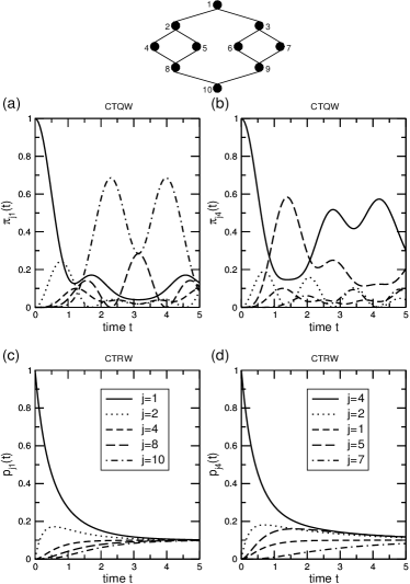
Figure 2: Top: Graph obtained from two Cayley-trees of generation $G=2$. Below: Probabilities for the CTQW, (a) and (b), and for the CTRW, (c) and (d), to be at node $j$ after time $t$ when starting at time $0$ from node 1 or from node 4. Left column, (a) and (c): Starting node is the top node 1. Right column, (b) and (d): Starting node is the leftmost node 4. The time is given in units of the inverse transmission rate $\gamma^{-1}$, see text following Eq.(1).

Given that CTQWs obey time inversion, so that they never reach a limiting distribution, one uses the quantity Aharonov et al. (2001)

$$\chi_{jk}=\lim_{T\to\infty}\frac{1}{T}\int_{0}^{T}dt\ |\alpha_{jk}(t)|^{2}.$$ (7)

to compare the efficiency of CTQWs to that of CTRWs. We will show in the following that the $\chi_{jk}$ may depend strongly on the initial state. Now, as shown in Childs et al. (2002), based on Eq.(7), the CTQW’s probability of being at the bottom node when starting at the top node is considerably larger than that of CTRWs.

One legitimate question to ask now is: What happens if one considers on the same graph CTQWs which start at the leftmost node and end at the rightmost node? As we proceed to show, it turns out that then the transport by CTQWs gets to be much slower than the transport by CTRWs. We start by focussing on the full solution of Eq.(6), for which all the eigenvalues and all the eigenvectors of ${\bf T}=-{\bf H}$ (or, equivalently, of ${\bf A}$) are needed. For, say, the 22 nodes of Fig. 1(a) we have to solve the eigenvalue problem for ${\bf A}$ (or ${\bf T}$), which is a real and symmetric $22\times 22$ matrix. This is a well-known problem, also of much interest in polymer physics Blumen et al. (2003, 2004), and many of the results obtained there can be used for our problem here.

We recall first that the matrix ${\bf A}$ is non-negative definite. Then, for a structure like the one in Fig. 1(a), ${\bf A}$ has exactly one vanishing eigenvalue, $\lambda_{0}=0$, the remaining eigenvalues being positive. Let $\lambda_{n}$ denote the $n$th eigenvalue of ${\bf A}$ and ${\bf\Lambda}$ the corresponding eigenvalue matrix. Furthermore, let ${\bf Q}$ denote the matrix constructed from the orthonormalized eigenvectors of ${\bf A}$, so that ${\bf A}={\bf Q}{\bf\Lambda}{\bf Q}^{-1}$. Now the classical probability is given by

$$p_{jk}(t)=\langle j|{\bf Q}e^{-t\gamma{\bf\Lambda}}{\bf Q}^{-1}|k\rangle.$$ (8)

For the quantum mechanical transition probability it follows that

$$\pi_{jk}(t)\equiv|\alpha_{jk}(t)|^{2}=|\langle j|{\bf Q}e^{-it\gamma{\bf\Lambda}}{\bf Q}^{-1}|k\rangle|^{2}.$$ (9)

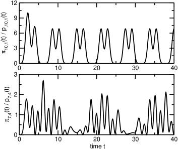
Figure 3: Ratios $\pi_{jk}(t)/p_{jk}(t)$ for different directions of propagation, (a) top-bottom walk and (b) left-right walk over time $t$, see Fig.2 for units and details.

In order to determine numerically the corresponding eigenvalues and eigenvectors of the matrix ${\bf A}$ for different graphs we have used the standard software package MAPLE 7. We start by considering the smaller graph, $G=2$, given at the top of Fig. 2. The figures show the transition probabilities for CTQWs and CTRWs starting at the top node 1 (left column), which corresponds to the situation described in Childs et al. (2002), or at the leftmost node 4 (right column). Remarkably, CTQWs starting at the top node reach the opposite node 10 very quickly, see Fig. 2(a), much quicker than expected from the CTRW behavior, Fig. 2(c). However, for walks starting at the leftmost node 4 and going to the rightmost node 7, the probabilities for the CTQWs, Fig. 2(b), and the CTRWs, Fig. 2(d), get to be comparable. Furthermore, the CTQWs’ probabilities, $\pi_{4,4}(t)$ and $\pi_{1,1}(t)$, of return to the starting node within the time interval depicted in Fig. 2 are much higher if the walks start at the leftmost node 4 of the graph instead of at the top node 1. On the other hand, for CTRWs there is not much difference between starting at the leftmost or at the top node, only that in the first case it just takes a little bit longer to reach an uniform distribution, compare Fig. 2(c) and Fig. 2(d).

We now extend the time interval to $t=40$ and compare the efficiency of the CTQW transport to the CTRW one. In Fig. 3 we plot for the top-bottom and the left-right walks the ratio of the quantum mechanical probabilities $\pi_{jk}(t)$ to the classical ones $p_{jk}(t)$. For top-bottom transport, depicted in Fig. 3(a), the plot turns out to be highly regular, reflecting the high symmetry of the underlying graph in the vertical direction. For left-right transport the plot is less regular. Note the different scaling of the ordinates in the two parts of Fig. 3, which again stresses the preferential role played by the transport in top-bottom direction.

In order to discuss what happens at even longer times, we proceed to evaluate for the CTQW the limiting distributions $\chi_{jk}$ given by Eq. (7). For CTRWs the limit is simple: All $p_{jk}(t)$ tend to the same constant, which is the inverse of the total number of nodes in the graph, no matter where the CTRWs start. For the CTQWs, however, this is not the case, as can already be inferred from Figs. 2 and 3. Hence, we compute $\chi_{jk}$ for the top-bottom and for the left-right cases separately. Therefore, for the $G=2$ graph we compute the eigenvalues and eigenvectors of the respective $10\times 10$ matrix ${\bf A}$ and the $\chi_{jk}$ by using MAPLE. Having the appropriate eigenvalue matrix ${\bf\Lambda}$ and the matrix ${\bf Q}$ constructed from the orthonormalized eigenvectors we find with Eqs. (7) and (9) and the LinearAlgebra package of MAPLE that for the top-bottom case

$$\chi_{10,1}=0.2644>\frac{1}{10},$$ (10)

whereas for the left-right case

$$\chi_{7,4}=0.0545<\frac{1}{10}.$$ (11)

Thus, the limiting CTRW-probability, $1/10$, lies between $\chi_{7,4}$ and $\chi_{10,1}$. The top-bottom CTQW is more, the left-right CTQW less efficient than the corresponding CTRW.

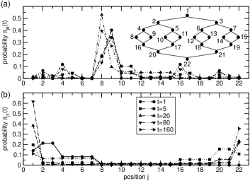
Figure 4: Transition probabilities $\pi_{jk}(t)$ for a CTQW on the $G=3$ graph starting at (a) the leftmost node, $\pi_{j8}(t)$, and (b) starting at the top node, $\pi_{j1}(t)$, for times $t=1$, $5$, $20$, $80$, and $160$, see Fig.2 for units and details.

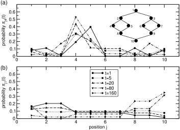
Figure 5: Transition probability for a CTQW on the $G=2$ graph starting at (a) the leftmost node, $\pi_{j4}(t)$, and (b) at the top node, $\pi_{j1}(t)$, for times $t=1$, $5$, $20$, $80$, and $160$, see Fig.2 for units and details.

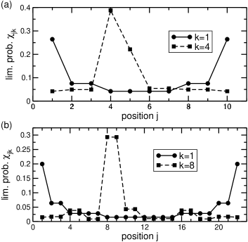
Figure 6: Limiting probability $\chi_{jk}$ for a CTQW on the (a) $G=2$ graph and on the (b) $G=3$ graph. Starting points are the top node, $k=1$ and the leftmost nodes $f=4$ and $k=8$, respectively.

In order to better visualize that the top-bottom and left-right $\chi_{jk}$ are very different, we show in Figs. 4 and 5 the quantum mechanical transition probabilities $\pi_{jk}(t)$ for all nodes $j$ when starting (a) at the leftmost node 8 and (b) at the top node 1; in these figures the time is displayed parametrically. Figure 4 is for the $G=3$ graph and Fig. 5 for the $G=2$ graph. Now, even for the small graphs considered here, we find differences in the transition probabilities, which clearly depend on the initial node. For the $G=3$ graph consisting of $22$ nodes, the CTQW starting at the top node 1 spreads out rapidly over the whole graph. After a very short time interval, there is a large probability to find the walker at the bottom node 22, see Fig. 4(b). However, for the CTQW starting at the leftmost node 8, we have up to times $t=160$ a high probability of finding it in the left half of the graph, see Fig. 4(a). Therefore, the propagation of the CTQW is strongly dependent on the starting node. For the smaller $G=2$ graph of Fig. 5, which consists of $10$ nodes, the effect is similar, but slightly less pronounced.

We illustrate the situation at very long times in Fig. 6, where we display the limiting probabilities $\chi_{jk}$ for the $G=2$ and the $G=3$ graphs, see Eq.(7). For a CTQW starting at the top node 1 the limiting probability distribution has its maximum at the end nodes of the graphs, i.e. at nodes 1 and 10 for $G=2$, and at nodes 1 and 22 for $G=3$. For a CTQW starting at the leftmost node, $k=4$ for $G=2$ and $k=8$ for $G=3$, the limiting probability distribution shows a strong maximum around the starting node.

Other initial conditions for the CTQW are, indeed, possible, especially when considering the high symmetry of the underlying graphs. Note that, using for instance the site enumeration of Fig. 4, a CTQW from node $8$ to node $15$ is equivalent to a CTQW from, say, node $10$ to node $14$. The graph’s symmetry suggests to collect groups of such nodes into clusters, while focussing on the transport from left to right. It is then natural to view the nodes 8, 9, 10, and 11 as belonging to the first cluster. The second cluster consists then of the nodes 4, 5, 16, and 17, all of which are directly connected by one bond to the nodes of the first cluster. The nodes 2 and 20 of the third cluster are all nodes directly connected by one bond to the nodes of the second cluster, while at the same time not belonging to the first cluster. In general, all the nodes of the $(k+1)$st cluster are connected by one bond to nodes of the $k$th cluster and at the same time do not belong to the $(k-1)$st cluster.

Let us denote the number of nodes in cluster $k$ by $d_{k}$. The transport occurs now from a cluster to the next, by which the original graph gets mapped onto a line in which one new node corresponds to a group of original nodes of the graph. For a new node at position $k\in[2,G]$ we find that $d_{k}=2^{G-k+1}$, the same being true for the mirror node value, i.e., $d_{k}=d_{2G+2-k}$. Note that for the end nodes $d_{1}=d_{2G+1}=2^{G-1}$, the same holds for the nodes next to them. Moreover, for the middle node $d_{G+1}=2$.

We now focus on the transport via the states which are totally symmetric, normalized, linear state-combinations for all the original nodes in each cluster. Thus, for the $k$th cluster, whose sites we denote by $n$, we have as a new state

$$|a_{k}\rangle=\frac{1}{\sqrt{d_{k}}}\sum_{n\in k}|n\rangle.$$ (12)

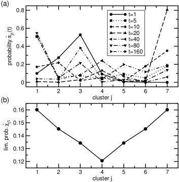
Figure 7: (a) Transition probability $\tilde{\pi}_{j1}(t)$ for a CTQW between different clusters $j$ of the $G=3$ graph. The CTQW starts at the first cluster, presented is the situation at times $t=1$, $5$, $10$, $20$, $40$, $80$, and $160$, see Fig.2 for units and details. (b) Limiting probability $\tilde{\chi}_{j1}$ for a CTQW starting at the first cluster.

The CTQW is now determined by the new Hamiltonian $\tilde{\bf H}=\gamma\tilde{\bf A}$, where the matrix elements of $\tilde{\bf A}$ are obtained from the new basis states $|a_{k}\rangle$ and from the matrix ${\bf A}$ through

$$\tilde{A}_{jk}=\langle a_{j}|{\bf A}|a_{k}\rangle.$$ (13)

Given the properties of ${\bf A}$ and the construction of the $|a_{k}\rangle$, Eq.(12), $\tilde{\bf A}$ is a real and symmetrical tridiagonal matrix, which implies a CTQW on a line. The diagonal elements of $\tilde{\bf A}$ are given by

$$\tilde{A}_{kk}=\langle a_{k}|{\bf A}|a_{k}\rangle=\frac{1}{d_{k}}\sum_{{n\in k}\atop{n^{\prime}\in k}}\langle n^{\prime}|{\bf A}|n\rangle=f_{n}\equiv f_{k},$$ (14)

where $f_{k}$ is the functionality of every node in the $k$th cluster. For the sub- and super-diagonal elements of $\tilde{\bf A}$ we find

$$\tilde{A}_{k,k+1} = \tilde{A}_{k+1,k}=\langle a_{k}|{\bf A}|a_{k+1}\rangle$$ (15)

$$= \frac{1}{\sqrt{d_{k}d_{k+1}}}\sum_{{n\in k}\atop{n^{\prime}\in k+1}}\langle n^{\prime}|{\bf A}|n\rangle=-\frac{b_{k}}{\sqrt{d_{k}d_{k+1}}},$$

where $b_{k}$ is the number of bonds between the clusters $k$ and $k+1$. Now, except for the ends and the center of the graph, $b_{k}$ equals the maximum of the pair $(d_{k},d_{k+1})$. Between the central node ($d_{G+1}=2$) and its neighbors ($d_{G}=d_{G+2}=2$) the number of bonds is $b_{G}=b_{G+2}=2$. The number of bonds between the end node and its neighbor is $b_{1}=b_{2G+1}=2d_{1}=2^{G}$.

For the graph consisting of 22 original nodes the new matrix $\tilde{\bf A}$ is a tridiagonal $7\times 7$ matrix, which can be readily diagonalized. The advantage of the procedure is clear: the new matrix $\tilde{\bf A}$ depends on the number of clusters and grows with ($2G+1$), whereas the full adjacency matrix, ${\bf A}$, grows with the total number of nodes in the graph, namely with ($3\cdot 2^{G}-2$).

From Eq.(12) the transition amplitude between the state $|a_{k}\rangle$ at time 0 and the state $|a_{j}\rangle$ at time $t$ is given by

$$\tilde{\alpha}_{jk}(t)=\langle a_{j}|e^{-i\tilde{\bf H}t}|a_{k}\rangle=\langle a_{j}|\tilde{\bf Q}e^{-i\gamma\tilde{\bf\Lambda}t}\tilde{\bf Q}^{-1}|a_{k}\rangle,$$ (16)

where $\tilde{\bf\Lambda}$ is the eigenvalue matrix and $\tilde{\bf Q}$ the matrix constructed from the orthonormalized eigenvectors of the new matrix $\tilde{\bf A}$.

Now the quantum mechanical transition probabilities are given by $\tilde{\pi}_{jk}(t)=|\tilde{\alpha}_{jk}(t)|^{2}$. Figure 7(a) shows the transition probabilities for CTQWs over clusters. Remarkably now, and similar to Fig. 4(b), already in rather short periods of time such CTQWs move from one end cluster to the other. The limiting probability distribution, $\tilde{\chi}_{jk}$, which is depicted in Fig. 7(b), also supports this finding. Note that Fig. 7(b) again reflects the symmetry of the original graph.

In conclusion, we have shown that CTQWs do not necessarily perform better than their CTRWs counterparts. By focussing on a particular graph, we have shown that the penetration of such a graph by CTQWs can be better or worse than the one by CTRWs, depending on the initial state and on the propagation direction under scrutiny.

Support from the Deutsche Forschungsgemeinschaft (DFG) and the Fonds der Chemischen Industrie is gratefully acknowledged.

References

- Bouchaud and Georges (1990) J.-P. Bouchaud and A. Georges, Phys. Rep. 195, 127 (1990).
- Albert and Barabási (2002) R. Albert and A.-L. Barabási, Rev. Mod. Phys. 74, 47 (2002).
- Dorogovtsev and Mendes (2002) S. N. Dorogovtsev and J. F. F. Mendes, Adv. Phys. 51, 1079 (2002).
- Kempe (2003) J. Kempe, Contemporary Physics 44, 307 (2003).
- van Kampen (1990) N. van Kampen, Stochastic processes in physics and chemistry (North-Holland, 1990).
- Weiss (1994) G. H. Weiss, Aspects and applications of the random walk (North-Holland, 1994).
- Aharonov et al. (1993) Y. Aharonov, L. Davidovich, and N. Zagury, Phys. Rev. A 48, 1687 (1993).
- Farhi and Gutmann (1998) E. Farhi and S. Gutmann, Phys. Rev. A 58, 915 (1998).
- Mülken and van Beijeren (2004) O. Mülken and H. van Beijeren, Phys. Rev. E 69, 046203 (2004).
- Childs et al. (2002) A. M. Childs, E. Farhi, and S. Gutmann, Quantum Information Processing 1, 35 (2002).
- Aharonov et al. (2001) D. Aharonov, A. Ambainis, J. Kempe, and U. Vazirani, in Proceedings of ACM Symposium on Theory of Computation (STOC’01) (2001), p. 50.
- Blumen et al. (2003) A. Blumen, A. Jurjiu, Th. Koslowski, and C. von Ferber, Phys. Rev. E 67, 061103 (2003).
- Blumen et al. (2004) A. Blumen, C. von Ferber, A. Jurjiu, and Th. Koslowski, Macromolecules 37, 638 (2004).