On the Temperature Dependence of the Casimir Effect

Abstract

The temperature dependence of the Casimir force between a real metallic plate and a metallic sphere is analyzed on the basis of optical data concerning the dispersion relation of metals such as gold and copper. Realistic permittivities imply, together with basic thermodynamic considerations, that the transverse electric zero mode does not contribute. This results in observable differences with the conventional prediction, which does not take this physical requirement into account. The results are shown to be consistent with the third law of thermodynamics, as well as being not inconsistent with current experiments. However, the predicted temperature dependence should be detectable in future experiments. The inadequacies of approaches based on ad hoc assumptions, such as the plasma dispersion relation and the use of surface impedance without transverse momentum dependence, are discussed.

I Introduction

There are many corrections that one in principle has to take into account when calculating the Casimir force between two bodies; the corrections may come from finite temperatures, finite extensions of the plates used in the experiments, corrugations on the plates, etc. (Recent reviews of the Casimir effect can be found in Refs. milton04 ; milton01 ; bordag01 .) The correction that we will be concerned with in the present paper is the one coming from finite temperatures. For the most part, we will consider the temperature dependent Casimir force between a compact sphere of radius $R$ and a plane substrate. The sphere is situated at a fixed distance $a$ from the plane ($a$ denotes the minimum distance between the surfaces). The sphere and the substrate are assumed nonmagnetic, but we consider the case where they may be made from different materials. We will moreover assume the proximity force theorem blocki77 to hold; this means that $a$ must be much less than $R$. (For corrections to this see Refs. jaffe04 ; Gies ; Emig .) On experimental grounds it is evidently desirable to calculate the Casimir forces in a realistic way. We will here take advantage of the excellent numerical dispersive data to which we have access for the materials gold and copper (and also aluminum) (courtesy of Astrid Lambrecht and Serge Reynaud). We know how the permittivity $\varepsilon(i\zeta)$ varies with imaginary frequency $\zeta$ over seven decades, $\zeta\in[10^{11},10^{18}]$ rad/s. We use these data to calculate the forces at two different temperatures, namely at room temperature, $T=300$ K, and at $T=1$ K. The latter temperature is conveniently attainable numerically, and it can for all practical purposes be identified with zero temperature. (The lowest temperature that we actually tested was $T=0.2$ K. If T becomes lower, we leave the frequency domain for our numerical dispersion data. It turns out that there are very small deviations between calculated values of the force for $T=1$ K and for $T=0.2$ K.) We obtain in this way a realistic picture of the finite temperature correction for these materials.

It ought to be emphasized that we are not adopting the so-called modified ideal metal (MIM) model, which assumes unit reflection coefficients for all but the transverse electric (TE) zero mode [see Eq. (11) below]; rather, we are using real data together with the assertion (based on thermodynamical and electrodynamical arguments) that the TE zero mode is absent, as that is an isolated point which cannot be extracted from data alone. Our approach is that which we have followed in other recent papers milton04 ; hoye03 ; brevik04 . The absence of a TE zero mode contribution to the Casimir effect for a real metal was discussed in detail in Ref. hoye03 , and also in Ref. sernelius04 . The result of this assumption, for instance, in the MIM model is the presence of a linear temperature term in the expression for the Casimir force between two planes, in the limit where $aT\ll 1$. The calculation for a real metal yields a linear temperature correction for low, but not too low temperatures, so that for very low temperatures the force and the free energy have zero slope. By contrast, in the conventional (old) model for an ideal metal (IM) the TE zero mode is included, and it implies that this linear temperature term is omitted. We ought to stress here that at $T=0$ the mentioned difference between a MIM and an IM model goes away, as the contributions from the zero frequency TE mode as well as from the zero frequency TM mode become buried in an integral over imaginary frequencies from zero to infinity.

The experiments of immediate interest for the present theory are the atomic force microscopy (AFM) tests, performed in particular by Mohideen et al. mohideen98 . A point that we ought to emphasize here is that previous analyses have most likely overestimated the accuracy of the AFM experiments. Thus the recent paper of Chen et al. chen04 , which is based upon a reanalysis of the experiment of Harris et al. (listed in mohideen98 ), claims an over-all experimental precision to be at the 1 percent level. In that apparatus a gold-coated polystyrene sphere mounted on a cantilever of an AFM was brought close to a metallic surface and the deflection was measured. However, as discussed in Refs. iannuzzi04 ; milton04 , at the very short distance of 62 nm (the minimum distance) the force at $a=62\,\mbox{nm}+\delta$ differs from the force at $a=62$ nm by more than 3.5 pN (the experimental uncertainty claimed by the authors) when $\delta$ is larger than a few angstroms. This means that $a$ should have been measured with atomic precision in order to correspond to the accuracy claimed. As for temperature corrections, these were found in chen04 to be negligible, this being related to their acceptance of the plasma dispersion relation for the material.

As the absence of the zero frequency TE mode has been controversial, we give in Sec. IV a discussion of this in view of recent work by Bezerra et al. bezerra04 They argue that this mode should be present. In Sec. V we give additional support to our arguments by showing that for a pair of anisotropic polarizable particles the Casimir force can vanish in certain directions as the temperature increases towards $\infty$, and although there are regions of negative entropy connected with the Casimir effect, there is no indication that thermodynamics is violated. Violation of thermodynamics is used as an argument by Bezerra et al. bezerra04 to require the presence of the TE zero mode. The inadequacy of using a surface impedance approach without including transverse momentum dependence is briefly reviewed in Sec. VI.

In this paper we put $\hbar=c=k_{B}=1$.

II General Formalism and Dispersive Properties

Let the sphere of radius $R$ be nonmagnetic, and have a permittivity $\varepsilon_{1}$. As mentioned, the sphere is situated a distance $a$ above a plane substrate; we let the nonmagnetic substrate have permittivity $\varepsilon_{2}$. According to the proximity force theorem blocki77 the attractive force $\cal{F}$ between sphere and plane at temperature $T$ can in the limit $a/R\ll 1$ be given approximatively as the circumference of the sphere times the surface free energy density $F$ in the parallel-plate configuration: ${\cal{F}}=2\pi RF(a)$. Following essentially the notation of Ref. hoye03 we can then write the force as

$${\cal{F}}=\frac{R}{\beta a^{2}}{\sum_{m=0}^{\infty}}^{\prime}\int_{m\gamma}^{\infty}y\,dy\left[\ln(1-\Delta_{1}^{\rm TM}\Delta_{2}^{\rm TM}e^{-2y})+\ln(1-\Delta_{1}^{\rm TE}\Delta_{2}^{\rm TE}e^{-2y})\right].$$ (1)

Here $y$ is the dimensionless quantity $y=qa$, and

$$q=\sqrt{k_{\perp}^{2}+\zeta_{m}^{2}},\quad\zeta_{m}=2\pi m/\beta,\quad\gamma=2\pi a/\beta,$$ (2)

${\bf k_{\perp}}$ being the component of $\bf k$ parallel to the plates in the parallel-plate configuration. Further, $\zeta_{m}$ with $\beta=1/T$ are the Matsubara frequencies, and $\gamma$ is the dimensionless temperature. Superscripts TM and TE in Eq. (1) refer to the transverse magnetic and electric modes. The prime on the sum means that the zero mode has to be counted with half weight. With the conventional Lifshitz variables defined as

$$s=\sqrt{\varepsilon-1+p^{2}},\quad p=q/\zeta_{m},$$ (3)

we define the two kinds of $\Delta$’s, the reflection coefficients for a single interface, as

$$\Delta^{\rm TM}=\frac{\varepsilon p-s}{\varepsilon p+s},\quad\Delta^{\rm TE}=\frac{s-p}{s+p}$$ (4)

for each medium 1 and 2, respectively. If the two media are equal, $\Delta_{1}=\Delta_{2}$ for each kind of mode, then

$$(\Delta^{\rm TM})^{2}\equiv A_{m},\quad(\Delta^{\rm TE})^{2}\equiv B_{m},$$ (5)

where $A_{m},\,B_{m}$ are the TM, TE coefficients defined in Ref. hoye03 . Note that $s_{1}=\sqrt{\varepsilon_{1}-1+p^{2}},\,s_{2}=\sqrt{\varepsilon_{2}-1+p^{2}}$, with $p=q/\zeta_{m}$ being the same quantity in the two cases. The permittivities $\varepsilon(i\zeta_{m})$ are functions of the imaginary Matsubara frequencies $\zeta_{m}$. In the general case where the media are dispersive, $\Delta^{\rm TM}$ and $\Delta^{\rm TE}$ depend both on $p$ and on the Matsubara integer $m$. If the media are nondispersive, $\Delta^{\rm TM}$ and $\Delta^{\rm TE}$ are functions of $p$ only, independent of $m$.

As a general warning, we mention that the proximity theorem assumed here requires $a/R$ to be very small. Thus, within the framework of the optical path method recently considered by Jaffe and Scardicchio jaffe04 , believed to be more robust than the proximity approximation, disagreement with the latter approximation was found already when $a/R$ became larger than a few percent, whereas the method they propose agrees accurately with the recent exact numerical result of Gies et al. Gies .

II.1 Dispersive properties

As mentioned in the Introduction, we will use accurate numerical data for the variation of $\varepsilon$ with frequency for two different substances: gold and copper. These data refer to room temperature measurements. For gold, the data are shown graphically in Refs. lambrecht00 ; hoye03 . For frequencies up to about $1.5\times 10^{15}$ rad/s (note that 1 eV=$1.519\times 10^{15}$ rad/s), the data are nicely reproduced by the Drude dispersion relation

$$\varepsilon(i\zeta)=1+\frac{\omega_{p}^{2}}{\zeta(\zeta+\nu)},$$ (6)

where for gold the plasma frequency is $\omega_{p}=9.0$ eV and the relaxation frequency $\nu=$ 35 meV. For $\zeta>2\times 10^{15}$ rad/s the Drude curve however lies below the experimental curve.

All the dispersive data, of which we are aware, refer to room temperature. Now, as we will be interested in the Casimir force also at low temperatures, we are faced with the problem of how to estimate the permittivity $\varepsilon(i\zeta,T)$ under such circumstances. Numerical trials indicate rather generally that the Casimir force is very robust under variations in the input values for the permittivity, but at least this issue is a matter of principle. One possible way to proceed is to write the permittivity as

$$\varepsilon(i\zeta,T)=1+\frac{\omega_{p}^{2}}{\zeta[\zeta+\nu(T)]},$$ (7)

and make use of the Bloch-Grüneisen formula for the temperature dependence of the electrical resistivity $\rho$. This problem was discussed in Appendix D of Ref. hoye03 . One may in this way estimate the temperature relaxation frequency to be, in eV,

$$\nu(T)=0.0847\left(\frac{T}{\Theta}\right)^{5}\int_{0}^{\Theta/T}\frac{x^{5}e^{x}dx}{(e^{x}-1)^{2}},$$ (8)

where $\Theta=175$ K for gold. This formula implies that $\varepsilon(i\zeta,T)$ is somewhat higher for low $T$ than for $T=300$ K (cf. Fig. 1 in hoye03 ), when the frequencies are less than about $10^{14}$ rad/s. It is instructive to compare with the parallel-plate configuration, where it is known that the most important frequencies for the Casimir force are lying in the region $\zeta a\sim 1$. For $a=1\,\mu$m it corresponds to $\zeta\approx 2.5\times 10^{14}$ rad/s. For smaller gap widths—where the metallic properties of the medium fade away and its plasma properties become more dominant—it follows that the most important frequencies become higher. Taking all things together, we expect that the influence from the temperature variation in $\nu(T)$ is rather small. Some numerical trials that we have done support this expectation.

Another important point to be mentioned here is that the Bloch-Grüneisen argument sketched above neglects the effect from impurities. These give rise to a nonzero resistivity at zero temperature khoshenevisan79 . This fact strengthens our argument for setting the contribution from the Casimir force from the TE zero mode for a metal equal to zero. The issue has been considered in detail also by Sernelius and Boström sernelius04 ; bostrom00 . As one can see from Fig. 2 in sernelius04 , there exists a temperature dependent contribution to the Casimir force from the TE modes. This temperature dependence occurs for low frequencies at low temperature and extends to higher frequencies with increasing temperature. However, the temperature influence fades away before the the first nonzero Matsubara frequency is reached. It is therefore permissible to neglect the temperature dependence in $\nu(T)$. What remains important in $\nu$ is the constant term $\nu(T=0)\neq 0$ that is due to elastic scattering. The consequence is that

$$\zeta^{2}[\varepsilon(i\zeta)-1]\to 0,\quad\mbox{as}\quad\zeta\to 0,$$ (9)

so from (4) $\Delta^{\rm TE}$ vanishes at $m=0$. If one neglects this crucial constant $\nu(T=0)$, one can end up with a violation of the Nernst heat theorem bezerra02 . See also Boström and Sernelius bostrom04 for related discussion of these points.

Therefore, in the following we will restrict ourselves to using the room-temperature values for $\nu$ throughout, even when calculating ${\cal{F}}(T)$ at different temperatures. Even with this simplification, we point out that the temperature dependence in the Casimir force turns up in a rather complex way. Namely, the temperature occurs at three different places:

(i) in the prefactor in Eq. (1);

(ii) in the lower limit of the integral;

(iii) in the dependence of $\Delta^{\rm TM,TE}_{1}$ and $\Delta_{2}^{\rm TM,TE}$ on $T$ via the Matsubara frequencies in the permittivity: $\varepsilon=\varepsilon(i2\pi mT)$.

III Numerical Results

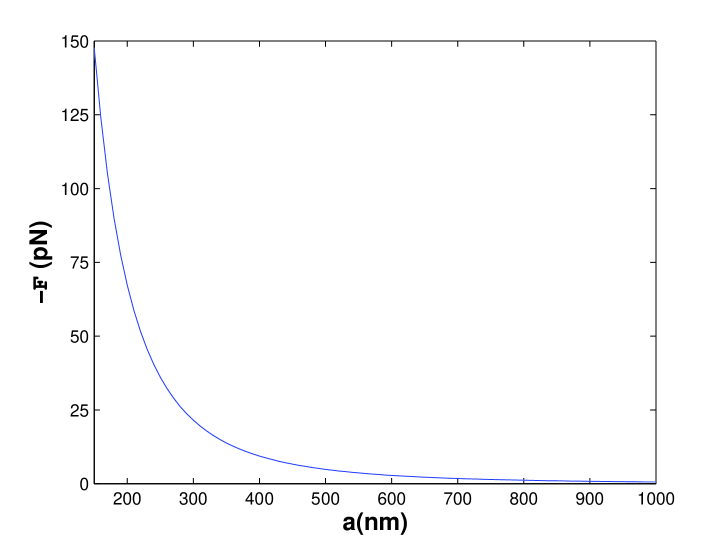
Figure 1: Force ${\cal F}$ between a gold sphere and a gold plate versus gap $a$, when $T=300$ K and $R=296$ $\mu$m.

Figure 1 shows, for a gold sphere and a gold plate, how the attractive force ${\cal F}(a)$ varies with $a$ in the interval from about 150 nm to 1 $\mu$m, when $R=296$ $\mu$m and $T=300$ K. As mentioned, the empirical data for $\varepsilon(i\zeta)$ are directly usable as input in Eq. (1). When $a=200$ nm, the force is calculated to be 67.22 pN.

A similar calculation can be made for a very low temperature, in order to show the magnitude of the temperature influence in the force. We assume throughout, as mentioned earlier, that $\nu=35$ meV. Using MATLAB we found $T=1$ K to be a numerically stable and reasonable lower limit. This temperature is moreover low enough to be identifiable with $T=0$ for all practical purposes.

We ought to stress that we choose to perform the $T\approx 0$ calculation numerically, inserting realistic data for $\varepsilon(i\zeta)$. This is in principle different from the conventional $T=0$ calculation for an idealized metal, where one simply puts $\varepsilon=\infty$ for all frequencies. (Recall that at $T=0$ the difference between a MIM and an IM model goes away, because of the very close spacing between the Matsubara frequencies.)

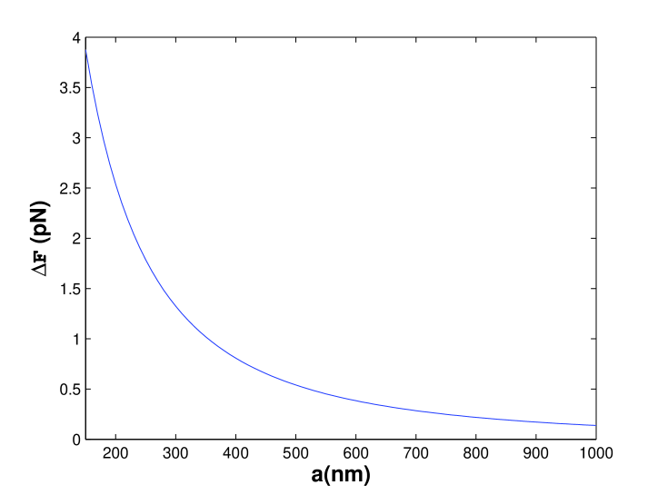
Figure 2: Force difference $\Delta{\cal F}=|{\cal F}\,(1\,\rm{K})|-|{\cal F}\,(300\,{\rm K})|$ between a gold sphere and a gold plate, versus gap $a$ for $R=296$ $\mu$m.

Rather than showing the calculated result for ${\cal F}(1\,{\rm K})$ explicitly, we show in Fig. 2 the difference between the forces, $\Delta{\cal F}$, defined as

$$\Delta{\cal F}={\cal F}\,(300\,{\rm K})-{\cal F}\,(1\,\rm{K})=|{\cal F}\,(1\,\rm{K})|-|{\cal F}\,(300\,{\rm K})|.$$ (10)

An important property seen from this curve is that $\Delta{\cal F}$ is positive. The force is thus weaker at room temperature than at $T=0$. This is the same effect as was found in Fig. 5 in hoye03 . This behavior is thus a consequence of Lifshitz’ formula plus realistic input data for the permittivity; there are no further assumptions involved. When $a=200$ nm, we find $\Delta{\cal F}$= 2.54 pN, which means that the force is reduced by 3.6 percent compared to the $T=0$ case.

For larger distances, $a=400$ nm, the temperature effect becomes larger. Thus for $a=400$ nm the force is 9.38 pN at $T=300$ K and 10.19 pN at $T=1$ K, yielding a 7.9 percent reduction at room temperature. At $a=1\;\mu$m, the corresponding numbers are 0.59 pN at $T=300$ K and 0.73 pN at $T=1$ K, which means a 19 percent reduction. This agrees in magnitude well with the temperature corrections in the case of parallel-plate geometry, as is seen from Fig. 5 in Ref. hoye03 .

Admitting an error of $10^{-8}$ in the $m$ summation in Eq. (1), we found the necessary number of terms to be in excess of 34000 in the case of the lowest separation investigated numerically, $a=50$ nm (not shown in the figure). When $a=200$ nm, about 11000 terms were required. At larger separations the necessary number of terms became considerably reduced; thus the case $a=1\,\mu$m corresponded to about 2700 terms.

The calculation of the force between a gold sphere and a copper plate gave very similar results. Thus for $a=200$ nm the force was 67.19 pN at $T=300$ K and 69.75 pN at $T=1$ K, corresponding to a reduction of 3.7 percent at room temperature. At $a=1\,\mu$m, the forces turned out to be the same (to the accuracy of two decimals) as in the Au-Au case.

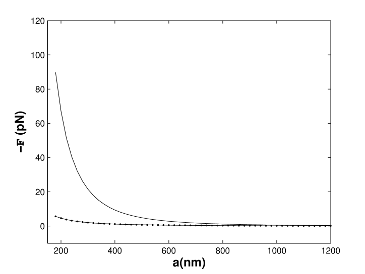
Figure 3: Force ${\cal F}$ between a gold sphere and a copper plate versus $a$, when $T=300$ K and $R=296$ $\mu$m. Bottom curve is the $m=0$ contribution.

In Fig. 3 we show, by the full line, how the force between a gold sphere and a copper plate varies with $a$, at $T=300$ K. The curve is calculated from Eq. (1), using the empirical data for these two materials directly. Our reason for giving this curve anew, in spite of its identity with the curve in Fig. 1 for all practical purposes, is that we have supplied the following new element, namely at the bottom of the figure we show explicitly the contribution from the $m=0$ term to the force. Namely, for the MIM model in which $A_{0}=1,\,B_{0}=0,\,A_{m}=B_{m}=1$ for $m\geq 1$ hoye03 , we have for the free energy

$$\beta F^{\rm MIM}=\frac{1}{4\pi}\int_{0}^{\infty}q\,dq\ln(1-e^{-2qa})+\frac{1}{\pi}\sum_{m=1}^{\infty}\int_{\zeta_{m}}^{\infty}q\,dq\ln(1-e^{-2qa}),$$ (11)

showing the $m=0$ contribution in the first term. Thus

$$\beta F^{\rm MIM}(m=0)=-\frac{\zeta(3)}{16\pi a^{2}},$$ (12)

meaning that the corresponding force contribution $2\pi RF^{\rm MIM}(m=0)$ becomes

$${\cal F}^{\rm MIM}(m=0)=-\frac{\zeta(3)}{8}\frac{R}{\beta a^{2}}.$$ (13)

From the figure this term contributes an increasing part of the total force for increasing $a$, and gives the full contribution in the classical limit $a\rightarrow\infty$.

We would like to make a direct comparison of our prediction with the recent experiment of Decca et al. decca03 ; decca03a . This experiment measured the Casimir force between a gold sphere and a copper plate by means of a microelectromechanical torsional oscillator, for separations in the range 0.2–2 $\mu$m. The radius of the sphere was $296\pm 2$ $\mu$m, thus the same radius as we have assumed above. Their measured values are shown, for instance, in Fig. 3 in Ref. decca03 . However, the scale of their figure for the total force prevents comparison with our numerical results with sufficient accuracy to draw firm conclusions about the magnitude of the temperature dependence.

But Fig. 3 in Ref. decca03 also gives a comparison with theoretical values by plotting the difference. These theoretical values are evaluated at $T=0$, but as we do, they also use a Drude model to obtain the dielectric constant in the limit of low frequencies. Then they find a small temperature correction with the same sign as we have theoretically predicted.

From Fig. 3 in Ref. decca03 we estimate $\Delta\cal F$ to be around 1 pN for $a=200$ nm, and to be too small to be discernible for large gaps, $a\geq 600$ nm (the scatter of the experimental points is considerable). This can be compared with our Fig. 2, where we calculated $\Delta\cal F$ to be 2.56 pN for $a=200$ nm and 0.14 pN for $a=1\,\mu$m. This reasonably good agreement between experimental and theoretical results is encouraging, and it indicates that our finite temperature calculations are on the right track.

We should also mention that Ref. decca03a refers to dynamical measurements that are claimed to rule out our results. However, we believe that the systematic theoretical and experimental uncertainties in this measurement are larger than estimated by those authors. In particular, we re-emphasize the uncertainty of measuring the Casimir force due to uncertainties in estimating a systematic shift of position as earlier discussed by Iannuzzi et al. iannuzzi04 and Milton milton04 , as mentioned in the Introduction.

IV Comment upon the Transverse Electric Zero Mode

Bezerra et al. bezerra04 claim that the Drude dielectric function for metals cannot be used in the theory for the Casimir force. Their opinion is that it violates the Nernst theorem in thermodynamics and is furthermore ruled out by a recent experiment. Instead the plasma relation should be used for the dielectric function. The latter implies the presence of a transverse electric mode at zero frequency besides the static dipole-dipole interaction; the latter being the zero-frequency limit of the transverse magnetic mode. Including such an transverse electric mode adds a term linear in temperature to the Casimir force by which it is increased by a factor of two in the high temperature limit.

These authors point to the standard theory, sketched above in Sec. II.1 where the relaxation parameter $\nu$ varies with temperature $T$ and vanishes at $T=0$. This is then a situation where in principle a transverse electric zero mode might be present in the Casimir force although it should not be present according to Maxwell’s equations of electromagnetism. However, its presence for $\nu=0$, but not otherwise, would make physical phenomena discontinuous as then $\nu=0$ will give something different from taking the limit $\nu\rightarrow 0$. Also we question whether a possible vanishing of the relaxation parameter at $T=0$ can dictate the behavior for $T>0$ where $\nu>0$. (As a remark we here note that strictly speaking the statistical mechanical derivation is exact only for dielectric functions independent of temperature, i.e., when induced dipole moments are harmonic oscillators. A $T$-dependence reflects anharmonicity. But we do not expect that this is of crucial significance here.)

As a result, Bezerra et al. bezerra04 conclude that the Drude dielectric function is thermodynamically inconsistent and cannot be used to calculate the thermal Casimir force for metals. However, we on the contrary have shown that it is thermodynamically consistent leading to zero entropy at $T=0$ in accordance with the Nernst theorem hoye03 . Thus, for $T>0$ a negative entropy contribution due to electromagnetic interaction between media is allowed as long as the total entropy is positive. We have earlier studied a simplified model in this regard hoye03 . The model consists of three harmonic oscillators. Two of them are the analogues of the two media that interact via the electromagnetic field represented by the third oscillator.

In the beginning of their Sec. III, Bezerra et al. bezerra04 state that our derivations were based upon a constant relaxation parameter $\nu$. However, we did not require such a limitation, only that $\nu(0)$ is finite. And as the authors further note, the value of $\nu$ is commonly very small, but nevertheless finite, at $T=0$ due to impurities, and as a result the entropy becomes zero at $T=0$ as required. Then they write that the negative entropy we found at $T=5\times 10^{-4}$ K is a violation of the Nernst theorem. But such a negative perturbing entropy is not a violation of the Nernst theorem since $T$ is finite as already discussed above. The further discussion about relaxation time, impurities, and surface impedance does not invalidate the use of a finite $\nu(0)$.

These authors further remark that we consider nonzero wave vectors $\bf k_{\bot}$ for which the reflection coefficient $r^{2}_{\bot}(0,k_{\bot})=0$. But this does not mean that reflection properties are different for the fluctuation field compared to real photons as we deal with only one such quantity; and as discussed above, thermodynamics is not violated. (See Sec. VI below for further discussion of $\mathbf{k_{\perp}}$ dependence.)

They further note that a material with dielectric constant $\varepsilon=100$, like a metal, gives a Casimir force that decreases with temperature in some interval and thus implies a negative entropy contribution. They conclude that such a material cannot exist as it would violate thermodynamics. Then they claim that real media with such large $\varepsilon$ are commonly polar for which $\varepsilon$ rapidly reduces to its optical value connected to its electronic polarizability. So with plate (or plate-sphere) separation of $1\,\mu{\rm m}$ the Casimir force again becomes monotonically increasing with $T$. However, this does not preserve the monotonic character of the Casimir force in general because one can just increase the plate separation. Non-monotonic behavior will then reappear when this separation exceeds a wavelength corresponding to the relaxation frequency (where $\varepsilon$ decreases rapidly).

In Sec. IV of their paper, they again conclude that the use of the Drude dielectric function in the Lifshitz formula violates the third law of thermodynamics (the Nernst heat theorem). This conclusion, stated as a rigorous proof, is made on the basis that the relaxation parameter will be much less than the Matsubara frequencies. But this is not a rigorous proof as the relaxation parameter will violate this inequality sufficiently close to $T=0$ (assuming $\nu(0)>0$). Furthermore the Drude dielectric function does not predict a linear temperature correction to the Casimir force all the way down to zero temperature. As we have shown earlier the Casimir force flattens out and becomes independent of temperature at $T=0$ in accordance with thermodynamics hoye03 ; brevik04 . (But the sharpness of this flattening increases with decreasing $\nu$.)

We further remark that the use of the Drude dielectric function is consistent with the $\varepsilon\rightarrow\infty$ limit (for large separation of the plates). Use of the plasma model ($\nu=0$), however, will give a discontinuous jump of the force in this limit. Such a jump is not expected for a continuous change in a physical parameter. Also for real metals the $\varepsilon$ effectively will be finite due to the finite size of the plane-sphere configuration. (Here one can note that a medium consisting of separate metal spheres of finite size will be like a polarizable medium with finite polarizability and dielectric constant.)

Finally the authors in Ref. bezerra04 conclude that use of the Drude dielectric function (6) is in contradiction with experiment. However, so far as we can see, experiments performed at a single temperature are at present too uncertain to draw conclusions about temperature variations. This seems even more evident from Ref. chen04 . There detailed analysis of experimental uncertainties are performed and various corrections for very short separations are estimated. They find an uncertainty of 1.75 % at 95 % confidence level for 62 nm separation. This uncertainty increases to 37.3 % for 200 nm. Earlier it has been remarked by others iannuzzi04 that such experiments are very sensitive to accurate determinations of plate separation since the plate-sphere Casimir force is proportional to the inverse cube of separation distance. However, the authors assert that they avoid this problem by making a least squares fit of the resulting data by which zero separation is pinpointed with an uncertainty of 0.15 nm. But in view of the uncertainties of the experiment this does not seem to resolve the disputed temperature dependence as heavy weight is put on the shortest separation of 62 nm where the force is by far the largest and changes most rapidly. Thus high apparent precision can be obtained for this separation (1.75 %) while for larger separations the uncertainties are rapidly increasing until they become larger than the magnitude of the disputed thermal effect. According to the authors of Ref. chen04 the thermal effect in dispute is about 1-2 % for 62 nm.

Very recently, a paper has appeared valeri giving the microscopic theory of the Casimir effect. These authors convincingly demonstrate that the TE zero mode cannot contribute, although the plasma model gives such a contribution.

V Anisotropic Particles with Negative Casimir Entropy

As mentioned above the appearance of a negative Casimir entropy for metals in a region of nonzero temperatures has been disputed with the claim that it violates the Nernst theorem of thermodynamics bezerra04 . However, as we argue this negative entropy region does not imply violation of thermodynamics since the Casimir free energy is a perturbing one and is not the total free energy of two interacting systems. Many such examples are known in statistical mechanics, including that of three interacting oscillators discussed in Ref. hoye03 . To illustrate this point, we here will consider a pair of particles with strong anisotropic polarizability and thus polarizable only in the $z$-direction, e.g., they may be metal needles. The result for a pair of particles with isotropic polarizability is well known and was rederived in a novel way by Brevik and Høye brevik88 .

The latter derivation is easily generalized to anisotropic particles. Using the path integral formalism the dipole-dipole interaction of the radiation field is given by Eq. (I5.9). (Here and below the numeral I refers the the equations of the reference mentioned.) Equation (I5.9) gives the interaction energy

$$\beta\Phi(12)=\eta\sum\limits_{n=-\infty}^{\infty}[\psi_{D\zeta_{n}}(r)\,D_{\zeta_{n}}(12)+\psi_{\Delta\zeta_{n}}(r)\,\Delta_{\zeta_{n}}(12)]a_{1\zeta_{n}}a_{2\zeta_{n}}^{*}$$ (14)

with

$$D_{\zeta_{n}}(12)=3({\bf\hat{r}\cdot\hat{a}}_{1\zeta_{n}})({\bf\hat{r}\cdot\hat{a}}_{2\zeta_{n}}^{*})-{\bf\hat{a}}_{1\zeta_{n}}\cdot{\bf\hat{a}}_{2\zeta_{n}}^{*},$$ (15)

$$\Delta_{\zeta_{n}}(12)={\bf\hat{a}}_{1\zeta_{n}}\cdot{\bf\hat{a}}_{2\zeta_{n}}^{*}$$ (16)

where the Matsubara frequency $\zeta_{n}=2\pi n/\beta$. The dipole radiating fields $\psi$ are given in (I5.10). Hats denote unit vectors. The ${\bf\hat{a}}_{\zeta_{n}}$ are unit vectors of the Fourier-transformed fluctuating dipole moments along the “polymer” path and $\eta\rightarrow 0$ is the discretized step length along the “polymers” that represent quantized particles in the path integral formalism.

The Casimir free energy times $-2\beta$ is now obtained from the average of expression (14) squared in accordance with (I3.5). For the isotropic case one has the average $\eta\langle{\bf a}_{\zeta_{n}}{\bf a}_{\zeta_{n}}^{*}\rangle=3\alpha_{\zeta_{n}}$ where $\alpha_{\zeta_{n}}$ is the polarizability. This follows from Eq. (I5.3). For the strongly anisotropic situation to be considered below one likewise will find ($z$ denotes the $z$-component)

$$\eta\langle a_{z\zeta_{n}}a_{z\zeta_{n}}^{*}\rangle=\alpha_{z\zeta_{n}}$$ (17)

as the only nonzero average as polarizations in $x$- and $y$-directions are zero in the present case.

Furthermore let the positions of the particles relative to each other be such that the $z$-component of ${\bf\hat{r}}$ equals $1/\sqrt{3}$. With this the $D_{\zeta_{n}}(12)$ will vanish as polarizations are present only in the $z$-direction. (With this relative position the corresponding electric field is transverse to the $z$-direction and thus to each of the dipole moments, i.e., there is no interaction connected to the $D_{\zeta_{n}}(12)$-term.) Thus only the $\Delta_{\zeta_{n}}(12)$-term remains. So with polarizations restricted to the $z$-direction Eq. (I5.14) turns into

$$-\beta F=\frac{1}{2}\sum\limits_{n}\alpha_{z\zeta_{n}}^{2}\psi_{\Delta\zeta_{n}}^{2}(r)$$ (18)

or with (I5.10) inserted the free energy is

$$F=-\frac{1}{\beta r^{6}}\sum\limits_{n=-\infty}^{\infty}\left(\frac{2}{3}\tau^{2}\right)^{2}e^{-2\tau}\alpha_{z\zeta_{n}}^{2}$$ (19)

where

$$\tau=\frac{2\pi r}{\beta\hbar c}|n|$$ (20)

as given by (I5.12).

As usual Eq. (19) gives a negative free energy. However, in the classical limit $T\rightarrow\infty$ the Casimir free energy (19), and thus the corresponding force, both vanish since only the $n=0$ term will contribute. Furthermore with this free energy the contribution to the entropy must be negative (or at least mainly negative) as $S=-\partial F/\partial T$, because $F$ must have a generally positive slope, but $S=0$ at $T=0$ as it should.

VI Surface Impedance

Most recently, Mostepanenko et al. geyer03 ; bezerra04 , apparently conceding that their arguments favoring the plasma model over the Drude model for the dispersion relation for real metals could not be supported either thermodynamically, electrodynamically, or experimentally, have asserted that for real metals one should use in the reflection coefficients in the Lifshitz formula not the bulk dielectric permittivity but the surface impedance. Indeed there is much to be said for using the latter. However, in may be shown in general that there is in fact no difference between the reflection coefficients computed using either description brevik04 . There is a one-to-one correspondence between the permittivity $\varepsilon$ and the surface impedance $Z$, which is given by the ratio of the transverse electric and magnetic fields at the surface. This correspondence, however, necessitates in general that both quantities possess dependence on the transverse momentum $\bf k_{\perp}$. As optical data strongly suggest that this dependence is usually negligible in the permittivity, a strong dependence on $\bf k_{\perp}$ is required in $Z$ brevik04

$$Z^{\rm TE}(\zeta,k_{\perp})=-\frac{\zeta}{\sqrt{\zeta^{2}\varepsilon(i\zeta)+k_{\perp}^{2}}}.$$ (21)

The vanishing of $1+Zq/\zeta$ at $\zeta=0$ demonstrates again that the TE zero mode does not contribute to the Casimir force. (Note that this vanishing happens in the Drude, but not the plasma model.) In contrast, Ref. geyer03 ; bezerra04 completely disregard this transverse momentum dependence and moreover make an ad hoc extrapolation from the infrared region to zero frequency milton04 . The inadequacy of neglecting the transverse momentum dependence has been stressed by Esquivel and Svetovoy esquivel04 .

VII Conclusions

In this paper we have sharpened our arguments in favor of using real data for the dielectric functions to apply the Lifshitz formula to calculate the force between metal surfaces, in particular between a spherical lens and a flat plate. In principle, one can also use the surface impedance to calculate this force, and although optical data is lacking for the latter, such use should yield the same result. In contrast, the procedures advocated in Refs. chen04 ; bezerra04 ; bezerra02 ; decca03 ; decca03a ; geyer03 contain ad hoc elements and assumptions.

We show both by direct computation, and through analogous models, that there is no conflict with thermodynamical principles, in particular with the Nernst heat theorem (the third law of thermodynamics). Especially important is the demonstration that the entropy necessarily vanishes at zero temperature. Claims that experimental limits on Casimir forces preclude our temperature dependence decca03 ; decca03a are, in our opinion, not justified, since the accuracy of the current experiments does not match their precision, especially due to the impossibility of determining the shortest separation distances accurately. Undoubtedly, it will take dedicated experiments involving different temperatures to reveal the true temperature dependence of the Casimir effect. One idea might be to measure the difference between the Casimir forces for the same value of $a$ at two different temperatures, for instance 300 K and 350 K. Such a difference is directly measurable, in principle. To our knowledge this idea was originally proposed by Chen et al. chen03 , and it was further discussed in Ref. brevik04 .

- (1) K. A. Milton, J. Phys. A 37, R209 (2004).
- (2) K. A. Milton, The Casimir Effect: Physical Manifestations of Zero-Point Energy (World Scientific, Singapore, 2001).
- (3) M. Bordag, U. Mohideen, and V. M. Mostepanenko, Phys. Reports 353, 1 (2001).
- (4) J. Blocki, J. Randrup, W. J. Swialecki, and C. F. Tsang, Ann. Phys. (N.Y.) 105, 427 (1977).
- (5) R. L. Jaffe and A. Scardicchio, Phys. Rev. Lett. 92, 070402 (2004); A. Scardicchio and R. L. Jaffe, Nucl. Phys. B 704, 552 (2005).
- (6) H. Gies, K. Langfeld, and L. Moyaerts, JHEP 06, 18 (2003).
- (7) T. Emig, Europhys. Lett. 62, 466 (2003); R. Büscher and T. Emig, e-print cond-mat/0401451.
- (8) J. S. Høye, I. Brevik, J. B. Aarseth, and K. A. Milton, Phys. Rev. E 67, 056116 (2003).
- (9) I. Brevik, J. Aarseth, J. S. Høye, and K. A. Milton, in Quantum Field Theory Under the Influence of External Conditions, edited by K. A. Milton (Rinton Press, Princeton, 2004), p. 54, e-print quant-ph/0311094.
- (10) Bo E. Sernelius and M. Boström, in Quantum Field Theory Under the Influence of External Conditions, edited by K. A. Milton (Rinton Press, Princeton, 2004), p. 82.
- (11) U. Mohideen and A. Roy, Phys. Rev. Lett. 81, 4549 (1998); A. Roy, C.-Y. Lin, and U. Mohideen, Phys. Rev. D 60, 111101(R) (1999); B. W. Harris, F. Chen, and U. Mohideen, Phys. Rev. A 62, 052109 (2000).
- (12) F. Chen, G. L. Klimchitskaya, U. Mohideen, and V. M. Mostepanenko, Phys. Rev. A 69, 022117 (2004).
- (13) D. Iannuzzi, I. Gelfand, M. Lisanti, and F. Capasso, in Quantum Field Theory Under the Influence of External Conditions, edited by K. A. Milton (Rinton Press, Princeton, 2004), p. 11, e-print quant-ph/0312043.
- (14) V. B. Bezerra, G. L. Klimchitskaya, V. M. Mostepanenko, C. Romero, Phys. Rev. A, 69, 022119 (2004).
- (15) A. Lambrecht and S. Reynaud, Eur. Phys. J. D 8, 309 (2000).
- (16) M. Khoshenevisan, W. P. Pratt, Jr., P. A. Schroeder, and S. D. Steenwyk, Phys. Rev. B 19, 3873 (1979).
- (17) M. Boström and Bo E. Sernelius, Phys. Rev. Lett. 84, 4757 (2000); Bo E. Sernelius, Phys. Rev. Lett. 87, 139102 (2001); Bo E. Sernelius and M. Boström, Phys. Rev. Lett. 87, 259101 (2001).
- (18) V. B. Bezerra, G. L. Klimchitskaya, and V. M. Mostepanenko, Phys. Rev. A 65, 052113 (2002); ibid. 66, 062112 (2002).
- (19) M. Boström and B. E. Sernelius, Physica A 339, 53 (2004).
- (20) R. S. Decca, D. L. López, E. Fischbach, and D. E. Krause, Phys. Rev. Lett. 91, 050402 (2003).
- (21) R. S. Decca, E. Fischbach, G. L. Klimchitskaya, D. E. Krause, D. López, and V. M. Mostepanenko, Phys. Rev. D 68, 116003 (2003).
- (22) L. Valeri and G. Scharf, quant-ph/0502115.
- (23) I. Brevik and J. S. Høye, Physica A 153, 420 (1988).
- (24) B. Geyer, G. L. Klimchitskaya, and V. M. Mostepanenko, Phys. Rev. A 67, 062102 (2003).
- (25) R. Esquivel and V. B. Svetovoy, Phys. Rev. A 69, 062102 (2004). See also V. B. Svetovoy, cond-mat/0412123.
- (26) F. Chen, G. L. Klimchitskaya, U. Mohideen, and V.M. Mostepanenko, Phys. Rev. Lett. 90, 160404 (2003)