Renormalization group transformations on quantum states

Abstract

We construct a general renormalization group transformation on quantum states, independent of any Hamiltonian dynamics of the system. We illustrate this procedure for translational invariant matrix product states in one dimension and show that product, GHZ, W and domain wall states are special cases of an emerging classification of the fixed points of this coarse–graining transformation.

The Renormalization Group (RG) provides a procedure to obtain an effective long distance description of a physical system. Following Wilson’s seminal ideas Wilson , RG transformations are usually constructed in the space of Hamiltonians and are made of two distinct steps: first, a coarse–graining transformation is implemented to integrate out short-distance information and, second, a rescaling of length scales and operators restores the original picture. This transformation is exact in the sense that long-distance observables remain unaltered, since they can be computed either with the original operators and Hamiltonian or with their renormalized counterparts to yield the same result. The exact RG transformation can be conveniently truncated so as to have a very powerful technique to retain only relevant long-distance degrees of freedom.

The success of RG is ubiquous. Wilson’s original idea has been modified such as to yield the Density Matrix Renormalization Group (DMRG) DMRG algorithm which optimizes the RG truncation; that is, the choice of relevant degrees of freedom to be retained. DMRG has been highly successful in describing the ground state properties in one dimensional non-critical systems, and it can be understood as a variational method within the set of so-called matrix product states AKLT ; Fannes discussed below.

¿From a Quantum Information (QI) perspective, renewed attention has been placed on quantum states. Many unexpected quantum state properties have been discovered and analyzed irrespectively of the dynamics that may produce them. It is then natural to review our understanding of RG focusing only on quantum states. This is actually the very origin of Kadanoff’s classical block spin transformation Kadanoff , which has not been pursued on quantum states so far. The reason for the lack of a quantum coarse–graining analysis is related to the difficulty of parametrizing the Hilbert space of many-body systems as opposed to simple Hamiltonians and to the complexity of dealing with wave functions in quantum field theory.

Figure 1: RG evolved states can either be computed by applying Wilsonian RG to Hamiltonians and then computing their ground states or by constructing quantum state RG transformations.

Let us now introduce the general idea of the RG transformation on pure quantum states for $m$–party systems, where every local degree of freedom corresponds to a $d$-dimensional Hilbert space. In analogy with standard RG, we proceed in steps in which we: (i) merge groups of neighboring particles into new ones, and rescale the variables correspondingly; (ii) identify states which are equivalent under local unitary operations. This identification is motivated by the fact that physics at long scales does not depend on the choice of local basis and, as it will become clear below, gives rise to coarse–graining and irreversibility. Technically, (ii) is realized by introducing an equivalence relation in Hilbert space, namely $\psi\cong\tilde{\psi}$ if $\exists U_{1},\dots,U_{m}$ such that $|\tilde{\psi}\rangle=U_{1}\otimes\dots\otimes U_{m}|\psi\rangle$, where $U_{i}$ are local unitary transformations; that is, two states are equivalent if they differ by a change in the local basis. Thus, the RG transformation in each step can be viewed as a map between the resulting equivalence classes $\{\psi_{0}\}$ (Fig. 1). In practice, we perform the RG transformation on a representative which is conveniently selected after each step.

We describe now the above procedure in more detail for a 1D system with translational symmetry. Given the representative of a class $\psi_{0}$, we determine the representative of the class in the next step, $\psi_{0}^{\prime}$, as follows. We pairwise group the sites in the system and define a coarse–graining transformation for every pair of local basis states, e.g. for the sites $2j$ and $2j+1$, as $|p\rangle_{2j}|q\rangle_{2j+1}=|pq\rangle_{j}$. This transformation yields $\psi_{0}\to\psi$. Then we have $\psi_{0}^{\prime}=U\otimes\ldots\otimes U|\psi\rangle$, where the $d^{2}\times d^{2}$ unitary matrix $U$ performs the change of representative in the coarse–grained space. Let us emphasize that the freedom to take a unitary transformation in the coarse–grained spaced goes beyond the onset freedom made by the product of unitary matrices in the original Hilbert spaces. The matrix $U$ can be non-local as seen by the $2j$ and $2j+1$ sites. Some local information is now washed out, while preserving all the quantum correlations relating the coarse–grained block to other ones.

Operators also get coarse–grained along the above transformation. Take for instance an operator acting on one local Hilbert space, e.g. $O_{2j}$. Expectation values must remain unchanged,

$$\langle\psi_{0}|O_{2j}|\psi_{0}\rangle=\langle\psi_{0}^{\prime}|O^{\prime}_{j}|\psi_{0}^{\prime}\rangle$$ (1)

which leads to

$$O^{\prime}_{l}=U(O_{2j}\otimes\hbox{$\mathrm{I}$\kern-6.00006pt$\mathrm{1}$}_{2j+1})U^{\dagger}$$ (2)

where $\mathrm{I}$$\mathrm{1}$ is the identity matrix. To complete a RG transformation we simply need to rescale distances, i.e., to double the lattice spacing.

Exact RG transformations are often truncated in order to become of practical use. Let us, for example, consider the state after $n$ coarse–graining steps, where each local site corresponds to $2^{n}$ original spins. We are interested in describing long–range effects, hence in the degrees of freedom of the $d^{2^{n}}$ dimensional Hilbert space that couple to the outer sites (all the other information is local). In the case of ground states of 1-D noncritical spin chains for example, we know that the entropy of a block of spins saturates to a finite value, indicating that indeed very few degrees of freedom couple to the outer sites Vidal . Mathematically, this means that there exists a local isometry $U$ that transforms the $d^{2^{n}}$ dimensional space into a much smaller one, without practically affecting the correlations between the different blocks. The whole issue of truncation in RG then consists of coming up with an optimal algorithm for keeping the relevant degrees of freedom. Obviously, these relevant degrees of freedom will exactly be the ones that correspond to the largest weights in the reduced density operator of the block of $2^{n}$ spins. This is very much related to the concept of the density operator in DMRG, although in that case only half-infinite blocks are considered.

In the following we explicitly carry out the RG transformations in terms of matrix product states (MPS). In this representation, the whole procedure can be naturally implemented, and the nature of the fixed points becomes more transparent. Any 1D translationally invariant state can be written in its MPS form as Fannes

$$|\psi\rangle=\sum_{p_{1},p_{2}\dots,p_{m}=1}^{d}{\rm Tr}\left(A^{p_{1}}A^{p_{2}}\dots A^{p_{m}}\right)|p_{1},p_{2},\dots,p_{m}\rangle$$ (3)

where the $D\times D$ matrices $\{A^{p}\}$ parameterize the state. The value of the dimension $D\leq d^{m/2}$ depends on the particular state VPC04 .

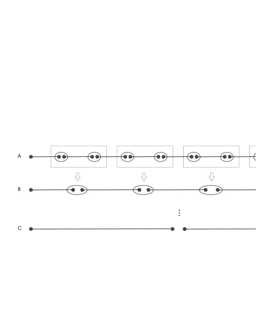
Figure 2: Coarse-graining matrix product states

The quantum coarse–graining procedure where we map two neighboring spins to one new block spin can be fully characterized in terms of the matrices $A$ for the corresponding representatives. These matrices can be conveniently chosen starting from the coarse–grained matrices $\tilde{A}^{(pq)}:=A^{p}A^{q}$ through the singular value decomposition

$$(\tilde{A}^{(pq)})_{\alpha\gamma}=\sum_{l=1}^{\min(d^{2},D^{2})}(U^{\dagger})^{(pq)}_{l}\lambda^{l}(V^{l})_{\alpha\gamma}.$$ (4)

¿From this decomposition we identify the isometry $U$ which selects the representative and the coarse–grained tensor $A^{\prime}$

$$A^{p}\stackrel{{\scriptstyle RG}}{{\longrightarrow}}A^{l}=\lambda^{l}V^{l}.$$ (5)

The advantage of this representative is that the Hilbert space corresponding to the block spins remains bounded above by $D^{2}$ at any step, as it is clear from the decomposition (4). That is, by coarse–graining we do not have to increase the dimension of the spins once we reach $D^{2}$, and therefore, it is possible to perform an exact coarse–graining on finite dimensional matrix product states without any need of truncation! Obviously, the interesting question is now to classify all possible fixed points of this exact renormalization flow.

Before introducing a formalism to characterize those fixed points, let us present some simple examples. The first one is provided by product states (for which $D=1$, $A^{1}=1$ and $A^{k}=0$ for $k=2,\ldots,d$ and $A^{\prime i}=A^{i}$). These are precisely the state obtained for massive theories in their infrared fixed points. A significant further example corresponds to GHZ-like states GHZ . If we take $d=2$ and $A^{0}=|0\rangle\langle 0|,\ A^{1}=|1\rangle\langle 1|$ the RG transformation reads $A^{i}\stackrel{{\scriptstyle RG}}{{\longrightarrow}}A^{\prime i}=A^{i}$ with $U=|0\rangle\langle 00|+|1\rangle\langle 11|$. Those states indeed appear as RG infrared points in e.g. the quantum Ising chain for vanishing external magnetic field LLRV .

Let us now construct a general formalism by which the fixed points can be characterized. In order to circumvent the arbitrariness in the choice of the local bases, we introduce the auxiliary $D^{2}\times D^{2}$ transfer matrix

$$E=\sum_{p=1}^{D}A^{p}\otimes\bar{A}^{p},$$ (6)

where the bar indicates complex conjugation. Note that if we choose $\tilde{A}_{q}=\sum_{p}U_{p}^{q}A^{p}$ with $U$ unitary, we have

$$\tilde{E}=\sum_{q=1}^{D}\tilde{A}^{q}\otimes\tilde{\bar{A}^{q}}=\sum_{p=1}^{D}A^{p}\otimes\bar{A}^{p}=E.$$ (7)

Conversely, the matrix $E$ uniquely defines the matrices $A^{p}$ up to such a local unitary operator, and thus it parameterizes the equivalence class of D-dimensional MPS where all elements of the class are related by local unitary operations note . Furthermore, a RG step corresponds to the simple transformation $E\stackrel{{\scriptstyle RG}}{{\longrightarrow}}E^{\prime}=E^{2}$. Therefore, in order to study the alluded fixed points we just have to characterize the class of possible operators $\{E_{\infty}\}=\{\lim_{n\rightarrow\infty}E^{n}\}$ for some $E$ in the form (6). Since we can always choose the largest eigenvalue of $E$ to be equal to 1 note1 , we just have to characterize all matrices $E$ of the form (6) that have only eigenvalues of magnitude $1$ or $0$ (eigenvalues smaller than 1 will decay exponentially along repeated coarse–graining steps).

In the generic case, the largest eigenvalue of $E$ will be non-degenerate and both its left and right eigenvectors will have maximal Schmidt rank; that is, $E^{\infty}=|\Phi_{R}\rangle\langle\Phi_{L}|$, where the reduced density operators of $\Phi_{L,R}$ are rank $D$ matrices. With the similarity transformation note1 we can always choose $|\Phi_{R}\rangle=\sum_{i=1}^{D}|ii\rangle$ and $|\Phi_{L}\rangle=\sum_{i=1}^{D}\lambda_{i}|ii\rangle$, with $\lambda_{i}>0$. From these eigenvectors we can directly read off the matrices $A^{(pq)}=\sqrt{\lambda_{q}}|p\rangle\langle q|$ with $p,q=1,\ldots,D$. Thus, at the fixed point, the scale–invariant state (representative of the equivalence class) can be written in terms of two auxiliary spins at each point, which are in an entangled state $|\Phi_{L}\rangle$ with its neighbors as shown in Fig. 2(c). This conclusion is very appealing, and has the following consequences:

• All connected correlation functions of the form $\langle O^{i}O^{j}\rangle-\langle O^{i}\rangle\langle O^{j}\rangle$ are exactly zero when $j>i+1$; this is exactly what one expects from a generic state by looking at it in a coarse–grained way: the correlations decay exponentially along the renormalization flow and become zero at the fixed point.

• The entropy of a block of spins of length $L$ is independent of $L$ and is exactly twice the entropy of entanglement of $|\Phi_{R}\rangle$.

• In terms of the picture introduced in VPC04 , coarse–graining turns the virtual underlying spins into real ones but changes the maximally entangled states into $|\Phi_{R}\rangle$.

The qualitative features of the renormalization flow can also be easily understood. For example, an observable that only acts nontrivially on the spins in the center of a block converges exponentially fast to the identity operator times its expectation value; this was indeed expected as observables defined in the middle of a block of length $L$ with $L$ larger than the correlation length should not be able to act nontrivially on the spins far away. On the other hand, the entropy of a block increases by coarse–graining (if we do not rescale the lengths). By the strong subadditivity of the entropy (cf.NielseChuang ) this is even true in general for all translationally invariant states.

As an illustration of the generic case analyzed above, let us consider the ground state of the AKLT Hamiltonian AKLT , for which $A^{p}=\sigma^{p}$ ($p=1..3$) are the Pauli matrices. Some simple algebra shows that $E$ has eigenvalues $3,1,-1,-1$ and hence no degeneracy in the largest eigenvalue. The fixed point is given by the eigenvector corresponding to eigenvalue $3$, namely $E_{i}=|I\rangle\langle I|$ with $|I\rangle=\sum_{i=1}^{2}|ii\rangle$. Hence, it is a dimer of maximally entangled states, i.e., in the language of QI a perfect resource for a quantum repeater. Intriguingly, this is also the exact fixed point of the 1-D cluster state cluster represented by $A^{0}=|0\rangle(\langle 0|+\langle 1|)$ , $A^{1}=|1\rangle(\langle 0|-\langle 1|)$. However, in this case the fixed point is already obtained after one coarse–graining step as the corresponding $E$ contains a nilpotent Jordan block:

$$E_{=}\frac{1}{2}\left(\begin{array}[]{cccc}1&1&1&1\\ 0&0&0&0\\ 0&0&0&0\\ 1&-1&-1&1\end{array}\right)\hskip 14.22636ptE_{cl}^{2}=\sum_{ij}|ii\rangle\langle jj|.$$ (8)

The formalism developed above can also be applied in the case $D\to\infty$. To illustrate that, let us consider an Ising chain with transverse magnetic field or an anisotropic Heisenberg antiferromagnet. In the non–critical regime, their correlation length $\xi$ is finite, which implies that the associated operator $E$ will have a non-degenerate largest eigenvalue ($1/\xi\propto\ln(\lambda_{1}/\lambda_{2})$). Accordingly, the fixed point of the coarse–graining map will therefore consist of a dimer state. The eigenvalues of the reduced density operator of a half-infinite chain are precisely the Schmidt coefficients of the bipartite states making up the dimer. We can in fact determine these coefficients by using the results of Peschel and col. Peschel , who have been able to determine the mentioned reduced density operator exactly. For the Ising model we have

$$\lambda_{(n_{1},n_{2},\cdots n_{\infty})}=\begin{cases}e^{-\epsilon\sum_{j=0}^{\infty}(2j+1)n_{j}}&\lambda<1\\ e^{-\epsilon\sum_{j=0}^{\infty}2jn_{j}}&\lambda>1.\end{cases}$$ (9)

Here $\epsilon=\pi K[(1-\mu^{2})^{1/2}]/K(\mu)$, with $K$ the complete elliptic integral of the 1st kind, $\mu=\min(\lambda,1/\lambda)$, and $n_{j}\in\{0,1\}$. In the case of the noncritical Heisenberg model $H_{XXZ}=\sum_{i}\sigma^{x}_{i}\sigma^{x}_{i+1}+\sigma^{x}_{i}\sigma^{x}_{i+1}+\Delta\sigma^{z}_{i}\sigma^{z}_{i+1}$ with $\Delta>1$, the eigenvalues are as in the Ising case with $\lambda>1$, but with $\epsilon={\rm arccosh}(\Delta)$.

We consider now the full classification of fixed points for the simplest non–trivial case $D=2$. By considering the right eigenvectors of $E$ corresponding to the maximal eigenvalue, we have two possibilities note2 : (a) one of them, say $|\Phi_{R}\rangle$, is entangled; (b) there exists only one eigenvector which corresponds to a product state.

In the first case (a), by using the similarity transformation note we can always take $|\Phi_{R}\rangle=\sum_{i=1}^{2}|ii\rangle$. Using the isomorphism note2 and the full classification of trace preserving completely positive maps acting on a qubit Ruskai one can prove that $E_{\infty}$ has rank $1,4$ or $2$. For the first cases, we recover the generic case studied above or obtain a product state, respectively. When the rank is 2 we obtain $A^{0}=|0\rangle\langle 00|;A^{1}=|1\rangle\langle 11|$, i.e., the GHZ state GHZ studied above.

The situation is more complicated in the second case (b), as this implies that $E$ is not diagonalizable but has a Jordan–block decomposition. Some tedious but straightforward algebra leads to two different possibilities for the fixed points. In the first case the effective Hilbert space is 2-dimensional and

$$A^{0}=\begin{pmatrix}1&0\\ 0&\exp(-i\theta)\end{pmatrix}\hskip 56.9055ptA^{1}=\begin{pmatrix}0&0\\ 1&0\end{pmatrix}.$$ (10)

Note that $A^{0}A^{1}=e^{-i\theta}A^{1}$ and that $A^{1}$ is nilpotent; this immediately implies that the state, when written in the computational basis, consists of terms like $|00\cdots 010\cdots 0\rangle$ where at most one $|1\rangle$ appears. When $\theta=0$ we recover the well–known $W$-state W , which is indeed scale invariant. In the second case of Jordan fixed points, the spins have effective support on a Hilbert space of dimension 3 (but 2 when $\cos(\alpha)=1$), and a possible decomposition is given by

$$\begin{split}A^{0}=&\begin{pmatrix}0&0\\ \cos(\alpha)\sin(\beta)&e^{i\theta}\end{pmatrix}\hskip 14.22636ptA^{1}=\begin{pmatrix}0&0\\ \sin(\alpha)&0\end{pmatrix}\\ &A^{2}=\begin{pmatrix}e^{-i\theta}&0\\ \cos(\alpha)\cos(\beta)&0\end{pmatrix}.\end{split}$$ (11)

As $A^{0}A^{1}\propto A^{1},A^{1}A^{2}\propto A^{2},A^{0}A^{2}\propto A^{1},A^{1}A^{0}=0,A^{2}A^{1}=0,A^{2}A^{0}=0$, the state will be a superposition of terms of the form $|00\cdots 0122\cdots 2\rangle$. Therefore these scale-invariant states represent linear combination of domain walls.

For the case $D=2$ this completes the classification of all fixed points, which remarkably correspond to almost all well-studied multipartite states encountered in QI. We note that in the thermodynamic limit case (b) in the classification is redundant in the sense that W and product state as well as domain wall and GHZ state become then locally indistinguishable. A distinction can, however, be relevant from a QI perspective, where it is more natural to carry out only a finite number of coarse–graining steps which enlarge the region of local accessibility only to a physically reasonable vicinity. In this context the system to be transformed can thus be finite.

For $D>2$ a coarse classification of the fixed points can be given by their possible decompositions into ergodic states and their periodic components discussed in Fannes .

Finally, let us mention that we have concentrated here on 1D systems, since in that case MPS give a very useful description. Fortunately, the analogue of MPS in higher dimensions has been recently put forward PEPS , which may allow us to extend the analysis introduced here to two and three spatial dimensions.

Let us conclude with a comment on irreversibility of RG flows. Our RG transformation defined on finite matrix product states incorporates unitarity in a natural way at variance with other approaches. Moreover, the eigenvalues of $E^{2}$ are smaller than the ones of $E$. RG flows will inevitably eliminate all the eigenvalues smaller than 1, which can be phrased as irrelevant pieces of the state. A careful treatment of irreversibility of RG flows should incorporate the infinite dimensional case, associated to conformal field theories, and the discussion of degeneracy in the final relevant Hilbert space.

Work supported by DFG (SFB 631), European projects (RESQ, TOPQIP, CONQUEST), Kompetenznetzwerk der Bayerischen Staatsregierung Quanteninformation and MCyT.

References

- (1) K.G. Wilson, Rev. Mod. Phys. 47, 773 (1975).
- (2) S. White, Phys. Rev. Lett. 69, 2863 (1992); U. Schollwöck, cond-mat/0409292.
- (3) I. Affleck et al., Commun. Math. Phys. 115, 477 (1988).
- (4) M. Fannes, B. Nachtergaele, R.F. Werner, Comm. Math. Phys. 144, 443 (1992).
- (5) L. Kadanoff, Physics 2, 263 (1966); Rev. Mod. Phys. 39, 395 (1967).
- (6) G. Vidal et al., Phys. Rev. Lett. 90, 227902 (2003); J.I. Latorre, E. Rico, G. Vidal, Quant. Inf. and Comp. 4 48, (2004).
- (7) F. Verstraete, D. Porras, J.I. Cirac, cond-mat/0404706.
- (8) D.M. Greenberger, M. Horne, A. Zeilinger, Bell’s theorem, Quantum Theory, and Conceptions of the Universe ed. M. Kafatos, Kluwer (1989).
- (9) J.I. Latorre et al., quant-ph/0404120.
- (10) H.J. Briegel, R. Raussendorf Phys. Rev. Lett. 86, 910 (2001).
- (11) For a given invertible matrix, , and a number , the matrices and define the same state, up to normalization.
- (12) According to note , and provide the same description of the state. We can use this fact to demand certain properties of .
- (13) Matrices can be isomorphically mapped into completely positive maps, , which act as follows: . Thus, we can use the knowledge of the classification of those maps Ruskai in order to classify the structure of .
- (14) M.B. Ruskai, S. Szarek, E. Werner, Lin. Alg. Appl. 347, 159 (2002).
- (15) M. Nielsen and I. Chuang, Quantum computation and quantum information, Cambridge Univ. Press (2000).
- (16) I. Peschel, M. Kaulke, O. Legeza, Ann. Physik (Leipzig) 8, 153 (1999).
- (17) W. Dür, G. Vidal, J.I. Cirac Phys. Rev. A 62, 062314 (2000).
- (18) F. Verstraete, J.I. Cirac, cond-mat/0407066.