Physical implementation of entangling quantum measurements

Abstract

We clarify the microscopic structure of the entangling quantum measurement superoperators and examine their possible physical realization in a simple three-qubit model, which implements the entangling quantum measurement with an arbitrary degree of entanglement.

I Introduction

In quantum information theory, generalized description of most important quantum transformations, which extend the class of unitary transformations lying in the foundations of quantum theory of dynamically closed quantum systems a , plays very important role b . Particulary, the resulting transformation in a system describing only the measured object to which we apply the standard quantum measurement can be written in a form of so called projective measurement superoperator:

$${\cal M}_{P}=\sum\mathop{\left|k\right\rangle}\nolimits\mathop{\left\langle k\right|}\nolimits\odot\mathop{\left|k\right\rangle}\nolimits\mathop{\left\langle k\right|}\nolimits,$$ (1)

where the $k$-terms of the sum describe the normalized positive superoperator measure (PSM), which is represented here by the orthogonal projection superoperators of the form

$${\cal E}_{k}=\mathop{\left|k\right\rangle}\nolimits\mathop{\left\langle k\right|}\nolimits\odot\mathop{\left|k\right\rangle}\nolimits\mathop{\left\langle k\right|}\nolimits,\quad\sum{\rm Tr}\,{\cal E}_{k}={\rm Tr}\,\odot.$$

Respectively, $\sum{\cal E}_{k}^{+}\hat{I}=\sum\mathop{\left|k\right\rangle}\nolimits\mathop{\left\langle k\right|}\nolimits=\hat{I}$ (see, for instance, c ). The substitution symbol $\odot$ is to be substituted by a transformed operator, which is simply the density matrices in our case d ; e ; index $k$ enumerates the eigen vectors of the measured physical variable, which is described by the operator $\hat{A}=\sum\lambda_{k}\mathop{\left|k\right\rangle}\nolimits\mathop{\left\langle k\right|}\nolimits$ in the Hilbert space $H_{A}$ of the measured object. The generalized measurement, which is carried out in the extended space $H_{A}\otimes H_{a}$ of the initial and auxiliary systems, is described by the PSM of the general form ${\cal E}_{k}=\hat{F}_{k}\odot\hat{F}_{k}^{+}$ in the linear space of operators in $H_{A}$. The corresponding classical probabilistic measure on the spectrum of physically possible values $\lambda_{k}$ of the operator $\hat{A}$ is described by the linear functional $\hat{\rho}_{A}\to P(k)={\rm Tr}\,\hat{E}_{k}\hat{\rho}_{A}$, which is determined by a non-orthogonal expansion of the unit operator f

$$\hat{E}_{k}=\hat{F}_{k}^{+}\hat{F}_{k},\quad\sum\hat{E}_{k}=\hat{I},$$

which is the positive operator valued measure (POVM) g .

Due to the progress in quantum state engineering made over last decades h , the commonly accepted concept of quantum measurement as a projective transformation has been essentially revised. It includes now various types of measurements, e.g., the measurement that provides the measured information in a form of quantum entanglement between the apparatus and the measured object. By contrast with the classical theory, the equality $A\equiv B$, which means the coincidence of the physical values $A$ and $B$ for all their possible values $\lambda$, can be realized now differently. This equality does not prevent arbitrary relations between the phases $\varphi_{\lambda}$ corresponding to the eigen wave-functions $\Psi_{\lambda}$ implementing the equality $A=B=\lambda$. Therefore, the standard quantum measurement implies complete absence of the phase correlations, whereas the completely coherent measurement implies the defined set of phases.

The respective most general abridged notation for the ideal quantum measurement transformation in the object–apparatus system is given by the entangling quantum measurement superoperator e . This entangling quantum measurement can be considered as a combination of the completely coherent measurement, which provides the measurement results in a form of quantum entanglement between the apparatus and the object, and additional transformation dephasing the states of the apparatus

$${\cal D}=\sum_{ij}R_{ij}\mathop{\left|i\right\rangle}\nolimits\mathop{\left\langle i\right|}\nolimits\odot\mathop{\left|j\right\rangle}\nolimits\mathop{\left\langle j\right|}\nolimits$$

with the positive entanglement matrix $R\geq 0$ with the diagonal elements $R_{ii}\equiv 1$. The entangling quantum measurement is an intermediate transformation between the identity superoperator transformation ${\cal I}=\sum_{ij}\mathop{\left|i\right\rangle}\nolimits\mathop{\left\langle i\right|}\nolimits\odot\mathop{\left|j\right\rangle}\nolimits\mathop{\left\langle j\right|}\nolimits$, which corresponds to the case of $R_{ij}\equiv 1$, and the projective measurement transformation (1), which corresponds to the diagonal matrix $R_{ij}=\delta_{ij}$.

Definition of quantum measurement considered in Ref. e is based on the natural interpretation of the quantum measurement as the transformation, which is invariant with regard to the initial state of the apparatus. However, in a wide range of experimental situations h ; i ; j ; k the quantum measurement transformations are applied to a bipartite system when the initial state of one of the subsystems is explicitly known (it can be, for example, the ground or specially prepared quantum state of an atom or non-excited resonator mode). Both cases can be described with the superoperators of a specialized type, which instead of the complete mapping (object+apparatus) $\to$ (object+apparatus) define the mapping (object) $\to$ (object+apparatus). It is worth to note here that for a potentially capable experimental realization of the measurement transformations considering appropriate mathematical representation of a specific physical situation is of prime importance.

In this work, we elucidate possibility of physical implementation of an entangling measurement. The general theory is illustrated on example of two-level models, which describe in an idealized form some features of quantum transformations that are typical, for instance, for the experiments with trapped atoms.

In Sec. II we give precise mathematical definitions of the extended superoperators and discuss how they can be applied to the various types of the ideal quantum measurement. Also, we give physical interpretation of the coherent information, which is bound to the entangling quantum measurement. Unitary implementations of the extended superoperators in connection with the experimental specificity of physical implementations of non-reversal transformations are considered in Sec. III. In Sec. IV we consider specific matrix representations in application to the extended superoperators technique. In Sec. V we specify a unitary realization of the entangling measurement in a simple three-qubit model, which implements the entangling quantum measurement with an arbitrary degree of entanglement.

II Mathematical definitions of extended superoperators

In order to clarify physical implementation of the measurement transformations, its mathematical representation has to have a clear and simple form. Extended superoperators perfectly fit this purpose and their definitions are considered below in detail.

Let us consider a superoperator transformation ${\cal S}$ in a bipartite system $A$+$B$, which we apply to the density matrix $\hat{\rho}_{AB}=\hat{\rho}_{A}\otimes\hat{\rho}_{B}^{0}$ of this system in the Hilbert space $H_{A}\otimes H_{B}$, where $\hat{\rho}_{B}^{0}$ is an arbitrary chosen fixed state. Then, the result of this superoperator transformation is simply a map $\mathbb{C}(H_{A})\to\mathbb{C}(H_{A}\otimes H_{B})$ of the operators algebra in $H_{A}$ onto the corresponding algebra in $H_{A}\otimes H_{B}$ and can be written in a symbolic representation as

$${\cal E}={\cal S}(\odot\otimes\hat{\rho}_{B}^{0}),$$ (2)

where the substitution symbol $\odot$ should be substituted by single transformed operator $\hat{\rho}_{A}$. By contrast with ${\cal S}$, the extended superoperator ${\cal E}$ has an “extended” in comparison with the input $\hat{\rho}_{A}$ space with the elements $\hat{\rho}_{AB}={\cal E}\hat{\rho}_{A}$.

If the result of the superoperator transformation does not depend on $\hat{\rho}_{B}^{0}$, i.e., ${\cal E}={\cal E}_{0}\equiv{\cal S}(\odot\otimes\hat{\rho}_{B})$ for all $\hat{\rho}_{B}$, we have another special case, when the superoperator transformation ${\cal S}$ can be described entirely with the extended superoperator (2). The corresponding structure of such invariant superoperator has the form:

$${\cal S}=\sum_{ij}\Bigl{(}{\cal S}^{A}_{ij}\,\odot_{A}\Bigr{)}\otimes\Bigl{(}\mathop{\left|i\right\rangle}\nolimits\mathop{\left\langle j\right|}\nolimits{\rm Tr}\,\odot_{B}\Bigr{)},$$ (3)

where the trace operation makes the result independent of an initial state of the system $B$.

The extended superoperator (2) may be treated as a “hybrid” superoperator transformation over the variables of the system $A$ and the density matrix operator over the variables of the system $B$. Respectively, tracing the extended superoperator over the variables of the system $B$ results in a regular superoperator ${\cal S}_{A}={\rm Tr}_{B}{\cal E}$, which maps algebra $\mathbb{C}(H_{A})$ onto itself. The relation ${\cal S}_{A}\to{\cal E}$ can be considered as an extension of the value area of the superoperator, which is related to the concrete definition of the respective physical transformation in an open system in the symbolic representation form (2).

Apparently, the extended superoperator (2) has the same specificity for all superoperators properties—the complete positivity and normalization. In case of $d$-dimensional Hilbert spaces $H_{A}$, $H_{B}$, the extended superoperator can be represented in the matrix representation by the rectangular matrices of $d^{4}\times d^{2}$-dimension, whereas a regular superoperator ${\cal S}$ is described by rectangular matrices of $d^{4}\times d^{4}$-dimension. In a specific case of two qubits, these are $16\times 4$ and $16\times 16$ matrices, respectively. Keeping this in mind, one can essentially reduce complexity of the respective calculations performing them in terms of the extended superoperators, when it is possible.

With the help of an orthogonal basis $\mathop{\left|k\right\rangle}\nolimits$ in $H_{A}$ the extended superoperator (2) has the following, as one can easily see, most generalized form:

$${\cal E}=\sum\hat{s}_{kl}\mathop{\left\langle k\right|}\nolimits\odot\mathop{\left|l\right\rangle}\nolimits,$$ (4)

where $\hat{s}_{kl}$ is the set of operators in $H_{A}\otimes H_{B}$, which satisfy the above mentioned complete positivity and normalization conditions.

From the properties of the extended superoperators it is also follows that more than one regular superoperator can correspond to the extended one. Also, possibility of physical implementation of the extended superoperator ${\cal E}$, which satisfies the complete positivity condition, readily follows from the general criterion of physical implementation of a regular superoperator b and it is enough to have only the existence proof of a complete positive superoperator ${\cal S}$ and density matrix $\rho_{B}^{0}$, related to ${\cal E}$ according to the Eq. (2).

Let us consider the entangling measurement superoperator:

$${\cal M}=\sum_{ijm}R_{ij}\mathop{\left|i\right\rangle}\nolimits\mathop{\left|i\right\rangle}\nolimits\mathop{\left\langle j\right|}\nolimits\mathop{\left\langle j\right|}\nolimits\mathop{\left\langle m\right|}\nolimits\mathop{\left\langle i\right|}\nolimits\odot\mathop{\left|j\right\rangle}\nolimits\mathop{\left|m\right\rangle}\nolimits$$ (5)

with the entanglement matrix $(R_{ij})\geq 0,R_{ii}\equiv 1$ e , which is a particular case of the invariant superoperator (3). The resulted state after its action does not depend on an initial state of the system $B$ and with the help of (4) the corresponding extended entangling measurement superoperator has the form:

$${\cal E}_{M}=\sum_{ij}\bigl{(}R_{ij}\mathop{\left|i\right\rangle}\nolimits\mathop{\left|i\right\rangle}\nolimits\mathop{\left\langle j\right|}\nolimits\mathop{\left\langle j\right|}\nolimits\bigr{)}\mathop{\left\langle i\right|}\nolimits\odot\mathop{\left|j\right\rangle}\nolimits.$$ (6)

Here, the resulted state $\hat{\rho}_{AB}$ is represented only via the cloned basis states $\mathop{\left|i\right\rangle}\nolimits\mathop{\left|i\right\rangle}\nolimits$, which means that the quantum measurement was an ideal one. Also, a fact that $R_{ij}\neq 1$ at $i\neq j$ is an evidence that the measurement is an incoherent one. Even in the case of complete coherency, $R_{ij}\equiv 1$, when the entangling superoperator (5) describes cloning transformation of the basis states,

$${\cal C}=\sum_{ijm}\mathop{\left|i\right\rangle}\nolimits\mathop{\left|i\right\rangle}\nolimits\mathop{\left\langle j\right|}\nolimits\mathop{\left\langle j\right|}\nolimits\mathop{\left\langle m\right|}\nolimits\mathop{\left\langle i\right|}\nolimits\odot\mathop{\left|j\right\rangle}\nolimits\mathop{\left|m\right\rangle}\nolimits,$$ (7)

it is non-reversal because information of an initial state of the apparatus $\hat{\rho}_{B}$ is completely ignored.

The extended superoperator for the entangling measurement can be additionally extended in a way to clarify the quantum nature of the entanglement matrix. This can be readily done by introducing additional internal degrees of freedom in $H_{D}$ space that are responsible for the dephasing effects, i.e., in the form of the extended superoperator $A\to(A{+}B{+}D)$ of the form:

$${\cal E}_{M}=\sum_{ij}\mathop{\left|i\right\rangle}\nolimits\mathop{\left|i\right\rangle}\nolimits\mathop{\left|\mathop{\left|i\right\rangle}\nolimits\right\rangle}\nolimits\mathop{\left\langle\mathop{\left\langle j\right|}\nolimits\right|}\nolimits\mathop{\left\langle j\right|}\nolimits\mathop{\left\langle j\right|}\nolimits\mathop{\left\langle i\right|}\nolimits\odot\mathop{\left|j\right\rangle}\nolimits,$$ (8)

where internal degrees of freedom are in the double brackets and, generally, are non-orthogonal and are described by the scalar product $\left<\mathop{\left\langle i\left|j\right.\right\rangle}\nolimits\right>=R_{ij}$, which ensures coincidence with Eq. (6) after averaging over states in $H_{D}$. Such representation of the extended superoperator clarifies physical essence of the dephasing processes as modulation of the states $\mathop{\left|i\right\rangle}\nolimits\mathop{\left|i\right\rangle}\nolimits$ $H_{A}\otimes H_{B}$ by the internal states $\mathop{\left|\mathop{\left|i\right\rangle}\nolimits\right\rangle}\nolimits$, which define an additional quantum “phase” depending, in general, on $i$.

The states of the micro-variables of the apparatus are described in accordance with Eq. (8) by the partial density matrices:

$$\hat{\rho}_{D}=\sum_{i}p_{i}\mathop{\left|\mathop{\left|i\right\rangle}\nolimits\right\rangle}\nolimits\mathop{\left\langle\mathop{\left\langle i\right|}\nolimits\right|}\nolimits,$$ (9)

where probabilities $p_{i}=\mathop{\left\langle i\right|}\nolimits\hat{\rho}_{A}\mathop{\left|i\right\rangle}\nolimits$ are determined only by the density matrix of the measuring object and by the eigen basis of the measuring physical variable $\hat{A}=\sum_{i}\lambda_{i}\mathop{\left|i\right\rangle}\nolimits\mathop{\left\langle i\right|}\nolimits$. In case of the standard non-coherent measurement it coincides (at a properly chosen basis set) with the reduced density matrix of the object

$$\hat{\rho}_{\rm red}=\sum_{i}\mathop{\left|i\right\rangle}\nolimits\mathop{\left\langle i\right|}\nolimits\hat{\rho}_{A}\mathop{\left|i\right\rangle}\nolimits\mathop{\left\langle i\right|}\nolimits.$$

In the opposite case of the completely coherent measurement, $\mathop{\left|\mathop{\left|i\right\rangle}\nolimits\right\rangle}\nolimits\equiv\mathop{\left|\mathop{\left|0\right\rangle}\nolimits\right\rangle}\nolimits$, we have $\hat{\rho}_{D}=\mathop{\left|\mathop{\left|0\right\rangle}\nolimits\right\rangle}\nolimits\mathop{\left\langle\mathop{\left\langle 0\right|}\nolimits\right|}\nolimits$ and, respectively, the microstates entropy equals to zero.

In this connection, it is worth to note that the zero microstates entropy does not prevent manifestation of physically essential macroscopic fluctuations in the system. Besides a subset of physical variables for which $\mathop{\left|\mathop{\left|0\right\rangle}\nolimits\right\rangle}\nolimits$ is the eigenstate, there is an “overwhelming majority” (this qualitative characteristic can be readily concretized mathematically) of other variables that results in quantum fluctuations, of perfectly macroscopic character inclusive. It is clear, in principle, that any quantum state of a macro-object can be considered as a pure state at the microscopic level in the frame of sufficiently complete microscopic model, which includes all physical subsystems the object interacts with.

The coherent information l or preserved entanglement m ; n

$$I_{c}=S[\hat{\rho}_{B}]-S[\hat{\rho}_{AB}]$$

corresponding to the entangling measurement can be expressed via the entropy of the measured variables and the entropy of the dephased micro-subsystem. To do that, we should keep in mind that due to the ideal character of the measurement, the marginal density matrix of the measuring variables coincides with the reduced one of the object. Also, because the only source of decoherence is in the subsystem $D$ in transformation (8), the entropy of the joint density matrix $\hat{\rho}_{AB}$ coincides with the entropy of this dephasing subsystem. As a result we get

$$I_{c}=S[\rho_{\rm red}]-S[\hat{\rho}_{D}].$$ (10)

i.e., by contrast with the general case, in the form of always positive difference between entropy of the reduced by the measurement state of the object and entropy of the apparatus microstates. The latter is inevitably less than the entropy of the resulted state of the measured object, because otherwise it will not meet the ideal measurement requirements according to which a macro-variable describing the result of the measurement does not show classical fluctuations. Mathematically, this means that $\hat{k}_{B}\equiv\hat{k}_{A}$, where $\hat{k}_{B}=\sum_{i}i{\mathop{\left|i\right\rangle}\nolimits}_{B}{\mathop{\left\langle i\right|}\nolimits}_{B}$, $\hat{k}_{A}=\sum_{i}i{\mathop{\left|i\right\rangle}\nolimits}_{A}{\mathop{\left\langle i\right|}\nolimits}_{A}$, and respective to each $\mathop{\left|i\right\rangle}\nolimits$ states exhibit only quantum uncertainty, which is due to the nonorthogonality of the microstates $\mathop{\left|\mathop{\left|i\right\rangle}\nolimits\right\rangle}\nolimits$. Therefore, the microstates entropy reaches the entropy $S[\hat{\rho}_{\rm red}]$ of the measuring variable $\hat{k}_{A}$ (and, simultaneously, $\hat{k}_{B}$) only for the case of “maximally independent”, orthogonal, microstates $\mathop{\left|\mathop{\left|i\right\rangle}\nolimits\right\rangle}\nolimits$. In this case, the coherent information (10) vanishes.

III Unitary implementation of the extended superoperators

The non-reversal, invariant in respect to the apparatus’ state, cloning superoperator (7) can be presented in the form ${\cal C}={\cal U}_{C}{\cal R}_{0}$ as a superposition of the superoperator ${\cal R}_{0}={\cal I}_{A}\otimes\mathop{\left|1\right\rangle}\nolimits\mathop{\left\langle 1\right|}\nolimits\sum_{m}\mathop{\left\langle m\right|}\nolimits\odot_{B}\mathop{\left|m\right\rangle}\nolimits$, which sets an initial state of the system $B$ into the given pure state $\mathop{\left|1\right\rangle}\nolimits\mathop{\left\langle 1\right|}\nolimits$, and the respective unitary cloning superoperator ${\cal U}_{C}=U_{C}\odot_{AB}U^{-1}_{C}$, in which the unitary transformation $U_{C}$ $H_{A}\otimes H_{B}$ has the form:

$$\mathop{\left|i\right\rangle}\nolimits\mathop{\left|1\right\rangle}\nolimits\to\mathop{\left|i\right\rangle}\nolimits\mathop{\left|i\right\rangle}\nolimits,\quad\mathop{\left|i\right\rangle}\nolimits\mathop{\left|j\neq 1\right\rangle}\nolimits\to\mathop{\left|k_{ij}\right\rangle}\nolimits\mathop{\left|l_{ij}\right\rangle}\nolimits,$$ (11)

where two arbitrary indices $k_{ij}$, $l_{ij}$ obey the only constraint $k_{ij}\neq l_{ij}$. This transformation is illustrated in Fig. 1 on example of two two-level systems. The extended superoperator ${\cal E}_{C}={\cal C}\bigl{(}\odot_{A}\otimes\mathop{\left|1\right\rangle}\nolimits\mathop{\left\langle 1\right|}\nolimits\bigr{)}$ corresponding to ${\cal C}$ can be explicitly represented via the unitary transformation in the bipartite system:

$${\cal E}_{C}=U_{C}\bigl{(}\odot_{A}\otimes\mathop{\left|1\right\rangle}\nolimits\mathop{\left\langle 1\right|}\nolimits\bigr{)}U^{-1}_{C}.$$ (12)

From experimental point of view, it is well known that reversibility of a physical transformation, which corresponds to the unitarity, is of great importance for a potential implementation. This is because the reversibility is, generally, connected with the exchange of energy and respective recoil momentum, which for the cold atoms in traps, for instance, could lead to uncontrolled processes, up to loosing atoms from the trap k . However, such effects can be avoided if we apply a non-reversal setting of the entanglement matrix ${\cal R}_{0}$ and, respectively, an invariant cloning transformation ${\cal C}$ to the previously set equilibrium state $\mathop{\left|1\right\rangle}\nolimits\mathop{\left\langle 1\right|}\nolimits$.

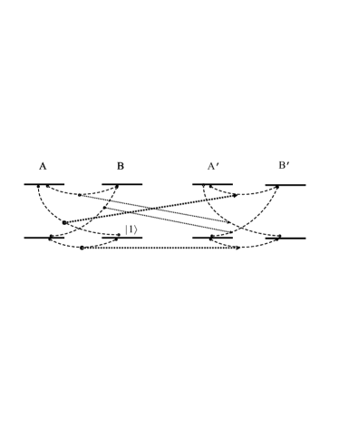
Figure 1: Unitary representation ${\cal U}_{C}$ of the extended cloning superoperator (12), which is defined on the basis of eigenstates of two two-level systems $A$ and $B$. Basis states of the joint $A+B$ system (dashed lines), which exist after setting the system $B$ with the transformation ${\cal R}_{0}$ into the ground state $\mathop{\left|1\right\rangle}\nolimits$, are transferred into the states $\mathop{\left|i\right\rangle}\nolimits\mathop{\left|i\right\rangle}\nolimits$ (bold dotted arrows), whereas the rest of the states are transferred into the states $\mathop{\left|i\right\rangle}\nolimits\mathop{\left|j\neq i\right\rangle}\nolimits$ (thin dotted arrows).

Let us now prove that the extended superoperator of entangling measurement (8) can be physically implemented with the help of unitary transformation immediately in the system of object–apparatus–internal variables, i.e., in $H_{A}\otimes H_{B}\otimes H_{D}$. Construction of such a transformation splits into two steps.

First, we construct a unitary map ${\cal U}_{C}$ in the system object–apparatus of the form of Eq (11) and take into account that after this transformation in $H_{A}\otimes H_{B}$ there will be only cloning states $\mathop{\left|i\right\rangle}\nolimits\mathop{\left|i\right\rangle}\nolimits$.

Then, after selecting an arbitrary initial state $\mathop{\left|\mathop{\left|0\right\rangle}\nolimits\right\rangle}\nolimits$ in $H_{D}$, it is sufficient to construct in the subsystem $H_{B}\otimes H_{D}$ a unitary partial entanglement operator $U_{E}$, which includes, in general case, dephasing effects and fits the following relations

$$U_{E}\mathop{\left|i\right\rangle}\nolimits\mathop{\left|\mathop{\left|0\right\rangle}\nolimits\right\rangle}\nolimits=\mathop{\left|i\right\rangle}\nolimits\mathop{\left|\mathop{\left|i\right\rangle}\nolimits\right\rangle}\nolimits$$ (13)

for all $i=1,\dots,d$. Taking into account that vectors $\mathop{\left|i\right\rangle}\nolimits$ are orthogonal to each other, such map preserves initial metric, i.e., orthonormalization of the transformed vectors. This guarantees that there is a space, which maps $d^{2}-d$ vectors $\mathop{\left|i\right\rangle}\nolimits\mathop{\left|\mathop{\left|j\neq i\right\rangle}\nolimits\right\rangle}\nolimits$ in a respective arbitrary chosen basis set in a subspace orthogonal to the $d$-mensional subspace of vectors $\mathop{\left|i\right\rangle}\nolimits\mathop{\left|\mathop{\left|i\right\rangle}\nolimits\right\rangle}\nolimits$. Two-dimensional example of such a unitary transformation is illustrated in Fig. 2.

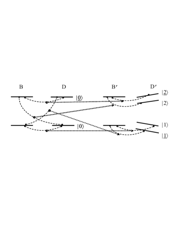
Figure 2: Unitary transformation $U_{E}$ for partial entanglement of two qubits, where $\{\mathop{\left|0\right\rangle}\nolimits,\mathop{\left|\underline{0}\right\rangle}\nolimits\}$, $\{\mathop{\left|1\right\rangle}\nolimits,\mathop{\left|\underline{1}\right\rangle}\nolimits\}$, and $\{\mathop{\left|2\right\rangle}\nolimits,\mathop{\left|\underline{2}\right\rangle}\nolimits\}$ designate three orthogonal bases in $H_{D}$ arbitrary rotated to each other.

With the help of equations (13) and (11) one can easily see that the extended superoperator of entangling measurement (8) can be written in a form of superposition of unitary transformations acting on the object density matrices at the initial state $\mathop{\left|1\right\rangle}\nolimits\mathop{\left|\mathop{\left|0\right\rangle}\nolimits\right\rangle}\nolimits$ of the apparatus and its internal variables:

$${\cal E}_{M}=\bigl{(}{\cal I}_{A}\otimes{\cal U}_{E}\bigr{)}\bigl{(}{\cal U}_{C}\otimes{\cal I}_{D}\bigr{)}\bigl{(}\odot\otimes\mathop{\left|1\right\rangle}\nolimits\mathop{\left\langle 1\right|}\nolimits\otimes\mathop{\left|\mathop{\left|0\right\rangle}\nolimits\right\rangle}\nolimits\mathop{\left\langle\mathop{\left\langle 0\right|}\nolimits\right|}\nolimits\bigr{)}.$$ (14)

In a case of pure cloning, i.e., without any dephasing, the unitary superoperator ${\cal U}_{E}$ is represented by the identity superoperator (one should also take into account freedom in selection the basis states, which leads to further generalization or simplification due to the corresponding unitary transformation of the form $\sum_{j}e^{i\varphi_{j}}\mathop{\left|j\right\rangle}\nolimits\mathop{\left\langle j\right|}\nolimits$).

IV Matrix representation of the extended superoperators

From practical point of view, one of the most useful variants of the matrix representation of the extended superoperators $A\to A{+}B$ is based on the fixed linear basis $\hat{e}_{k}^{A}$ for determining the input states $\hat{\rho}_{A}=\sum\rho_{n}\hat{e}_{n}^{A}$. The corresponding representation of the resulting density matrix $\hat{\rho}_{AB}=\sum\rho_{n}{\cal E}\hat{e}_{n}^{A}$ is determined then by the set of basis operators:

$$\hat{\cal E}_{n}={\cal E}\hat{e}_{n}^{A},\quad\hat{\rho}_{AB}=\sum\rho_{n}\hat{\cal E}_{n}.$$

Thus, the extended superoperators are represented by the operator set $\hat{\cal E}_{n}$, $n=1,\dots,d^{2}$ in the space $H_{A}\otimes H_{B}$. Operators $\hat{\cal E}_{n}$, in their turn, can be represented by the corresponding matrices of $d^{2}\times d^{2}$-dimensions (or by the matrices of highest dimension in case of additionally extended space $H_{B}$).

One can clearly see that positivity of the extended operator ${\cal E}\to\hat{\cal E}_{n}$ corresponds to the positivity of $\hat{\cal E}_{n}$ in a positive basis $\hat{e}_{n}^{A}$.

Representation of the unitary extended superoperator in case of pure initial states $\hat{\rho}_{B}^{0}=\mathop{\left|1\right\rangle}\nolimits\mathop{\left\langle 1\right|}\nolimits$ reduces simply to a set of orthogonal wave-functions in $H_{A}\otimes H_{B}$. Really, for the two-indices symbolic representation ${\cal E}=\sum U\bigl{(}\mathop{\left\langle k\right|}\nolimits\odot\mathop{\left|l\right\rangle}\nolimits\otimes\mathop{\left|1\right\rangle}\nolimits\mathop{\left\langle 1\right|}\nolimits\bigr{)}U^{-1}$ we receive in the basis $\mathop{\left|k\right\rangle}\nolimits\mathop{\left\langle l\right|}\nolimits$ the following matrix representation: $\hat{\cal E}_{kl}=\Psi_{k}\Psi_{l}^{+}$, where $\Psi_{k}=U\bigl{(}\mathop{\left|k\right\rangle}\nolimits\mathop{\left|1\right\rangle}\nolimits\bigr{)}$ is an arbitrary, in general case, set of $d$ orthogonal vectors in a $d\times d$-dimensional space. In particulary, for the considered above two-dimensional unitary cloning transformation in accordance with the transformation (13) it is represented by a pair of four-dimensional wave-functions in the right side of the equation, which in the basis $\mathop{\left|i\right\rangle}\nolimits\mathop{\left|j\right\rangle}\nolimits$ are described by the rectangular matrix $d\times d^{2}$ of the form:

$$\left(\Psi_{k}\right)=\left(\begin{array}[]{cccc}1&0&0&0\\ 0&0&0&1\end{array}\right).$$ (15)

Here, the coincidence of the states of the subsystems $A$ and $B$ in bipartite states $\Psi_{1}=\mathop{\left|1\right\rangle}\nolimits\mathop{\left|1\right\rangle}\nolimits$, $\Psi_{2}=\mathop{\left|2\right\rangle}\nolimits\mathop{\left|2\right\rangle}\nolimits$ provides an evidence of the clonal character of the resulting state. Such dimension-saving symbolic representations are especially effective for implementation of the calculations with the help of computer algebra, that perform linear transformations with respective degenerate multidimensional density matrices $\Psi_{k}\Psi_{l}^{+}$ without any visible technical problems.

V Physical implementation of the entangling measurement in a system of three qubits

In this section, we analyze an explicit mathematical form of the transformation, which can be used for a possible experimental implementation of the specific realization of the extended superoperator of the entangling quantum measurement described in Sec. III. A system of two two-level atoms in a resonator could serve as a physical example for such an experimental implementation. It can be well modelled by a three-qubit system in which qubits $A$ and $B$ correspond to the two-level atoms in the resonator and third qubit, $D$, describes the states of the resonator mode of electromagnetic field, both vacuum and one-photon.

The transformation ${\cal U}_{C}$ is given by Eq. (11) and we should only specify the entangling superoperator ${\cal U}_{D}$, which in accordance with relation (13) could be specifically defined by the map

$$\begin{array}[]{lcl}\mathop{\left|1\right\rangle}\nolimits\mathop{\left|\mathop{\left|0\right\rangle}\nolimits\right\rangle}\nolimits&\to&\mathop{\left|1\right\rangle}\nolimits\mathop{\left|\mathop{\left|1\right\rangle}\nolimits\right\rangle}\nolimits,\\ \mathop{\left|2\right\rangle}\nolimits\mathop{\left|\mathop{\left|0\right\rangle}\nolimits\right\rangle}\nolimits&\to&\mathop{\left|1\right\rangle}\nolimits\mathop{\left|\mathop{\left|2\right\rangle}\nolimits\right\rangle}\nolimits,\\ \mathop{\left|1\right\rangle}\nolimits\mathop{\left|\mathop{\left|\underline{0}\right\rangle}\nolimits\right\rangle}\nolimits&\to&\mathop{\left|1\right\rangle}\nolimits\mathop{\left|\mathop{\left|\underline{1}\right\rangle}\nolimits\right\rangle}\nolimits,\\ \mathop{\left|2\right\rangle}\nolimits\mathop{\left|\mathop{\left|\underline{0}\right\rangle}\nolimits\right\rangle}\nolimits&\to&\mathop{\left|2\right\rangle}\nolimits\mathop{\left|\mathop{\left|\underline{2}\right\rangle}\nolimits\right\rangle}\nolimits,\end{array}$$ (16)

where underlining marks the vectors orthogonal to the initial ones. The entanglement matrix in this case has all diagonal elements equal to unit and the only off-diagonal element $R_{12}=R_{21}^{*}=\left<\mathop{\left\langle 1\left|2\right.\right\rangle}\nolimits\right>=q$, which does not equal to unit. Transformation for the last pair of vectors can vary from shown above by an arbitrary unitary transformation in the subspace of the respective output pair of the states $\mathop{\left|1\right\rangle}\nolimits\mathop{\left|\mathop{\left|\underline{1}\right\rangle}\nolimits\right\rangle}\nolimits$, $\mathop{\left|2\right\rangle}\nolimits\mathop{\left|\mathop{\left|\underline{2}\right\rangle}\nolimits\right\rangle}\nolimits$.

Combining transformations ${\cal U}_{C}$ and ${\cal U}_{D}$, we receive the resulting unitary map $U_{CD}=\bigl{(}\hat{I}_{A}\otimes U_{D}\bigr{)}\bigl{(}U_{C}\otimes\hat{I}_{D}\bigr{)}$:

$$\begin{array}[]{clccc}&ABD&\Rightarrow&A^{\prime}B^{\prime}D^{\prime}&\\ \oplus&\mathop{\left|1\right\rangle}\nolimits\mathop{\left|1\right\rangle}\nolimits\mathop{\left|\mathop{\left|0\right\rangle}\nolimits\right\rangle}\nolimits&\to&\mathop{\left|1\right\rangle}\nolimits\mathop{\left|1\right\rangle}\nolimits\mathop{\left|\mathop{\left|1\right\rangle}\nolimits\right\rangle}\nolimits,&\oplus\\ &\mathop{\left|1\right\rangle}\nolimits\mathop{\left|1\right\rangle}\nolimits\mathop{\left|\mathop{\left|\underline{0}\right\rangle}\nolimits\right\rangle}\nolimits&\to&\mathop{\left|1\right\rangle}\nolimits\mathop{\left|1\right\rangle}\nolimits\mathop{\left|\mathop{\left|\underline{1}\right\rangle}\nolimits\right\rangle}\nolimits,&\\ &\mathop{\left|1\right\rangle}\nolimits\mathop{\left|2\right\rangle}\nolimits\mathop{\left|\mathop{\left|0\right\rangle}\nolimits\right\rangle}\nolimits&\to&\mathop{\left|1\right\rangle}\nolimits\mathop{\left|2\right\rangle}\nolimits\mathop{\left|\mathop{\left|2\right\rangle}\nolimits\right\rangle}\nolimits,&\\ &\mathop{\left|1\right\rangle}\nolimits\mathop{\left|2\right\rangle}\nolimits\mathop{\left|\mathop{\left|\underline{0}\right\rangle}\nolimits\right\rangle}\nolimits&\to&\mathop{\left|1\right\rangle}\nolimits\mathop{\left|2\right\rangle}\nolimits\mathop{\left|\mathop{\left|\underline{2}\right\rangle}\nolimits\right\rangle}\nolimits,&\\ \oplus&\mathop{\left|2\right\rangle}\nolimits\mathop{\left|1\right\rangle}\nolimits\mathop{\left|\mathop{\left|0\right\rangle}\nolimits\right\rangle}\nolimits&\to&\mathop{\left|2\right\rangle}\nolimits\mathop{\left|2\right\rangle}\nolimits\mathop{\left|\mathop{\left|2\right\rangle}\nolimits\right\rangle}\nolimits,&\oplus\\ &\mathop{\left|2\right\rangle}\nolimits\mathop{\left|1\right\rangle}\nolimits\mathop{\left|\mathop{\left|\underline{0}\right\rangle}\nolimits\right\rangle}\nolimits&\to&\mathop{\left|2\right\rangle}\nolimits\mathop{\left|2\right\rangle}\nolimits\mathop{\left|\mathop{\left|\underline{2}\right\rangle}\nolimits\right\rangle}\nolimits,&\\ &\mathop{\left|2\right\rangle}\nolimits\mathop{\left|2\right\rangle}\nolimits\mathop{\left|\mathop{\left|0\right\rangle}\nolimits\right\rangle}\nolimits&\to&\mathop{\left|2\right\rangle}\nolimits\mathop{\left|1\right\rangle}\nolimits\mathop{\left|\mathop{\left|1\right\rangle}\nolimits\right\rangle}\nolimits,&\\ &\mathop{\left|2\right\rangle}\nolimits\mathop{\left|2\right\rangle}\nolimits\mathop{\left|\mathop{\left|\underline{0}\right\rangle}\nolimits\right\rangle}\nolimits&\to&\mathop{\left|2\right\rangle}\nolimits\mathop{\left|1\right\rangle}\nolimits\mathop{\left|\mathop{\left|\underline{1}\right\rangle}\nolimits\right\rangle}\nolimits.&\end{array}$$ (17)

Symbols $\oplus$ mark here the states, which exist at the input and are formed at the output due to the transformations of the initial states of the form $\mathop{\left|\psi_{A}\right\rangle}\nolimits\mathop{\left|1\right\rangle}\nolimits\mathop{\left|0\right\rangle}\nolimits$ that are used in our model system. As a result, only two states out of the entire space $H_{A}\otimes H_{B}\otimes H_{D}$ are used both at the input and output. It is worth to note that definition of the transformation (17) is not a unique one because in the corresponding inactive $6d$-subspace could be defined any arbitrary unitary transformation.

With the accuracy up to the local transformations, the unitary map (17) in orthogonal basis $\mathop{\left|k\right\rangle}\nolimits\mathop{\left|l\right\rangle}\nolimits\mathop{\left|\mathop{\left|m\right\rangle}\nolimits\right\rangle}\nolimits$, $m=0,\underline{0}\,$ (specifically, $\mathop{\left|\mathop{\left|1\right\rangle}\nolimits\right\rangle}\nolimits{=}\mathop{\left|\mathop{\left|0\right\rangle}\nolimits\right\rangle}\nolimits{=}(1,0)$, $\mathop{\left|\mathop{\left|2\right\rangle}\nolimits\right\rangle}\nolimits{=}(q,\sqrt{1-|q|^{2}})$, $\mathop{\left|\mathop{\left|\underline{1}\right\rangle}\nolimits\right\rangle}\nolimits{=}\mathop{\left|\mathop{\left|\underline{0}\right\rangle}\nolimits\right\rangle}\nolimits{=}(0,1)$, $\mathop{\left|\mathop{\left|\underline{2}\right\rangle}\nolimits\right\rangle}\nolimits=(-\sqrt{1-|q|^{2}},q^{*})$) the corresponding matrix representation has the form:

$$U_{CD}=\left(\begin{array}[]{cccccccc}1&0&0&0&0&0&0&0\\ 0&1&0&0&0&0&0&0\\ 0&0&1&0&0&0&0&0\\ 0&0&0&1&0&0&0&0\\ 0&0&0&0&0&0&1&0\\ 0&0&0&0&0&0&0&1\\ 0&0&0&0&q&-\sqrt{1-|q|^{2}}&0&0\\ 0&0&0&0&\sqrt{1-|q|^{2}}&q^{*}&0&0\end{array}\right).$$ (18)

Matrix representation of the corresponding extended superoperator ${\cal E}=U_{CD}\bigl{(}\odot\otimes\mathop{\left|1\right\rangle}\nolimits\mathop{\left\langle 1\right|}\nolimits\otimes\mathop{\left|0\right\rangle}\nolimits\mathop{\left\langle 0\right|}\nolimits\bigr{)}U_{CD}^{-1}$ results, keeping in mind its unitarity and with the help of Sec. IV, in two 8-dimensional vectors marked by symbol $\oplus$ in the right-side of the equation (17):

$$\left(\Psi_{k}\right)=\left(\begin{array}[]{cccccccc}1&0&0&0&0&0&0&0\\ 0&0&0&0&0&0&q&\sqrt{1-|q|^{2}}\end{array}\right).$$

Second vector determines a dephasing influence of the two-level subsystem $D$ on the cloning process because the complete state $\Psi_{2}=\mathop{\left|2\right\rangle}\nolimits\mathop{\left|2\right\rangle}\nolimits\mathop{\left|\mathop{\left|2\right\rangle}\nolimits\right\rangle}\nolimits$ has some phase disturbance due to the difference of state $\mathop{\left|\mathop{\left|2\right\rangle}\nolimits\right\rangle}\nolimits$ of the subsystem $D$ from $\mathop{\left|\mathop{\left|1\right\rangle}\nolimits\right\rangle}\nolimits$ in the state $\Psi_{1}=\mathop{\left|1\right\rangle}\nolimits\mathop{\left|1\right\rangle}\nolimits\mathop{\left|\mathop{\left|1\right\rangle}\nolimits\right\rangle}\nolimits$. In general case, after the entangling measurement we have the output, which is intermediate between purely quantum, i.e., coherent, representation of the output information and classical, i.e., completely dephased representation. Module of the parameter $q$ sets the degree of coherency, whereas its phase—freedom in choosing the phases of the cloned states. At $q=0$ we have the standard projective measurement.

VI Conclusions

In conclusion, we have shown that mathematical technique based on the extended superoperators fits well for describing physical implementations of the entangling quantum measurements, both in case of explicitly known state of the apparatus and without any dependence of the measurement results on its state.

It is shown that the extended superoperator of the entangling measurement has most valuable from physical point of view information representation defined with only a set of state vectors in a joint three-partite system “object–apparatus–internal degrees of freedom of the apparatus”, where the internal degrees of freedom in $d\times d\times d$-dimensional Hilbert space ($d$ is the number of measured states) $H_{A}\otimes H_{B}\otimes H_{D}$ cause the dephasing.

It is argued that the coherent information taken at the entangling measurement is represented as ever positively defined difference between taken at the measurement classical information and entropy of the internal dephasing variables.

Possible physical realization in a simple three-qubit model, which implements the entangling quantum measurement transformation with an arbitrary degree of entanglement is examined. Two qubits in the model correspond to the two two-level atoms in a resonator, whereas the third qubit models the quantum microstructure of the apparatus. The model allows demonstration of a totally controllable transition from the completely coherent measurement in the form of the quantum entanglement towards the standard quantum measurement in a form of wave-function collapse. It could also be useful in experiments studying non-reversal and decoherence processes under maximally controllable conditions.

Acknowledgements This work was supported in part by the Russian Foundation for Basic Research under Grant Nos. 01–02–16311, 02–03–32200, and by INTAS under Grant No. INFO 00–479.

References

- (1) J. von Neumann, Mathematical Foundation of Quantum Mechanics (Princeton University Press, Princeton, 1955).
- (2) K. Kraus, States, Effects, and Operations (Springer Verlag, Berlin, 1983).
- (3) D. Beckman, D. Gottesman, M. A. Nielsen, and J. Preskill, Phys. Rev. A 64, 052309 (2001).
- (4) B. A. Grishanin and V. N. Zadkov, Phys. Rev. A 62, 032303 (2000).
- (5) B. A. Grishanin and V. N. Zadkov, Phys. Rev. A 68, 022309 (2003).
- (6) B. A. Grishanin, Izv. Akad. Nauk SSSR, Ser. Tekh. Kiber. 11, no. 5, 127 (1973); LALNL eprint quant-ph/0301159 (2003).
- (7) J. Preskill, Lecture notes on Quantum Information (located at http://www.theory.caltech.edu/people/preskill/ph229/).
- (8) The Physics of Quantum Information: Quantum Cryptography, Quantum Teleportation, Quantum Computation, edited by D. Bouwmeester, A. Ekert, and A. Zeilinger (Springer-Verlag, New York, 2000).
- (9) A. Rauschenbeutel, G. Nogues, S. Osnaghi, P. Bertet, M. Brune, J. M. Raimond, and S. Haroche, Phys. Rev. Lett. 83, 5166 (1999).
- (10) A. Rauschenbeutel, P. Bertet, S. Osnaghi, G. Nogues, M. Brune, J. M. Raimond, and S. Haroche, Phys. Rev. A 64, 050301 (2001).
- (11) S. Kuhr, W. Alt, D. Schrader, I. Dotsenko, Y. Miroshnychenko, W. Rosenfeld, M. Khudaverdyan, V. Gomer, A. Rauschenbeutel, and D. Meschede, Phys. Rev. Lett. 91, 213002 (2003).
- (12) H. Barnum, B. W. Schumacher, and M. A. Nielsen, Phys. Rev. A 57, 4153 (1998).
- (13) H. Barnum, C. M. Caves, C. A. Fuchs, R. Jozsa, and B. Schumacher, J. Phys. A 34, 6767 (2001).
- (14) B. A. Grishanin and V. N. Zadkov, Laser Physics, 13, 1553 (2003).