Local versus non-local information in quantum information theory: formalism and phenomena

Abstract

In spite of many results in quantum information theory, the complex nature of compound systems is far from being clear. In general the information is a mixture of local, and non-local (”quantum”) information. It is important from both pragmatic and theoretical points of view to know relationships between the two components. To make this point more clear, we develop and investigate the quantum information processing paradigm in which parties sharing a multipartite state distill local information. The amount of information which is lost because the parties must use a classical communication channel is the deficit. This scheme can be viewed as complementary to the notion of distilling entanglement. After reviewing the paradigm in detail, we show that the upper bound for the deficit is given by the relative entropy distance to so-called pseudo-classically correlated states; the lower bound is the relative entropy of entanglement. This implies, in particular, that any entangled state is informationally nonlocal i.e. has nonzero deficit. We also apply the paradigm to defining the thermodynamical cost of erasing entanglement. We show the cost is bounded from below by relative entropy of entanglement. We demonstrate the existence of several other non-local phenomena which can be found using the paradigm of local information. For example, we prove the existence of a form of non-locality without entanglement and with distinguishability. We analyze the deficit for several classes of multipartite pure states and obtain that in contrast to the GHZ state, the Aharonov state is extremely nonlocal (and in fact can be thought of as quasi-nonlocalisable). We also show that there do not exist states, for which the deficit is strictly equal to the whole informational content (bound local information). We discuss the relation of the paradigm with measures of classical correlations introduced earlier. It is also proven that in the one-way scenario, the deficit is additive for Bell diagonal states. We then discuss complementary features of information in distributed quantum systems. Finally we discuss the physical and theoretical meaning of the results and pose many open questions.

I Introduction

”Quantum information” is emerging as a primitive notion in physics following an essential extension of classical Shannon information theory Ingarden (1976) into the quantum domain. Quantum information can not be defined precisely, but it is necessary to understand the role of this mysterious and ”unspeakable” information Peres (2004) in newly discovered quantum phenomena such as teleportation Bennett et al. (1983) or cryptography Bennett and Brassard (1984)Ekert (1991). These phenomena strongly suggest that quantum states represent quantum information - reality we process in the laboratory, but which can not be described as a sequence of classical symbols on a Turing tape Horodecki et al. (2004a); Jozsa (2004). Recently the no-deleting and no-cloning theorems have been connected with the principle of conservation of quantum information Horodecki et al. . Like physical quantities such as energy, quantum information has different forms and one of them is entanglement - an exotic resource extraordinarily sensitive to the environment. One finds a loss of entanglement in the transition from pure entangled state to noisy entangled state, yet remarkably this process can be partially reversed within the distance labs paradigm. Namely from a large number of noisy bipartite states shared between two distant parties one can distill a number of e-bits at the optimal conversion rate using local operations and classical communications (LOCC) Bennett et al. (1997a).

Despite a plethora of measures which can be used to quantify entanglement, we are still far from properly understanding it. Part of the difficulty is that measures of a quantity are not enough to understand the quantity - one needs to understand entanglement in relation to something else. You cannot understand entanglement in relation to entanglement. In the above context, basic questions arise: i) Does entanglement exhaust all aspects of quantum information? ii) Are there resources other than entanglement in the distant labs paradigm? iii) Does quantum information involve a nonlocality which goes beyond Bell theorem?

The above questions have been recently considered Bennett et al. (1999a); Zurek (2000); Ollivier and Zurek (2002); Henderson and Vedral (2001); Oppenheim et al. (2002); Horodecki et al. (2003a); Oppenheim et al. (2003a, b); Maruyama et al. ; Synak et al. ; Devetak . In particular,a new quantum information processing paradigm has been introduced, where we proposed the idea of attributing cost to local resources such as pure local qubits Oppenheim et al. (2002); Horodecki et al. (2003a). Instead of asking how much entanglement can be distilled from a state shared between two parties, one can ask how many local pure qubits $I_{l}$ can be drawn from it. This gives a quantity (called localisable information) which can then be used to get insight into the double nature of quantum information. Namely, it was shown that local information can be thought of as being complementary to entanglement Oppenheim et al. (2003a), thereby allowing one, in particular, to understand entanglement in relation to $I_{l}$.

At first glance, the idea of considering local pure states to be a resource may seem curious. In traditional entanglement theory, one thinks of local pure states as being a free resource. Each party can use as many pure state ancillas as desired. Furthermore, one can obtain pure states from a mixed state, simply by performing a measurement on the state. Note however, that the second law of thermodynamics tells us that purity is indeed a resource. One can never decrease the entropy of a closed system; entropy only increases. The reason a measurement appears to produce pure states is that we ignore the fact that the measuring apparatus must have initially been set in some pure state, and after the measurement, the apparatus will be in a mixture of all the different measurement outcomes. In other words, in a closed system which includes the state, the measurement apparatus and the observer, the total number of pure qubits can never increase. We must therefore be careful how we define the allowable class of operations in order to account for all pure states which might be introduced by various parties from the outside. We will discuss such a useful class, called Closed Operations which can properly be used to account for pure states.

By considering pure states as a resource, one is immediately connecting quantum information theory with thermodynamics. In fact, it was the early foundational work on reversible computation Bennett (1982) where the entropic cost of computation was considered Landauer (1961). This became one of the cornerstones which led to the possibility of quantum computation. The relationship between information and physical tasks such as performing work, also has a long history beginning with Szilard Szilard (1929). In fact, as shown in Horodecki et al. (2003a, b) the information function is exactly equal to the number of pure qubits one can extract from a state while having many copies of the state. We will therefore talk of extracting information $I$ from a state. One can think of this as extracting pure states from more mixed states. From the work of Szilard, we also know that the information $I$ is closely related to the amount of work one can extract from a single heat bath (see Alicki et al. for a rigorous derivation). These connections will be discussed in Section II were we review the basic concepts.

The rough essence of the approach is that if separated individuals extract local pure states (i.e. information) from a shared state, using only local operations and classical communication, then they will in general be able to extract less information than if they were together. If the amount of information they can extract when they are together from a state $\varrho$ is $I(\varrho)$, and the optimal twi amount they can extract when separated is $I_{l}(\varrho)$, then the difference (called the deficit) $\Delta(\varrho)\equiv I(\varrho)-I_{l}(\varrho)$ feels some non-classical correlations in the state $\varrho$. or

Note that the quantity $\Delta$ is not an entanglement measure, at least in the regime of finite copies of a state $\varrho$. It feels not only entanglement, but also, so called non-locality without entanglement Bennett et al. (1999a). We say that it quantifies the quantumness of correlations rather than entanglement (first attempts to formally quantify such features for quantum states are due to Zurek (2000), and for ensembles in Bennett et al. (1999a)). The state which has nonzero deficit we will call ”informationally nonlocal”. The term nonlocality means here that distant parties can do worse than parties that are together, despite the fact that they can communicate classically Bennett et al. (1999a). Thus it is a different notion than the nonlocality understood as a violation of local realism (we have discussed the relations in Horodecki et al. (1999)).

In this work we review some of the results of Oppenheim et al. (2002); Oppenheim et al. (2003a); Horodecki et al. (2003a); Oppenheim et al. (2003b); Horodecki et al. (2003b) and provide more detail. We then give a number of new, essential results within the paradigm of distillation of local information. In particular we provide a lower bound for the deficit: it is bounded from below by the relative entropy of entanglement Vedral et al. (1997); Vedral and Plenio (1998). We also find that the CLOCC paradigm allows to define thermodynamical cost of erasure of entanglement. The cost is also bounded from below by the relative entropy of entanglement. We also analyze the deficit for multi-party pure states such as the Aharonov state, GHZ state and W state. We obtain that, according to the deficit, the Aharonov state exhibits the greatest quantum correlations, while GHZ state - the least. In fact, the Aharonov state can be said to be quasi-non-localisable, in the sense that in large dimension, the fraction of information which can be localised goes to zero. We show that in the finite regime (i.e where Alice and Bob deal with a single copy of a state), any entangled state is informationally nonlocal i.e. it has nonzero deficit. Moreover, we provide states which exhibit informational nonlocality even though they are separable and have an eigenbasis of distinguishable states - call it non-locality without entanglement but with distinguishability (on the level of ensembles, it has its counterpart in Bennett et al. (1999a)). We also provide many other interesting results, including the impossibility of catalysis with local pure states, and non-existence of states whose entire informational contents is non-localisable.

The paper is organized as follows. After the Introduction, in section II an operational meaning of information is briefly recalled in terms of transition rates and basic laws of thermodynamics. In section III, the idea of information as a resource in distant labs paradigm is presented. Here the central notion of the present formalism i.e. quantum information deficit is defined. In section IV the various aspects of information deficit and its dual notion localisable information are discussed and an interpretation of the deficit in the context of quantum nonlocality is provided. Section V presents deficit as entropy production needed to reach set of pseudo-classically correlated states. The concept is then generalized to arbitrary set, including set of separable states, and cost of erasure of entanglement is defined. Section VI provides upper and lower bounds for deficit in terms of relative entropy distance and upper bound for entanglement erasure cost.

We next turn to exploring new phenomena which can be discovered using our methods. In section VII, main implications of the results of previous section are provided including the key conclusion that any entangled state is informationally nonlocal in a well defined, natural sense. We also prove the existence of separable states which have a locally distinguishable eigenbasis, yet contain nonlocalisable information. Section VIII is devoted to the generalization to the multipartite case. Some of these results were briefly noted in Oppenheim et al. (2002). Here information deficit is calculated and the asymptotic behavior is analyzed for special examples of pure multipartite states: GHZ state, W-state, and the Aharonov state. We find that the Aharonov state can be considered to be the most non-local. Section IX contains exhaustive analysis of Bell states. In section X we prove that (as a opposed to - pure nondistillable entanglement i.e.. the bound entanglement phenomenon) pure unlocalisable information does not exists. Section XI includes analysis of the proportions of quantum and classical correlations in quantum states, addressing the question: can the first component exceed the second? In section XII zero-way and one-way subclasses of informational deficit are presented. It is shown that in asymptotic version one way deficit is nonzero for separable (disentangled) states, stressing that quantum correlations is more than quantum entanglement. Section XIII discusses relation of our measure to other measures of quantumness of correlations i.e.. one-way and two-way quantum discord is discussed. Section XIV contains discussion of the result in the context of classical correlations measure introduced by other authors including the Henderson-Vedral measure. Discussion of complementarity between information quantities in distributed quantum systems is provided in section XV The paper closes with general discussion of the results and a list of open questions in section XVI.

II Information: an operational meaning

Before turning to the case of parties who are in distant labs, it will prove worthwhile to discuss the notion of information from a more general perspective. Although we often talk about information as an abstract concept, here, we use it as a term of art which refers to a specific function

$$I(\varrho)=\log_{2}d-S(\varrho)\,\,\,\,$$ (1)

where $S(\varrho)=-{\rm tr}\varrho\log\varrho$ is the von Neumann entropy of $\varrho$ acting on a Hilbert space of dimension $d$. We will usually work with qubits, in which case $\log d=N$ an integer. As we will see in next section, so defined information function has operational meaning: it is number of pure qubits one can draw from many copies of the state.

Let us now shortly discuss the information function (1) in the context of more common Shannon picture. In the latter approach a source produces a large amount of information if it has large entropy. Thus information can be associated with entropy. This is because the receiver is being informed only if he is “surprised”. In such an approach the information has a subjective meaning: something which is known by the sender, but is not known by receiver. The receiver treats the message as the information, if she didn’t know it. However, one can also consider an objective picture; a system represents information if it is in a pure state (zero entropy). We know what state it is in. The state is itself the information.

We obtain a dual picture, where two kinds of information are dual. Shannon’s entropy represents the information one can get to know about the system, while the information of (1) represents the information one knows about the system. Together they add up to a constant, which characterizes the system only (not its particular state)

$$I(total)=\log d=S(\rho)+I(\rho)$$ (2)

Note that the ”objective” picture is more natural in the context of thermodynamics. There, a heat bath is highly entropic, and we are ignorant of exactly what state it is in. On the other hand, it is known that using pure states, one can draw work from a single heat bath using a Szilard heat engine Szilard (1929) The pure state represents information needed to order the energy of the heat bath. Knowing which side of a box the molecules of gas are in, allows one to draw work by having the molecules push out a piston. High entropy of the gas, implies ignorance of the molecule positions, and an inability to draw work from the system. In general from a single heat bath of temperature $T$ by use of a system in state $\rho$, one can draw amount of work (cf. Levitin (1993))

$$W=kTI$$ (3)

The process does not violate the second law because the information is depleted as entropy from the heat bath accumulates in the engine, and one cannot run a perpetual mobil. Thus a quantum system in a nonmaximally mixed state can be thought of as a type of fuel or resource. In fact, originally, our motivation for considering the function 1 in Oppenheim et al. (2002) was to understand entanglement in a thermodynamical context.

II.1 Information and transition rates

In Horodecki et al. (2003a, b) it was shown that the function $I$ has operational meaning in the asymptotic regime of many identical copies. It gives the number of pure states that one can obtain from a state $\varrho$ under a certain class of operations we call Noisy Operations (NO): operations that consist of (i) unitary transformations (ii) partial trace and (iii) adding ancillas in maximally mixed state. First, one can show that it is the unique function (up to constants) that is not increasing under the class NO. One then shows that $I$ determines the optimal rate of transitions between states under NO. Let us now discuss two special cases.

First, given $n$ copies of state $\varrho$ one can obtain $nI(\varrho)$ qubits in a pure state. This is done essentially by quantum data compression Schumacher (1995) (c.f. Petz and Mosonyi (2001); Hiai and Petz (1991)). In data compression, one keeps the signal, and discards the qubits which are in the pure state. Here we do the opposite. We discard the “signal”, treating it as noise, and keep instead the redundancies (that are in pure state). Thus we obtain pure states. This is essentially like cooling Schulman and Vazirani (1998). The protocol does not require using noisy ancillas (e.g. maximally mixed states).

A second protocol of interest is that one can take $n(N-S(\varrho))$ pure qubits, and produces $n$ copies of $\varrho$. The protocol, described in Horodecki et al. (2003b), takes pure states and dilutes them using ancillas in the maximally mixed state (noise). Existence of such dual protocols is similar to entanglement concentration and dilution Bennett et al. (1996). And, similarly as in Popescu and Rohrlich (1997); Donald et al. (2002), this can be used to prove that there is unique function that does not increase under NO class of operations.

Note that for $K$ pure qubits, information is equal to $K$. For the maximally mixed state $I=0$. As mentioned, $I$ is monotonically decreasing under partial trace, and adding ancilla in maximally mixed state. It is of course constant under unitary operations. The property that makes it a unique measure of information in the asymptotic regime is asymptotic continuity (see Vidal (2000); Horodecki (2001); Donald et al. (2002)) which means that if two states are close to each other, then so is their informations per qubit. It is important to remember that $I$ is not expansible, i.e. if we embed the state into larger Hilbert space, then it changes (because the number of qubits increases). The reason is obvious even within the classical framework: if there are two possible states of the system, knowledge of the state represents less information than knowledge of the state in the case of, say, three possible configurations. It is in contrast with entanglement theory where a pure state of Schmidt rank two means always the same thing, independently of how large the system is. Also entropy of the state depends only on nonzero eigenvalues: e.g. the entropy of a pure state is zero, independently of how large the system is. However in the present case, the Hilbert space and its dimension is important element of our considerations.

II.2 Information in context of ”closed operations”

In previous section we have argued that information function gives transition rates from mixed state to pure and backwards, and that it gives uniqueness of information in the context of NO. For the rest of this paper we will not treat additional mixed state as free resource. Thus let us now discuss the meaning of information in the context of a class that is compatible with the class of operations which we will use in the case of distributed systems further in this paper. Namely, we can consider closed operations (CO). They are arbitrary compositions of the following two basic operations:

• unitary transformations

• dephasing $\rho\to\sum_{i}P_{i}\rho P_{i}$ where $\sum_{i}P_{i}=I$, and $P_{i}$ are projectors not necessarily of rank one.

We call the class closed, though it is not actually fully closed. The information cannot go in, but can go out (via dephasing). The name closed is motivated by the fact that the number of qubits is the same, and the qubits cannot be exchanged between the system of interest and environment. The only allowed contact with environment is decoherence caused by operation (ii). In next section we will introduce a ”closed” paradigm to distant labs scenario, by use of which we will define quantum deficit.

Now, let us ask what about drawing pure qubits out of given state by the present class of operations. The operations do not change the size of the system, so that when we start e.g. with many copies of state $\rho$ we cannot end up with a smaller system in almost pure state. However this is not a big problem, Imagine for a while that in addition we can apply partial trace (which is not allowed in CO). Then the process of drawing pure qubits can be divided into two stages: 1) some CO operations aiming to concentrate the pure part into some number of qubits, and 2) partial trace of the remaining qubits.

Since we do not allow for partial trace, one can simply stop before tracing out.The obtained state will have a form of (approximate) product of qubits in pure state and the rest of the system - some garbage. Thus the process of dividing system into pure part and garbage we can treat as extraction pure qubits.

Now, let us ask how many pure qubits can be drawn from a state by closed operations in the above sense? Actually, the process of drawing qubits by NO didn’t use maximally mixed states. It was just a unitary operation, plus partial trace. Thus we can apply this operation (unitaries are allowed in CO) and get again $I$ qubits per input states. Thus also within ”closed picture” information has the same interpretation of maximal amount of pure qubits that can be obtained from a state per input copy, by closed operations.

III Restricting the class of operations in distant labs paradigm: CLOCC and the information deficit

In the preceding section, we discussed the notion of information from the perspective of being able to reversibly distill pure states from a given state $\varrho$. Now, one can ask about how things change when the allowable class of operations one can perform are somehow restricted. This is a rather general question, but since here we are interested in understanding entanglement and non-locality, we will examine the restricted class of operations which occurs when various parties hold some joint state, but are in distant labs. One then imagines that Alice and Bob wish to distill as many locally pure states as possible i.e. product pure states such as $|0^{\otimes m_{A}}\rangle_{A}\otimes|0^{\otimes m_{B}}\rangle_{B}$. The amount of local information which is distillable, we call $I_{l}$.

In the ordinary approach to the distant labs paradigm, one imagines that two parties (Alice and Bob) are in distant labs and can only perform local operations and classical communication (LOCC). However, as we noted, this class of operations is not suitable to deal with the questions of concentration of information to local form. That is because under LOCC, one does not count the information that gets added to the systems through ancillas, measuring devices etc. We thus have to state the paradigm more precisely. Since we are interested in local information, we must treat it as a resource, assuming it cannot be created, but only manipulated. Once we have a compound state, the task is to localize the information by using classical channel between Alice and Bob

The new paradigm was introduced in Ref. Oppenheim et al. (2002) where one essentially looks at a closed system as one does in thermodynamics when calculating changes in entropy. One imagines that Alice and Bob are in some closed box, and don’t allow them to import additional quantum states, except for ones which we specifically keep track of and account for.

In defining a class of operations, the crucial point is that here, unlike in usual LOCC (local operations and classical communication) schemes, one must explicitly account for all entropy transferred to measuring devices or ancillas. So in defining the class of allowable operations one must ensure that no information loss is being hidden when operations are being carried out. Moreover the operations should be general enough to represent faithfully the ultimate possibilities of Alice and Bob to concentrate information. In other words we wouldn’t like to introduce any limitation apart from two basic ones: (i) there is classical channel between Alice and Bob (ii) local information is a resource (cannot be increased).

We consider a state $\varrho_{AB}$ acting on Hilbert space ${\cal H}_{AB}={\cal H}_{A}\otimes{\cal H}_{B}$. Let us first define the elementary allowable elements of Closed LOCC operations (CLOCC).

Definition 1.

By CLOCC operations on bipartite system of $n_{AB}$ qubits we mean all operations that can be composed out of

• local unitary transformations

• sending subsystems down a completely decohering (dephasing) channel

The latter channel is of the form

$$\varrho_{in}\to\varrho_{out}=\sum_{i}P_{i}\varrho P_{i}$$ (4)

where $P_{i}$ are one-dimensional projectors. For a qubit system, it acts as

$$\varrho_{in}=\left[\begin{array}[]{cc}\varrho_{11}&\varrho_{12}\cr\varrho_{21}&\varrho_{22}\cr\end{array}\right]\to\varrho_{out}=\left[\begin{array}[]{cc}\varrho_{11}&0\\ 0&\varrho_{22}\\ \end{array}\right].$$ (5)

It is understood, that $\varrho_{in}$ is at the sender’s site, while $\varrho_{out}$ is at the receiver’s site. The operation (ii) accounts for both local measurements and sending the results down a classical channel. It can be disassembled into two parts: a) local dephasing (at, say, sender site) and b) sending a qubit intact (through a noiseless quantum channel) to receiver Thus suppose that Alice and Bob share a state $\varrho_{AB}\equiv\varrho_{A^{\prime}A^{\prime\prime}B}$, and Alice decided to send subsystem $A^{\prime\prime}$ to Bob, down the dephasing channel. The following action will have the same effect. Alice dephases locally the subsystem $A^{\prime\prime}$

$$\varrho_{A^{\prime}A^{\prime\prime}B}\to\sum_{i}P_{i}^{A^{\prime\prime}}\otimes I_{A^{\prime}B}\varrho_{A^{\prime}A^{\prime\prime}B}P_{i}^{A^{\prime\prime}}\otimes I_{A^{\prime}B}$$ (6)

The state is now of the form

$$\varrho_{A^{\prime}A^{\prime\prime}B}^{out}=\sum_{i}p_{i}P_{i}^{A^{\prime\prime}}\otimes\varrho^{A^{\prime}B}_{i}$$ (7)

Thus the part $A^{\prime\prime}$ is classically correlated with the rest of the system (it is stronger than to say that the state is separable with respect to $A^{\prime\prime}:A^{\prime}B$). Now Alice sends the system $A^{\prime\prime}$ to Bob through an ideal channel. Thus the final state differs from the state $\varrho_{A^{\prime}A^{\prime\prime}B}^{out}$ only in that the system $A^{\prime\prime}$ is at Bob site. It follows that the operation (ii) can be replaced by the following two operations

1. Local dephasing

2. Sending completely dephased subsystem.

Note that operations (i) and (iib) are reversible. Only the operation (iia) can in general, be irreversible. Actually it is irreversible, if only it changes the state, i.e. in all nontrivial cases. Note also that the operations do not change the dimension of the total Hilbert space, or, equivalently, the number of qubits of the total system, even though the particular qubits can be reallocated; for example at the end all qubits can be at Alice’s site.

Let us finally ,note that it may happen that after the protocol, one of the parties will be left without particles at all, as all have been sent to the other ones. It is only the total number of particles which is conserved.

III.1 Comparison with other class of operations

For the purpose of the present paper, we will use solely CLOCC operations. Yet, since in some of our papers a different class of operations was employed, we will describe the other class and compare it with CLOCC.

Let us first present the other (likely equivalent) class of operations, called Noisy LOCC (NLOCC). The relation between NLOCC and CLOCC will be similar to the relations between NO and CO: the elementary operations will be the same as in CLOCC, plus tracing out local systems and adding maximally mixed ancillas.

Definition 2.

By NLOCC operations on bipartite system of $n_{AB}$ qubits we mean all operations that can be composed out of

• local unitary transformations

• sending subsystem down completely decohering (dephasing) channel

• adding ancilla in maximally mixed state

• discarding local subsystem

As in CLOCC we can decompose $(ii)$ into $(iia)$ and $(iib)$. CLOCC operations is more basic than NLOCC. Namely, the latter can be treated as CLOCC with additional resource: unlimited supply of maximally mixed states (which have zero informational contents). Indeed, similarly as in section II.2 one can argue that the operation of local partial trace is not essential.

IV Localisable information and information deficit

In this section we define the central quantity information deficit. To this end we will first introduce notion localisable information. We will first deal with single copy case, and define basic quantities on this level. Then we will discuss the asymptotic regime, which will require regularization of the quantities.

Definition 3.

The localisable information $I_{l}(\varrho_{AB})$ of a state $\varrho_{AB}$ on Hilbert space $C^{d_{A}}\otimes C^{d_{B}}$ is the maximal amount of local information that can be obtained by CLOCC operations. More formally:

$$I_{l}(\varrho_{AB})=\sup_{\Lambda\in CLOCC}(I(\varrho^{\prime}_{A})+I(\varrho^{\prime}_{B}))$$ (8)

where $\varrho^{\prime}_{AB}=\Lambda(\varrho_{AB})$, $I$ is information function $I(\varrho^{\prime}_{X})=N^{\prime}_{X}-S(\varrho^{\prime}_{X})$; $N^{\prime}_{A}=\log d^{\prime}_{A},N^{\prime}_{B}=\log d^{\prime}_{B}$ are number of qubits of subsystems of the output state. When one of numbers of qubits is zero (null subsystem) we apply the convention that information is zero.

Alternatively, we have formula:

$$I_{l}(\varrho_{AB})=N-\inf_{\Lambda\in CLOCC)}(S(\varrho^{\prime}_{A})+S(\varrho^{\prime}_{B}))$$ (9)

where $N$ is total number of qubits. Again, if it happens that all particles are with one party (i.e. the output dimension is equal to one) so that the subsystem of the other party is null, then we apply convention that the entropy of such subsystem is zero. Further state on system with one subsystem null we will call null-subsystem states.

It is important here, that ”to obtain local information” does not mean as usual getting some outcomes of local measurements. Rather it means, to apply such operation, after which, information, as a function of states of subsystems will be maximal. Thus, we only deal with state changes, and calculate some function (information function) on states.

Actually is not localisable information which will be the most important quantity. Rather, the central quantity is a closely connected one, which we call quantum information deficit (in short quantum deficit). It is defined as a difference between the information that can be localized by means of CLOCC operations, and total information of the state.

Definition 4.

The quantum deficit $\Delta(\varrho_{AB})$ of a state $\varrho_{AB}$ on Hilbert space $C^{d_{A}}\otimes C^{d_{B}}$ is given by

$$\Delta(\varrho_{AB})=I(\varrho_{AB})-I_{l}(\varrho_{AB})$$ (10)

Using definition of localisable information $I_{l}$, we get alternative formula for quantum deficit

$$\Delta=\inf_{\Lambda\in CLOCC}(S(\varrho^{\prime}_{A})+S(\varrho^{\prime}_{B}))-S(\varrho_{AB}).$$ (11)

where $\varrho^{\prime}_{AB}=\Lambda(\varrho_{AB})$.

It is important to notice that both quantities are functions not only of a state but also the dimension of the Hilbert space. This is because CLOCC operations are defined for a fixed Hilbert space. That $I_{l}$ depends on dimension of the Hilbert space is even more obvious, because the latter is explicitly written in the formula. However, in the formula for deficit as written in (11), the dimension does not appear explicitly, so it could happen that there is no dependence on dimension. Actually, it is rather important that $\Delta$ does not actually depend on dimension, i.e. when one locally increase Hilbert space, by e.g. adding a qubit in pure state, $\Delta$ should not change. This is because, as we will see later, the deficit will be interpreted as a measure of quantumness of correlations, which should not change upon adding local ancilla. We will discuss this issue later in more detail. In particular in section X we will show that regularization of deficit does not change upon adding local ancilla in pure state.

IV.1 Interpretation of quantum deficit: measure of ”informational nonlocality”

Nonzero deficit means that Alice and Bob are not able to localize all the information contained within the state. This, however, means that part of information is necessarily destroyed in the process of localizing by use of classical communication. This part of information cannot survive traveling classical channels. It implies, that it must be somehow quantum. In addition, this part of information must come from correlations, since information that is not in correlations, is already local, and need not be localized. We could say that quantum deficit quantifies quantum correlations. However, we will see that quantum deficit can be (and often is) nonzero for separable states, which can be generated by local quantum actions and solely classical communication. It is not clear then if we can talk here about quantum correlations, because can quantum correlations be created by only classical communication between the parties? However, quantum deficit being nonzero indicates that there is something quantum in correlations of the state. One can say, that these are classical correlations of quantum properties. We will then propose to interpret quantum deficit as amount of ”quantumness of correlations”.

Let us now discuss issue in the context of a notion of nonlocality considered by Bennett et al. (1999a). The authors exhibited ensembles of product states which are fully distinguishable if globally accessed, but cannot be perfectly distinguished by distant parties that can communicate only via classical channel, Then they called this effect nonlocality without entanglement. The reason for using term ”nonlocality” was the following: one can do better if the system is accessible as a whole, rather than when it is accessible by local operations and classical communication.

In our case, the situation is similar: Alice and Bob can do better in distilling local information if they have two subsystems at the same place rather than shared in distant labs. Thus, we have similar kind of nonlocality, and quantum deficit is a measure of such nonlocality, which we can call ”informational”, as it concerns difference in access to informational contents. Thus, any state with nonzero deficit will be called informationally nonlocal (or nonlocal, when the context is obvious).

IV.2 Classical information deficit of quantum states

It is important to investigate not only ”quantumness” of compound quantum states, but also the relationships between their ”classical” and ”quantum” parts. To this end consider quantity $I_{LO}$ - the information that is local from the very beginning, i.e.

$$I_{LO}=N-S(\rho_{A})-S(\rho_{B})$$ (12)

We will call it local information. We can now define an analogous quantity to quantum deficit, on a ”lower” level.

Definition 5.

A classical deficit of a quantum state is a difference between local information and the information that can be obtained by CLOCC (i.e. by localisable information)

$$\Delta_{c}=I_{l}-I_{LO}$$ (13)

This tells us how much more information can be obtained from the state by exploiting additional correlations in the state $\rho_{AB}$. We will refer to $\Delta_{c}$ as the classical deficit, because the channel is classical. Also, as we will see later, the quantity can be used in the context of quantifying of classical correlations (though it is not immediate, see Synak and Horodecki ).

IV.3 Restricting resources: zero-way and one-way subclasses

Additional measures of quantumness of correlations which arise when one restricts the communications between Alice and Bob.

One can define the one-way (Alice to Bob) deficit ($\Delta^{\rightarrow}$) and one-way (Bob to Alice) information deficit ($\Delta^{\leftarrow}$) by restricting the classical communication to only be in one direction. Furthermore, one has also a zero-way deficit ($\Delta^{\emptyset}$). The name zero way is perhaps confusing. It refers to the situation where no communication is allowed between Alice and Bob until after they have completely dephased (or performed measurements) on their systems. After they have done this, they may then communication in order to exploit the (what are now) purely classical correlations in order to localize the information. These restricted deficits corresponds to locally accessible informations $I_{l}^{\rightarrow}$, $I_{l}^{\leftarrow}$ and $I_{l}^{\emptyset}$.

IV.4 Asymptotic regime: Distillation of local information as dual picture to entanglement distillation

In this section we will argue that the idea of localization of information, though at a first glance exotic, can be recast in terms typical for quantum information theory, where of central importance are manipulations over resources. Even more, our present formulation will be analogous to the scheme which is a basis for entanglement theory: entanglement distillation. We will use the interpretation of the information function as the amount of pure qubits one can draw from a state in limit of many copies.

Instead of singlets our precious resource will be pure local qubit. The aim of Alice and Bob is: given many copies of state $\varrho_{AB}$ to distill the maximal amount of local pure qubits by means of CLOCC operations. (in entanglement theory, we had LOCC operations, however here we need CLOCC, otherwise one could add for free states, and the maximal distillable amount of pure local qubits would be infinite). One way of doing that is the following: Alice and Bob take state $\varrho_{AB}$, apply the CLOCC protocol that optimizes formula for localisable information i.e. they obtain state $\varrho^{\prime}_{AB}$ which has maximal local informations $I^{\prime}_{A}$ and $I^{\prime}_{B}$. They apply such protocol to every copy of state they share. As a result they obtain many copies of state $\varrho^{\prime}_{AB}$. Now, Alice in her lab, can apply protocol of drawing pure qubits out of her state ${\varrho^{\prime}}_{A}^{\otimes n}$, obtaining $I^{\prime}_{A}$ pure qubits. The same does Bob. Finally, they possess $I^{\prime}_{A}+I^{\prime}_{B}$ pure local qubits which is equal just to localisable information, and actually it is the best they can do, when act first on single copies using communication, and only locally perform collective actions on many copies.

Alice and Bob could do better, when they act collectively from the very beginning. In this way we get that the optimal amount of local pure qubits that can be distilled by CLOCC is equal to regularization of localisable information:

$$I_{l}^{\infty}=\lim_{n}{I_{l}(\rho^{\otimes n})\over n}$$ (14)

Similarly we can define regularized quantum and classical deficit

$$\Delta^{\infty}=\lim_{n}{\Delta(\rho^{\otimes n})\over n};\quad\Delta_{c}^{\infty}=\lim_{n}{\Delta_{c}(\rho^{\otimes n})\over n}$$ (15)

Thus we conclude that regularizations of our quantities have operational meaning connected with amount of pure local qubits which can be distilled out of large number of copies of input state by means of different resources (global operations, CLOCC, local operations). Let us emphasize here, that when Alice and Bob are given single copy of state, they usually cannot distill pure qubits. When, they are given many copies, the ultimate amount of distillable pure qubits is described by regularized $I_{l}$. Thus the non-regularized quantity does not represent the amount of pure qubits that can be drawn either from single copy or from many copies. However, since in definition of $I_{l}$ there is information function that has operational asymptotic meaning, then $I_{l}$ also has some asymptotic interpretation, representing the amount of pure local qubits that can be drawn when at the stage of communication, Alice and Bob operate on single copies, and only after that stage operate collectively.

In entanglement theory, there is similar situation with entanglement of formation and entanglement cost. The first is not the ultimate cost of producing a state out of singlets, though it already contains ”some asymptotics” in definition - the von Neumann entropy, which is asymptotic cost of producing pure states out of singlet. The ultimate cost of producing states out of singlets is regularization of entanglement of formation.

There is however some difference. Namely, even $I_{l}$ itself, without regularization, has operational meaning. Indeed, it is proportional to the amount of work one can draw from a single copy of the state in presence of local heat baths. To draw optimal number pure qubits, one needs many copies. In one copy case, drawing pure qubits is highly non-optimal. However to draw optimal amount of work by use of state and single heat bath, one copy is enough. roughly speaking, in former case, law of large numbers (in other words, ergodicity) comes from many copies, while in the latter - ergodicity is ”supplied” by heat bath.

Finally, one can also consider amount of local information that can be distilled by means of one-way classical communication. It is equal to regularized one-way quantum deficit $\Delta^{\to}$. In similar vain we can consider regularizations of other quantities based on restricted resources, such as $\Delta_{c}^{\to}$, $\Delta^{\emptyset}$, $\Delta_{cl}^{\emptyset}$ etc. Again, all those regularizations have operational meaning.

IV.5 Additional local resources

One of basic features of the paradigm is that adding local ancillas is not for free. The reason is that otherwise, all the quantities would become trivial. However there are two kinds of local resources that still can be taken into account.

First of all, we can allow adding for free local ancillas in maximally mixed state. Thus given a state $\varrho_{AB}$ we can ask, what about the quantities of interest for the state $\varrho_{AB}\otimes{I_{A^{\prime}}\over d}$. Note here that this would mean that $I_{l}^{\infty}$ does not change, if we use NLOCC class instead of CLOCC. Indeed, as have already mentioned, the only difference, between two classes for the problem of distillation of local information, may appear when adding local maximal noise could help. In general, upon adding such local noise, localisable information could only go up. However it is more likely, that it will not change. In fact, Devetak has shown Devetak that one-way deficit does not change upon adding noise. We were not able to show the same in the case of two-way communication, though we believe it is also the case.

Second possibility is borrowing local pure qubits. This would be most welcome, as it would mean that the deficit does not depend on dimension of the Hilbert space as discussed in the introduction of section IV. We actually show that it is the case for regularized deficit in Section X. For one-way case it is shown also in asymptotic regime in Devetak .

There is more general possibility: borrowing local ancilla in any mixed state. However in asymptotic limit, this is actually equivalent to borrowing noise and pure qubits, as in that regime any state can be reversibly composed out of noise and pure qubits Horodecki et al. (2003a, b).

IV.6 An example: pure states

As we have mentioned, in our definition of quantum correlations, we do not speak about entanglement at all. We do not work in the established paradigm of optimal rate of transformation to or from maximally entangled states Bennett et al. (1997b). We consider distillation of pure product states. Thus, it was perhaps surprising to find Oppenheim et al. (2002) that for pure states, this definition of quantumness of correlations is just equal to the unique asymptotic entanglement for pure states Bennett et al. (1996); Bennett et al. (1997b).

We shall now see that by taking as an example the singlet

$$|\psi^{-}\rangle={1\over\sqrt{2}}(|00\rangle-|11\rangle).$$ (16)

It is a $2$ qubit state of zero entropy, so it’s informational content, as given by Eq. (1) is $I=2$. We will now see that $I_{l}=1$. Clearly, without communicating, neither party can draw any information from the state, since locally, the state is maximally mixed. It turns out that the best protocol is for Alice to send her qubit down the dephasing channel. After she has done this, Bob will hold the classically correlated state

$$\rho_{CC}={1\over 2}(|00\rangle\langle 00|+|11\rangle\langle 11|)$$ (17)

from which one can extract $1$ bit of information by performing a cnot gate to extract one pure state $|0\rangle$. We thus have that $\Delta=1$. One can actually view this process in terms of measurements and classical communication, as long as we keep track of the measuring device. Alice performs a measurement on the state to find out if she has a $|0\rangle$ or $|1\rangle$. She then tells Bob the result. Bob now holds a known state, without having to perform any measurement. Alice on the other hand, had to perform a measurement to learn her state. The informational cost of the measurement is $1$ bit since a measuring apparatus is initially in a pure state, and must have two possible outcomes. After the measurement, the measuring device needs to be reset. The classical state correlated state $\rho_{CC}$, if held between two parties has $\Delta=0$. That the process is optimal for singlet state, is obvious, as this is actually the only thing which Alice and Bob can do given a single copy. However it is highly nontrivial to show that the regularization of $I_{l}$ is still the same. The optimality of this protocol also in many copy case was shown in Horodecki et al. (2003a). It also follows from the general theorem we give in this paper, which connects deficit with relative entropy distance from some set of states.

In general, it is not hard to see that for an arbitrary pure state, the same protocol can be used with Alice first performing local compression on her state. For any pure state $\left|\psi\right\rangle_{AB}$, the two-way $\Delta$ is given by Oppenheim et al. (2002); Horodecki et al. (2003a)

$$\Delta(\left|\psi\right\rangle)=S({\rm tr}_{A}(\left|\psi\right\rangle\left\langle\psi\right|)).$$

Thus for pure bipartite states, quantum deficit is equal to entanglement. It is quite interesting that we have obtained entanglement by destroying entanglement.

V Deficit as production of entropy necessary to reach pseudo-classically correlated states

In this section we will show that the quantum deficit can be interpreted as the amount of entropy one has to produce in the process of transforming a given state into a so-called pseudo-classically correlatedOppenheim et al. (2002). This expression of deficit makes it possible to define entropy production connected with a given subset of states. For example we can then speak about the entropy production needed to reach the set of separable states. In this way our paradigm provides a consistent definition of thermodynamical cost of erasure of entanglement, while the original deficit can be called thermodynamical cost of erasing quantum correlations.

V.1 Important classes of states

Let us first define sets of states which are important for our analysis. Notice that in place of a simple dichotomy between separable and entangled states Werner (1989), one can have a whole hierarchy of levels of quantumness hab . Already Werner recognized Werner (1989), that within entangled states there might be ones that do not violate Bell’s inequalities (cf. Popsecu (1995); Horodecki et al. (1997)). One may also go in converse direction, and within separable states find a subclass which is most classical, and wider classes which are still somehow classical, though in some sense to a lesser degree (cf. Zurek (2000)).

First, let us consider a set if states which we choose to call properly classically correlated or shortly classically correlated. These are states of the form

$$\varrho=\sum_{ij}p_{ij}|i\rangle\langle i|\otimes|j\rangle\langle j|$$ (18)

where $\{|i\rangle\}$ and $\{|j\rangle\}$are local bases. Thus any such a state is classical joint probability distribution naturally embedded into a quantum state. Note that the set of classically correlated states is invariant under local unitary operations. The states are diagonal in a special product basis, which can be called biproduct basis.

Now let us define the set of states of our central interest. We will call them pseudo-classically correlated states and denote by ${\cal P}{\cal C}$. These are the states that can be reversibly transformed into classically correlated ones by CLOCC. ”Reversibly” means that no entropy is produced during the protocol. This implies that no dephasing is needed in transformations: Alice and Bob use only unitaries and sending such subsystems such that dephasing does not change the total state. Thus they can send only such subsystems $X$, that are in the following state with the rest $R$: $\rho_{XR}=\sum_{i}p_{i}|i\rangle_{X}\langle i|\otimes\rho^{R}_{i}$. The states that can be in such a way transformed into classical ones can be also described as the set of states which Alice and Bob can create under the allowed class of operations (CLOCC) out of classical states. The eigenbasis of these states was called an Implementable Product Basis or IPB in Horodecki et al. (2003a), since it is the eigenbasis that Alice and Bob are able to dephase in.

Let us note that one can have an intermediate class, one-way classically correlated which are of the form

$$\varrho=\sum_{ii}p_{ii}|i\rangle\langle i|\otimes\varrho_{i}$$ (19)

These are states which can be produced out of classically correlated states by one-way reversible CLOCC. They are diagonal in basis which is of the form $\{|i\rangle|\psi^{(i)}_{k}\rangle\}$ where $\{|\psi^{(i)}_{k}\rangle\}$ are bases themselves.

The above sets are proper subsets of separable states, and all the inclusions between them are proper too.

V.2 Formula for quantum deficit in terms of pseudo-classically correlated states

Any protocol of attaining the information deficit looks as follows: Alice chooses a subsystem of her system, dephases it, then sends it to Bob. Bob then chooses a subsystem from his system (which now includes his original system and the system sent by Alice). He dephases his chosen part, and sends it to Alice. They can send the states using an ideal channel, as the sent subsystems are already dephased. Thus sending is here only reallocating subsystems, nothing more. Alice and Bob continue such a process as long as they wish. When they decide to stop, the final step is $\rho^{\prime}$ and the obtained local information is equal to $N-S(\rho^{\prime}_{A})-S(\rho^{\prime}_{B})$ while the initial total information was $I=N-S(\rho_{AB})$. Thus the deficit obtained in a particular protocol ${\cal P}$ is $\Delta_{\cal P}=S(\rho^{\prime}_{A})+S(\rho^{\prime}_{B})-S(\rho_{AB})$. Alice and Bob wish this quantity to be minimal. Suppose then that they preformed an optimal protocol, for which indeed this value is minimal.

There are two cases: (i) one of subsystems is null (all particles with the other party) or (ii) both parties have subsystems that are not null. Note that in the second case the system must be in product state. Suppose it is not. Then, Alice and Bob can dephase state in eigenbasis of states of local subsystems. This will not change local entropies, but will transform state into classically correlated one. Then Alice can send her part to Bob, so that the information contents of the total state will be unchanged. However, if only the state was non-product, the total information was greater than sum of local informations. This means that the protocol was not optimal, so that we have contradiction.

Thus we conclude, that the optimal protocol ends up with either product state or state of a system, which one of subsystems is null (all particles either with Bob or with Alice). Even more, when a state is product, one of subsystems can be sent to other party, so that the whole system is with one party. This is compatible with the philosophy of ”localizing” of information.

However it turns out that we can divide the total process of localizing of information into two stages:

• Irreversible stage: transforming input state $\varrho$ into some pseudo-classically correlated one $\varrho^{\prime}$

• Reversible stage: localizing information of the state $\varrho^{\prime}$.

In the first stage Alice and Bob try to produce the least entropy. The amount of information that they are able to localize is determined by this stage. In second stage, the entropy is not produced, and the information is constant.

We have the following proposition

Proposition 1.

The quantum deficit is of the form

$$\Delta=\inf_{\cal P}(S(\rho^{\prime})-S(\rho))$$ (20)

where the infimum is taken over all CLOCC protocols that transform initial state $\rho$ into pseudo-classically correlated state $\rho^{\prime}$.

Proof.

The proof actually reduces to noting, that pseudo-classically correlated states can be reversibly created from states with one null system. Simply, by definition pseudo-classically correlated states can be reversibly produced out of classically correlated states. The latter, in turn, can be reversibly produced out of one-subsystem states. Thus, consider optimal protocol for drawing local information. As we have argued, it can end up with a one-subsystem state. Out of the state we can reversibly create classically correlated state which is a special case of pseudo-classically correlated states. Conversely, suppose that we have a protocol, that ends up with a pseudo-classically correlated state. Then one can reversibly transform it into one-subsystem state. ∎

Thus quantum deficit is equal to minimum entropy production during making state to be pseudo-classically correlated by CLOCC operations. In other words, to draw optimal amount of local information from a given state, one should try to make it pseudo-classically correlated state in the most gentle way, i.e. producing the least possible amount of entropy. Once the state is pseudo-classically correlated, the further process of localization of entropy is trivial. The first stage is illustrated in figure 1.

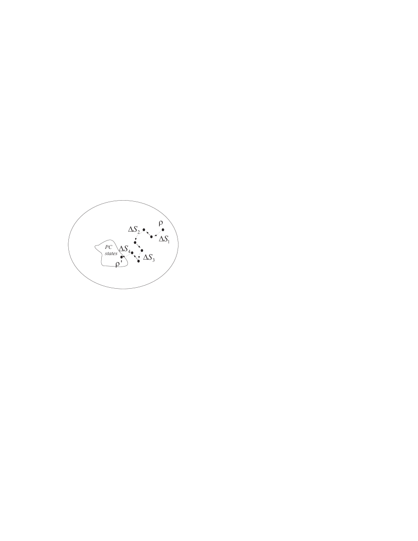
Figure 1: CLOCC protocol of concentration of information to local form is a series of actions aiming to reach the set of pseudo-classically correlated states. The continuous lines denote reversible actions: sending dephased qubits or local unitary transformations. The dotted lines denote dephasings. The goal is to make the total entropy increase $\Delta S=\Delta S_{1}+\Delta S_{2}+\ldots$ minimal. Then the deficit is given by $\Delta=\Delta S$, because once the state is pseudo-classically correlated, its full information content can be localized.

V.3 Defining cost of erasing entanglement

The above formulation of the deficit allows one to generalize the idea of thermodynamical cost to other situations. Namely, instead of the set of pseudo-classically correlated states one can take any other set and ask the same question: how much entropy must be produced, while reaching this set by use of CLOCC. Thus our concept of localizing information allows to ascribe thermodynamical costs to other tasks than localizing information. With any chosen set we can associate a suitable deficit $\Delta_{Set}$. An important application of this concept is to take set of separable states. Then the associated deficit $\Delta_{sep}$ has interpretation of thermodynamical cost of erasing entanglement. As such it is a good candidate for an entanglement measure. In this paper we will show that it is bounded from below by relative entropy of entanglement. Since set of separable states is a superset of pseudo-classically correlated states, we have

$$\Delta_{sep}\leq\Delta$$ (21)

so that the cost of erasing all quantum correlations is no smaller than cost of erasing entanglement. For sake of further proofs, let us put here formal definition of $\Delta_{sep}$

Definition 6.

The thermodynamical cost of erasing entanglement $\Delta_{sep}$ is given by

$$\Delta_{sep}(\rho)=\inf_{\cal P}(S(\rho^{\prime})-S(\rho)$$ (22)

where infimum runs over all CLOCC protocols ${\cal P}$ which transform initial state $\rho$ into separable output state $\rho^{\prime}$

VI Relations between deficit and relative entropy distance

In this section we will present the proof of the theorem relating deficit to in terms of relative entropy distance obtained in Horodecki et al. (2003a).

Theorem 1.

The information deficit is bounded from above by the relative entropy distance from the set of pseudo-classically correlated states.

$$\Delta(\varrho_{AB})\leq\inf_{\sigma\in{\cal P}{\cal C}}S(\varrho_{AB}|\sigma)\equiv E^{{\cal P}{\cal C}}_{r}$$ (23)

where $S(\varrho|\sigma)={\rm tr}\varrho\log\varrho-{\rm tr}\varrho\log\sigma$.

Let us first prove the proposition

Proposition 2.

Localisable information and deficit satisfies the following bounds:

$$I_{l}(\varrho)\geq N-\inf_{{\cal B}\in IPB}H(\varrho,{\cal B})$$ (24)

$$\Delta(\varrho)\leq\inf_{{\cal B}\in IPB}H(\varrho,{\cal B})-S(\varrho)$$ (25)

where $H(\rho,{\cal B})$ denotes the entropy of diagonal entries of state $\rho$ in basis ${\cal B}$

$$H(\rho,{\cal B})=-\sum_{i}p_{i}\log p_{i},$$ (26)

with $p_{i}=\langle\psi_{i}|\rho|\psi_{i}\rangle$, with $\psi_{i}\in{\cal B}$.

Proof. We will exhibit a simple protocol to achieve a reasonable amount of local information. Namely, Alice and Bob choose some implementable basis ${\cal B}$ and dephase a state in such basis. They can do this, as by definition, an IPB is a basis in which Alice and Bob can dephase by use of CLOCC. The final state has entropy

$$S(\rho^{\prime})=H(\rho,{\cal B}),$$ (27)

Alice and Bob can now choose the basis, that will produce the smallest possible entropy $H(\rho,{\cal B})$. In this way we obtain the following bound for $\Delta$:

$$\Delta\leq\inf_{{\cal B}\in IPB}H(\rho,{\cal B})-S(\rho)$$ (28)

This ends the proof of proposition.  

Let us now express this bound in terms of relative entropy distance. This is done by the following lemma.

Lemma 1.

Given a state $\varrho$,

$$H(\varrho,{\cal B})=\inf_{\sigma\in{\cal S}_{\cal B}}S(\varrho|\sigma)+S(\varrho),$$ (29)

where $H(\varrho,{{\cal B}})$ is the Shannon entropy of the probability distribution of the outcomes when $\varrho$ is measured in a given basis ${\cal B}$ and ${\cal S}_{\cal B}$ is the set of all states with eigenbasis ${\cal B}$.

Proof. We have

$$\inf_{\sigma\in{\cal S}_{\cal B}}S(\varrho|\sigma)+S(\varrho)$$

$$= \inf_{\sigma\in{\cal S}_{\cal B}}(-{\rm tr}(\varrho\log_{2}\sigma))$$

$$= -{\rm tr}(\varrho_{\cal B}\log_{2}\varrho_{\cal B})+{\rm tr}(\varrho_{\cal B}\log_{2}\varrho_{\cal B})$$

$$+\inf_{\sigma\in{\cal S}_{\cal B}}(-{\rm tr}(\varrho_{\cal B}\log_{2}\sigma))$$

$$= S(\varrho_{\cal B})+\inf_{\sigma\in{\cal S}_{\cal B}}S(\varrho_{\cal B}|\sigma)$$

$$= H(\varrho,{\cal B}).$$

Here $\varrho_{\cal B}$ is the state $\varrho$ dephased in the basis ${\cal B}$. In the second equality, we have used the fact that ${\rm tr}(\varrho\log_{2}\sigma)={\rm tr}(\varrho_{\cal B}\log_{2}\sigma)$, because $\sigma$ is diagonal in basis ${\cal B}$. In the fourth equality, we have used that $\varrho_{\cal B}$ belongs to the set ${\cal S}_{\cal B}$ so that $\inf_{\sigma\in{\cal S}_{\cal B}}S(\varrho_{\cal B}|\sigma)=0$, and also that $S(\varrho_{\cal B})\equiv H(\varrho,{\cal B})$. This ends the proof of the lemma.  

Now combining the lemma with the proposition we obtain the above theorem. We have not been able to prove equality, and in subsection VI.3 we discuss the origin of the difficulties.

VI.1 Deficit, cost or erasure of entanglement and relative entropy of entanglement

In the previous section we have reproduced the result of Horodecki et al. (2003a) which provided upper bound for deficit in terms of relative entropy distance from pseudo-classically correlated states. In this section we will prove a new result, providing a lower bound for the deficit in terms of an entanglement measure - the relative entropy of entanglement.

Theorem 2.

For any bipartite state $\rho$ the quantum deficit is bounded from below by relative entropy of entanglement

$$\Delta(\rho)\geq E_{r}(\rho)$$ (31)

To prove the above theorem it is enough to show that $\Delta_{sep}$ - the cost of erasing entanglement - is lower bounded by $E_{r}$, which is the contents of the next theorem. Indeed, by definition of $\Delta_{sep}$ and by the proposition 1 the deficit is no smaller than $\Delta_{sep}$.

Theorem 3.

For any bipartite state $\rho$ the quantum deficit is bounded from below by relative entropy of entanglement

$$\Delta_{sep}(\rho)\geq E_{r}(\rho)$$ (32)

To prove this theorem we will need the following lemma.

Lemma 2.

Consider any subset $S$ of states, invariant under product unitary transformations. Then relative entropy distance from this set $E_{r}^{S}$ given by

$$E_{r}^{S}=\inf_{\sigma\in{\cal S}}S(\rho|\sigma)$$ (33)

decreases no more than entropy increases under local dephasing, that is

$$E_{r}^{S}(\rho)-E_{r}^{S}(\Lambda(\rho))\leq S(\Lambda(\rho))-S(\rho)$$ (34)

where $\Lambda$ is local dephasing.

Proof. Note first that local dephasing can be represented as mixture of local unitaries:

$$\Lambda(\rho)=\sum_{i}p_{i}U^{i}_{A}\otimes I_{B}\,\rho\,{U_{A}^{i}}^{\dagger}\otimes I_{B}$$ (35)

Indeed, consider any set of projectors $\{P_{j}\}_{1}^{k}$. The suitable unitaries are given by

$$U(s_{1},\ldots,s_{k})=\sum_{j=1}^{k}s_{j}P_{j}$$ (36)

where $s_{j}=\pm 1$ are chosen at random. Thus $p_{i}$’s are equal, but this is irrelevant for our purpose.

Now, let us rewrite the inequality (34) as follows:

$$E_{r}^{S}(\rho)+S(\rho)\leq S(\Lambda(\rho))+E_{r}^{S}(\Lambda(\rho))$$ (37)

Thus we have to prove that function $f(\rho)=E_{r}^{S}(\rho)+S(\rho)$ is nondecreasing under dephasing. This is somehow parallel result to the result of Linden et al. (1999) where it was proven that the above function does not decrease under (global) mixing. The proof is directly inspired by Horodecki et al. (2004b).

We have

$$f(\Lambda(\rho))=\inf_{\sigma\in S}-{\rm tr}\Lambda(\rho)\log\sigma=$$ (38)

$$=\inf_{\sigma\in S}\sum_{i}p_{i}{\rm tr}\rho_{i}\log\sigma\geq\sum_{i}p_{i}\inf_{\sigma\in S}{\rm tr}\rho_{i}\log\sigma=$$

$$=\sum_{i}p_{i}\inf_{\sigma\in S}{\rm tr}\rho\log\sigma_{i}=\sum_{i}p_{i}\inf_{\sigma\in S}{\rm tr}\rho\log\sigma$$

$$=f(\rho)$$

where $\rho_{i}=U_{A}^{i}\otimes I_{B}\rho{U_{A}^{i}}^{\dagger}\otimes I_{B}$ and $\sigma_{i}={U_{A}^{i}}^{\dagger}\otimes I_{B}\sigma U_{A}^{i}\otimes I_{B}$. The inequality comes from properties of infimum, the last but one equality comes from the fact that the set $S$ is invariant under product unitary operations. This ends the proof of the lemma.  

Proof of the theorem 3. The basic ingredient of the proof is monotonicity of the function $f(\rho)=E_{r}(\rho)+S(\rho)$ under CLOCC. (In entanglement theory important functions are the ones that cannot increase under suitable class of operations, while here we need a function that does not decrease under our class of operations. This once more shows that our approach is in a sense dual to the usual entanglement theory.) As we have already discussed, any CLOCC operation can be decomposed into basic ones: (i) local unitary transformation, (ii) local dephasing and (iii) noiseless sending of dephased qubits. Of course local unitary operation does not change either entropy or $E_{r}$, so that the function $f$ remains constant. The lemma we have just proved tells us that local dephasing can only increase the function $f$. Consider now the last component - sending dephased qubits. Clearly entropy again does not change during such operations. It remains to show that $E_{r}$ does not change under sending dephased qubits. Consider the state $\rho_{ABB^{\prime}}$ with one dephased qubit $B^{\prime}$ on Bob’s site. Consider the closest separable state to the state $\sigma_{ABB^{\prime}}$. Since relative entropy of entanglement is in particular monotone under dephasings, we can choose this state to have the qubit $B^{\prime}$ dephased too. Consider then state $\rho_{AA^{\prime}B}$, where $A^{\prime}$ qubit is the $B^{\prime}$ qubit after being sent by Bob. We now apply the procedure of sending qubit $B^{\prime}$ to the state $\sigma_{ABB^{\prime}}$ and obtain a new separable state $\sigma_{AA^{\prime}B}$. By construction we have $S(\rho_{ABB^{\prime}}|\sigma_{ABB^{\prime}})=S(\rho_{AA^{\prime}B}|\sigma_{AA^{\prime}B})$. Thus $E_{r}$ could only go down. However we can repeat the reasoning with the qubit sent in converse direction, and conclude that $E_{r}$ does not change.

In this way we have shown that the function $f$ cannot decrease under CLOCC operations. This means, that for any protocol that brings initial state $\rho$ to a final separable state $\rho^{\prime}$ we have

$$f(\rho^{\prime})\geq f(\rho)$$ (39)

However the target state is separable, hence it has $E_{r}=0$. We obtain

$$S(\rho^{\prime})-S(\rho)\geq E_{r}(\rho)$$ (40)

which tells us that in any protocol that ends up with separable state, the increase of entropy is no smaller than relative entropy of entanglement. This ends the proof.  

VI.2 Connection with bounds obtained via semidefinite programming

In Synak et al. semidefinite programming techniques were used to obtain lower bounds on regularized deficit. The following general bound was obtained:

$$\Delta^{\infty}(\rho)\geq\sup_{\sigma}\left(-\log_{2}\lambda_{\max}(|\sigma^{\Gamma}|)-S(\varrho)-S(\varrho|\sigma)\right)$$ (41)

where $\lambda_{\max}$ denotes the greatest eigenvalue, and $\Gamma$ is partial transposition of the matrix. The value of the bound has been calculated for Werner states and isotropic states. It turned out that for those states it is exactly equal to regularized relative entropy of entanglement. This is compatible with the theorem 3. It is interesting, what is general relation of the bound (41) with regularized $E_{r}$.

VI.3 Discussion of the problem of ”noncommuting choice”

We have proved that deficit satisfies the following inequality

$$E^{{\cal P}{\cal C}}_{r}\geq\Delta\geq E_{r}$$ (42)

Yet we have not been able to prove that $\Delta=E^{{\cal P}{\cal C}}_{r}$. Let us discuss the main obstacles which we encountered. The question is actually as follows: Can there be better protocol than dephasing in optimal IPB basis? The latter protocol has some fundamental feature. Namely, in the series of the subsequent local dephasings, each dephasing is compatible with the previous one in the sense that they commute with each other. In other words, each dephasing is in some sense ultimate: it divides the total Hilbert space into blocks, so that all subsequent dephasings are performed within blocks, in the basis that is compatible with the blocks. Another way of viewing it is to say that what was sent from Alice to Bob or vice versa, will remain classical, that is diagonal in fixed distinguished basis. The main open question is now the following: Is it enough for Alice and Bob to follow this restriction, or whether they should violate this rule to draw more information?

We can formulate this fundamental problem in a more tractable way, if we look through the proof of the theorem 3, and find where the proof fails if instead of separable states one takes pseudo-classically correlated states. Almost the entire proof can be carried forward without alteration, apart from one small item: the invariance of $E^{{\cal P}{\cal C}}_{r}$ under sending dephased qubits. $E_{r}$ was invariant mainly because we could choose the closest separable state to be also dephased on that qubit. This is because set of separable states is closed under local dephasings. However the set of pseudo-classically correlated states is not. It does not rule out the possibility that indeed the closest pseudo-classically correlated state has the qubit dephased. However we were not able to prove it or disprove. We will formulate here the problem in a formal way:

Problem. Consider bipartite state that can be written in the following form:

$$\rho_{AB}=p_{1}\rho^{1}_{AB}+p_{2}\rho^{2}_{AB}$$ (43)

where $\rho^{1}_{AB}$ and $\rho^{2}_{AB}$ are orthogonal on subsystem $A$, i.e. the reduced states $\rho^{i}_{A}$ have disjoint support. Can the closest pseudo-classically correlated state in relative entropy distance be written in this form?

VI.4 Deficit and relative entropy distance for one-way and zero-way scenarios

Finally let us note that needed results can be obtained easily for one-way and zero-way scenarios. The problem with two-way is that Alice and Bob could draw more information than they obtain by measuring in optimal IPB basis. The source of difficulty was that in many rounds protocol, Alice and Bob could make dephasings that would not commute with dephasings they made in previous step. In the case of one-way there is no such danger, as there is only one round. The zero-way situation is simplest. The only thing Alice and Bob can do is to dephase the subsystems in some bases, and the only problem is to find optimal bases (so that they will produce the smallest amount of entropy). The versions of lemma 1 in one-way and zero-way case can be proven in the same way. Thus in those cases the deficits are equal to relative entropy distance to the two sets of states - classically correlated states and one-way classically correlated states (19).

VI.5 Multipartite states

We can define set of pseudo-classically correlated states also in the case of multipartite states. Then one can formulate version of Theorem 1 in the latter case. Since the arguments we have used did not depend on number of parties, Theorem is then true also in multipartite case. Similarly theorems 2 and 3 hold in the multipartite case.

VII Basic implications of the theorem (informational nonlocality)

The theorems obtained in the previous section allow us to obtain the following results for both bipartite as well as multipartite states.

• $\Delta$ is bounded no smaller than distillable entanglement $E_{D}$.

  $$\Delta\geq E_{D}$$ (44)

  Indeed, the latter is bounded from above by relative entropy of entanglement Rains (2000).

• Moreover, Theorem 3 implies that quantum deficit is no smaller than coherent information:

  $$\Delta(\rho)\geq S(\rho_{X})-S(\rho)$$ (45)

  where $X=A,B,C...$. or

  $$I(\rho)\leq N-S(\rho_{X})$$ (46)

  This is because it was proven that in bipartite case Plenio et al. (2000), relative entropy of entanglement is bounded from below by coherent information $S_{X}-S$. For multipartite states, one gets it by noting that multipartite relative entropy of entanglement is no smaller than the one versus some bipartite cut. Then one applies the mentioned bipartite result.

• Any entangled state is informationally nonlocal, i.e. it has nonzero deficit.

  $$\Delta(\varrho_{entangled})>0$$ (47)

  This follows form the fact that when a state is entangled, then it has nonzero relative entropy of entanglement.

  Note however that there exist separable states which are informationally nonlocal

  $$\Delta(\varrho_{separable})>0,$$ (48)

  for some separable states. We will now discuss an example of such state and relate it to so called ”nonlocality without entanglement”.

• Theorem 3 allows for easy proof that for pure bi-partite states the deficit is equal to entanglement. Indeed, from the theorem we have that deficit is no greater than entanglement. On the other hand, a simple protocol of dephasing Alice’s part in eigenbasis of the state of her subsystem, and sending the stuff to Bob gives the amount of information $2\log d-S(\rho_{A})$. Thus deficit is also no greater than entropy of subsystem. However the latter is equal to relative entropy of entanglement (this is reflection of the fact that in asymptotic regime there is only one measure of entanglement for pure states). For multipartite pure states there does not exists unique entanglement measure. We have the following open question: For multipartite pure states, is the deficit equal to relative entropy of entanglement?

  $$E_{r}(\psi)\mathop{=}\limits^{?}\Delta(\psi)$$ (49)

  If so, deficit would be an entanglement measure for all pure states. And since deficit is an operational quantity, we would have operational interpretation for relative entropy of entanglement for pure states.

  Note here that in general the deficit is not monotone under LOCC, and even under CLOCC. In contrast, $I_{l}$ is monotone under CLOCC.

• From the above reasoning and theorem 3 it follows that thermodynamical cost of erasure of entanglement of pure states is equal to their entanglement. (c.f. Oppenheim et al. (2002); Horodecki et al. (2003a))

VII.1 Non-locality without entanglement and with distinguishability

One form of non-locality we are familiar with, is entanglement. Another form of non-locality was introduced in Bennett et al. (1999a): so-called non-locality without entanglement. There, it was shown that there are ensembles of states, which, although product, cannot be distinguished from each other under LOCC with certainty. Ensembles of product states can have a form of non-locality. Other ensembles were exhibited, which were distinguishable, but distinguishing was thermodynamically irreversible. This can be thought of of as non-locality without entanglement but with distinguishability. All those results were done for ensembles.

Here we report similar kinds of nonlocality for states. Namely, we will exhibit states which are separable, and which can be created out of ensembles of distinguishable states but which contain unlocalizable information such that $\Delta\neq 0$ (at least for single copies). In fact, one can find such states which have an eigenbasis where each eigenket is perfectly distinguishable.

An example is the state given by

$$\rho=\frac{1}{4}|00\rangle\langle 00|+\frac{1}{4}|11\rangle\langle 11|+\frac{1}{2}|\psi^{-}\rangle\langle\psi^{-}|\,\,\,\,.$$ (50)

It is a separable state, which can be seen either by construction, or because it has positive partial transpose which is a sufficient condition for dimension $2\otimes 2$. It’s eigenkets $|00\rangle,|11\rangle,|\psi^{-}\rangle$ are clearly perfectly distinguishable under LOCC, since Alice and Bob just need to measure in the computation basis and compare results to know which of the three basis state they have. Nonetheless, it clearly has non-localisable information. To localize all the information, one would need to dephase it in the basis $|00\rangle,|11\rangle,|\psi^{-}\rangle$, but this cannot be done under CLOCC, since one cannot dephase using a projector on $|\psi^{-}\rangle$. The proof follows from Theorem 2 - we know that the optimal protocol is for Alice to dephase her side in some basis, and then send the state to Bob. Indeed, for two qubits, all implementable product bases are one-way implementable, i.e. they are of the form $\{|i\rangle|\psi^{(i)}_{k}\rangle\}$ where $\{|\psi^{(i)}_{k}\rangle\}$ are bases themselves. Thus for the one copy case, which we consider here, the optimal protocol is one-way protocol. Since the state is symmetric, then it does not matter which way (from Alice to Bob or vice-versa).

A direct calculation shows that the optimal basis is $|0\pm 1\rangle$ at one of the sites. This yields $I_{l}=3/4\log 3-1$, while $I=1/2$ giving a value of $\Delta=.1887$. There are thus separable states which exhibit non-locality in that all the information cannot be localized even though all the basis elements of the state are perfectly distinguishable.

VIII Informational nonlocality of multipartite states

The approach considered here turns out to be quite valuable in the case of multipartite states. One of the reasons for this is that one can not only quantify the quantumness of correlations along various splittings, as is commonly done, but one can also look at the total amount of localizable information that a given state possesses if all parties cooperate. In other words, in addition to the various vector measures defined for a particular splitting of the state eg. $AB|CD$, one also has a scalar measure which is defined for the state as a whole. One can calculate $\Delta$ for various bipartite splitting by grouping parties together, or one can calculate $\Delta$ for the entire state. In fact, one can consider all possible groupings, such as $AB|CD|EF$ etc. This allows one to explore multipartite correlations in more detail, and also allows one to ascribe a single quantity to a particular state in order to rank various states in terms of their total quantum correlations.

By considering a family of states for a number of parties $N$, one can calculate the information deficit per party $\Delta(\rho_{N})/N$. and we find that it goes to zero for the generalized GHZ, and to infinity for the Aharonov state, as $N$ goes to infinity. Of the states we consider, we shall thus find that the Greenberger-Horne-Zeilinger (GHZ) state is the least informationally nonlocal, while the so-called Aharonov state is the most informationally nonlocal.

VIII.1 Schmidt decomposable states

The information deficit for the N party GHZ state

$$|\psi_{NGHZ}\rangle=|111...1\rangle+|222...2\rangle+\ldots+|NNN...N\rangle$$ (51)

where we depart slightly from convention by taking the dimension of each parties state to also scale like $N$. This state is thus more entangled than if one were to give each party a qubit, and we do so in order to fairly compare our results with other entangled states. The deficit for the GHZ was calculated in Oppenheim et al. (2002) where it was found to be $\Delta(\psi_{NGHZ})=\log N$. Essentially, once one party makes a measurement, all the other parties can learn which state they have without performing a measurement, thus $I_{l}=(N-1)\log N$, while the total state is of dimension $N^{N}$, hence $I=N\log N$. Therefore

$$\lim_{N\rightarrow\infty}\Delta(\psi_{NGHZ})/N=0$$ (52)

This is in keeping with the notion that the GHZ is rather fragile, since if only one of the qubits becomes dephased, the entire state becomes classical.

One can generalize this to any multipartite state which can be written in a Schmidt basis. I.e.

$$|\psi_{NS}\rangle=\sum_{i}c_{i}\prod_{n=1}^{N}|\phi_{Ni}\rangle$$ (53)

In that case, one finds $\Delta(\psi_{NS})=S(\rho_{A})$ where $\rho_{A}$ is any of the subsystem entropies (they are all equal). This follows directly from inequality (46) and it holds in the asymptotic regime of many copies.

VIII.2 An example of a non-Schmidt decomposable state: The W state in three qubits

A more complicated example is the “$W$ state” Dür et al. (2000)

$$|\psi_{W}\rangle_{ABC}=\frac{1}{\sqrt{3}}(|100\rangle+|010\rangle+|001\rangle)$$

and we ask the question of how much localizable information $I_{l}$ can be extracted under one-way CLOCC by using it as a shared state. Since each party only has one qubit, we can use Theorem 2 to calculate it. This is because if each party only holds a single qubit, the optimal protocol will only need one way communication, and will be equivalent to having one party measure, and then tell her results to the other parties who will than hold a pure state between them.

Let Alice measure her part of the state in basis $\{|e_{i}\rangle\}$ and send the result to Bob and Charlie. After the measurement

$$|\psi_{W}\rangle_{ABC}\longrightarrow\varrho_{ABC}=\sum_{i}p_{i}|e_{i}\rangle\langle e_{i}|\otimes\varrho_{BC}^{i}$$ (54)

Then Alice obtains the ensemble $\{p_{i},|e_{i}\rangle\}$. Bob and Charlie obtain ensemble $\{p_{i},\varrho^{i}_{BC}\}$. $\varrho^{i}_{BC}$ are of course pure states. Bob and Charlie know, which of the states $\{\varrho^{i}_{BC}\}$ they have, because they have obtained information about the result of the measurement by Alice. Therefore, the total amount of information, that can be extracted from $|\psi_{W}\rangle_{ABC}$ locally, by such a protocol, is given by

$$I(\varrho_{A})+p_{1}I_{l}(\varrho^{1}_{BC})+p_{2}I_{l}(\varrho^{2}_{BC})$$ (55)

where $\varrho_{A}=\sum_{i}p_{i}|e_{i}\rangle\langle e_{i}|$ so that

$$I(\varrho_{A})=1-H(\{p_{i}\})$$ (56)

and where (since $\varrho_{B}^{i}$ are pure)

$$I_{l}(\varrho^{i}_{BC})=2-S(\varrho_{B}^{i}),$$ (57)

with $\varrho_{B}^{i}$ being the reduced density matrix of $\varrho^{i}_{BC}$. So for an arbitrary von Neumann measurement, we have that for the $W$ state, $I_{l}$ is given by

$$I_{l}(\psi_{W}) = 3-H(\{p_{i}\})-\sum_{1}^{2}p_{i}S(\varrho_{B}^{i})$$

$$= 3-H(\frac{1+|x|^{2}}{3})$$

$$- \frac{1+|x|^{2}}{3}H({1\over 2}+\frac{\sqrt{-3|x|^{4}+2|x|^{2}+1}}{2+2|x|^{2}})$$

$$- \frac{2-|x|^{2}}{3}H({1\over 2}+\frac{\sqrt{4|x|^{2}-3|x|^{4}}}{4-2|x|^{2}}),$$

where the measurement is performed in the basis $\{|e_{i}\rangle\}$ given by

$$\begin{array}[]{rcl}|e_{1}\rangle&=&x|0\rangle+y|1\rangle\\ |e_{2}\rangle&=&y^{*}|0\rangle-x^{*}|1\rangle.\end{array}$$

One can check that for von Neumann measurements, the largest amount of local information extractable is $1.45026$. It is achieved for measurement in the basis $\{|e_{i}\rangle\}$, where either $x^{2}=1/3$ or $x=2/3$ (see Figure 2). Contrary to naive expectations, dephasing in the computational basis is the worst choice. Also the basis $|\pm\rangle$ $(x=1)$ is not optimal. It is interesting, that optimal bases are not incidental. Rather these are those bases for which probabilities of transition into $|0\rangle,|1\rangle$ states are the same as the probabilities of getting those states by Alice measuring $W$ state in basis $|0\rangle,|1\rangle$. In the regime of single copies, this protocol is optimal by Theorem 2, therefore for the $W$ state, $I_{l}=1.45026$. This is less than the amount of localisable information for the corresponding GHZ state $|\psi_{GHZ}\rangle={1\over\sqrt{2}}(|000\rangle+|111\rangle)$, thus we would argue that the W-state exhibits more non-local correlations.

VIII.3 The Aharonov state and quasi-unlocalisable information

We next consider the so called, Aharonov “diamond” state. it is essentially given by anti-symmetrizing N N-dimensional states. For three parties, the unnormalized state is

$$|\psi_{3A}\rangle=|012\rangle-|021\rangle+|120\rangle-|102\rangle+|201\rangle-|210\rangle$$ (58)

and in general it is

$$|\psi_{NA}\rangle=\frac{1}{\sqrt{N!}}\sum_{permutations}\epsilon^{a_{1}...a_{N}}|a_{1}...a_{N}\rangle$$ (59)

where $\epsilon^{a_{1}...a_{N}}$ is the permutation symbol (Levi-Civita density).

It has the property that if one party measures their state in any basis, and tells their result to the rest of the parties, they will then still hold another Aharonov state of dimension $N-1$. Since this is a pure state of dimension $N^{N}$, the total amount of information is $I=N\log{N}$. On the other hand, under the protocol where the parties take turns measuring, it is easy to see that after each measurement, the other parties will still be left with a locally maximally mixed state. Finally, however, there will be two parties left, and they will share a singlet, which can be converted into $1$ bit of localized information.

The amount of localisable information is therefore $I_{l}=1$ regardless of how large $N$ is. This is optimal by Theorem 2 for single copies. We thus have that $\Delta(\psi_{NA})/N=\log{N}-1/N$ which grows logarithmically to infinity with $N$. The amount of localisable information per dimension goes very fast to zero as $N^{-N}$. The Aharonov state can then be thought of as a form of unlocalizable information. One might wonder if one can make the localisable information strictly zero, as is the case for entanglement with bound entangled states. We will soon show that this is not the case.

VIII.4 General pure three qubit states

In subsection VIII.1, we considered the localisable information of Schmidt decomposable states. And in subsection VIII.2, we considered the W state, an example of a non-Schmidt decomposable state.

Let us here consider the general three qubit pure state, which can be written in the form Acin et al. (2000); Carteret et al. (2000)

$$\left|\psi\right\rangle_{ABC}=a\left|000\right\rangle+b\left|010\right\rangle+c\left|100\right\rangle+d\left|001\right\rangle+e\left|111\right\rangle,$$ (60)

where only $a$ need be complex, while the rest of the coefficients are real. Of course we have $|a|^{2}+b^{2}+c^{2}+d^{2}+e^{2}=1$.

We again can use Theorem 2 to obtain the amount of localisable information. let us suppose that Alice (A) measures in the basis

$$\begin{array}[]{rcl}|e_{1}\rangle&=&x|0\rangle+y|1\rangle\\ |e_{2}\rangle&=&y^{*}|0\rangle-x^{*}|1\rangle,\end{array}$$ (61)

and sends the measurement outcome to Bob (B) and Charlie (C).

Depending on the measurement outcome, Bob and Charlie share the state

$$|\psi_{e_{1}}\rangle=\frac{1}{\sqrt{p}}((x^{*}a+y^{*}c)|00\rangle+x^{*}d|01\rangle+x^{*}b|10\rangle+y^{*}e|11\rangle)$$

or

$$|\psi_{e_{2}}\rangle=\frac{1}{\sqrt{1-p}}((ya-xc)|00\rangle+yd|01\rangle+yb|10\rangle-xe|11\rangle)$$

corresponding to the outcome $|e_{1}\rangle$ or $|e_{2}\rangle$ at Alice, where

$$p=|(x^{*}a+y^{*}c)|^{2}+|x|^{2}d^{2}+|x|^{2}b^{2}+|y|^{2}e^{2}$$

is the probability that $|e_{1}\rangle$ is obtained by Alice.

For such a protocol, the localisable information amounts to

$$I_{l} = \sup_{x,y}\big{[}3-H(p)-pS({\rm tr}_{A}|\psi_{e_{1}}\rangle\langle\psi_{e_{1}}|)$$ (62)

$$-(1-p)S({\rm tr}_{A}|\psi_{e_{2}}\rangle\langle\psi_{e_{2}}|)\big{]}$$

where we maximize over $x$ and $y$ to obtain the highest localisable information. This is an optimal protocol, and thus we obtain $I_{l}$. Let us denote the quantity in square brackets as $I_{l}^{xy}$.

Let us find the value of the localisable information for the case of the $W$ state $\left|\psi_{W}\right\rangle$, using Eq. (62). Without loss of generality, we may write $x=r>0$ and $y=\exp(i\phi)\sqrt{1-r^{2}}$. We now plot, in Fig. 2, the expression $I_{l}^{xy}$ on the $(r,\phi)$-plane. The supremum can then be read off from the figure. This supremum will then correspond to the localisable information for the $W$ state. Interestingly, the supremum is attained on two parallel lines on the $(r,\phi)$-plane.

Figure 2: Plot of $I_{l}^{x}$ versus $x^{2}$ for measurement in basis (61) for W-state. The optimal basis for maximizing $I_{l}^{x}$ is for Alice to dephase (or measure) with $x^{2}=1/3$ or $2/3$. The basis $|\pm\rangle$ ($x^{2}=1/2$) is not optimal.

Let us now choose an exemplary one-parameter subclass from the class in Eq. (60):

$$a=e=0,\quad b=0.1.$$

For this class, we plot the localisable information $I_{l}$ using real values of $x$ and $y$. Taking $x=r>0$ and $y=\sqrt{1-r^{2}}$, $I^{xy}_{l}$ is plotted (in Fig. 3) as a function of $r$ and $c$. For a given $c$ (which then fixes the state), the value of $I_{l}$ can be read from the figure.

Figure 3: Plot of the function $I_{l}^{xy}$ (Eq. (62) for the three-qubit state in Eq. (60) for the case when $a=e=0$, $b=0.1$, on the $(c,r)$-plane. Here $x=r$, $y=\sqrt{1-r^{2}}$, and $r>0$. The value of localisable information $I_{l}$ for a given $c$ is the supremum of $I_{l}^{xy}$ for that value of $c$.

IX Bell mixtures

The state of eq. (50) is a particular example of a mixture of Bell states

$$\begin{array}[]{rcl}\displaystyle\left|\phi^{\pm}\right\rangle&=&{\frac{1}{\sqrt{2}}\left(\left|00\right\rangle\pm\left|11\right\rangle\right)},\\ \left|\psi^{\pm}\right\rangle&=&{\frac{1}{\sqrt{2}}\left(\left|01\right\rangle\pm\left|10\right\rangle\right).}\end{array}$$

Here, for completeness, we calculate $\Delta$ for all states of this for - so-called Bell-diagonal states. Up to local unitaries, this includes all $2\otimes 2$ states with local density matrices that are maximally mixed. Due to Theorem 2, we only need consider optimizing over projection measurements (without adding any ancilla locally) at one of the parties, say Alice. Consider therefore the mixture

$$\varrho_{Bm}=p_{1}P_{\phi^{+}}+p_{2}P_{\phi^{-}}+p_{3}P_{\psi^{+}}+p_{4}P_{\psi^{-}}$$ (63)

of the four Bell states in $2\otimes 2$.

After an arbitrary projection valued (PV) measurement on Alice’s side, projecting in the basis

$$\left\{\left|\overline{0}\right\rangle=a\left|0\right\rangle+b\left|1\right\rangle,\quad\left|\overline{1}\right\rangle=\overline{b}\left|0\right\rangle-\overline{a}\left|1\right\rangle\right\},$$

let the global state be projected respectively to

$$P_{\left|\overline{0}\right\rangle}\otimes\varrho_{0},\quad P_{\left|\overline{1}\right\rangle}\otimes\varrho_{1}.$$ (64)

At this stage, the whole state is essentially on Bob’s side. This is because we allow dephasing as one of our allowed operations. Consequently, the locally extractable information after this set of operations is the von Neumann entropy of

$$pP_{\left|\overline{0}\right\rangle}\otimes\varrho_{0}+(1-p)P_{\left|\overline{1}\right\rangle}\otimes\varrho_{1},$$

where $p$ is the probability of Alice obtaining the state $\left|\overline{0}\right\rangle$. The optimization yields the value

$$\Delta=1+H(p_{1}+p_{2})-S(\varrho_{Bm})$$ (65)

where $p_{1}$ and $p_{2}$ are the two highest coefficients of the Bell mixture $\varrho_{Bm}$.

If we consider only von Neumann measurements (without addition of ancilla) and if Alice and Bob are not allowed to make any communication before they perform their measurements, then the zero-way information deficit $\Delta^{\emptyset}$ for the Bell mixtures (63) is given by

$$1+H(p_{\max}),$$

where

$$p_{\max}=\frac{1}{2}(1+|\max\{t_{11},t_{22},t_{33}\}|)$$

with $t_{ii}={\rm tr}(\sigma_{i}\otimes\sigma_{i}\varrho_{Bm})$. Note however that in this case, we are unable to show whether one can do better by POVMs or whether more copies are useful.

Consider however the isotropic $d\otimes d$ state

$$\varrho_{iso}=\lambda\left|\phi_{max}\right\rangle+(1-\lambda)\frac{I}{d^{2}}$$ (66)

in $d\otimes d$, where $\phi_{max}$ is the maximally entangled state in $d\otimes d$ which is invariant under $U\otimes U^{*}$ for any unitary $U$. The one-way information deficit $\Delta^{\rightarrow}$ (as well as $\Delta^{\emptyset}$) is given by

$$\Delta^{\emptyset}=\Delta^{\to}=(\lambda+\frac{1-\lambda}{d})\log_{2}(1+\frac{1-\lambda}{d})$$ (67)

$$+(d-1)\frac{1-\lambda}{d}\log_{2}\frac{1-\lambda}{d}-\log_{2}d+S(\varrho_{iso})$$

where

$$S(\varrho_{iso})=-(\lambda+{1-\lambda\over d})\log(\lambda+{1-\lambda\over d})-$$ (68)

$$-{d^{2}-1\over d^{2}}(1-\lambda)\log{1-\lambda\over d^{2}}$$

For the isotropic state, it is possible to prove, on the same lines as for Bell mixtures, that POVMs as well as more than one copy cannot help.

IX.1 Asymptotic regime

For two qubits we easily evaluated deficit, because, one-way and two-way deficits are equal in this case, because Alice’s first measurement leaves no room for other measurements. So the only thing she should do is to communicate results to Bob, and communication from Bob is not needed. Put it in other words: set of pseudo-classically correlated states is equal to the one-way classically correlated states of the form (19). Thus it was enough to evaluate only one-way deficit. However if we turn to regularization, this equivalence is no longer valid. This is because, to calculate regularization, one needs to evaluate deficit for many copies. Thus the dimension of the system is high, and there is room for many rounds. we are not able to regularize two-way deficit.

Concerning one-way deficit, one can argue that it is additive for Bell diagonal states. Moreover, borrowing qubits that borrowing qubits does not help (It has been independently shown that in general, in one-way case, borrowing pure local qubits does not help Devetak ). We will provide the argumentation in section XIV.1.

X Purely unlocalisable information doesn’t exist

One important aspect of entanglement theory is the existence of bound entangled states. These are states which are entangled, in that they require entanglement to create, yet no entanglement can be drawn from them. In Section VIII.3 we saw that in the multipartite case, there were states which the amount of localisable information per party went to zero as the number of parties increased. One can ask whether there is a strict analogy to bound entanglement: are there states which have positive $I$, but which $I_{l}=0$. It turns out that the answer is no; the only state which has $I_{l}=0$ is the maximally mixed state. Here we prove this in the following lemma for the case of two parties. The generalization to many parties is straightforward.

Lemma 3.

¿From any state other than the maximally mixed state we can draw local information.

Proof.

Consider a state $\varrho\sim C^{d}\otimes C^{d}$ such that $\varrho\neq\varrho_{mmix}=\frac{I}{d^{2}}$, then there exists an observable for which the mean value in state $\varrho$ has a different value than $\varrho_{mmix}$. Every nonlocal observable can be decomposed into local operators, so we can always find such an observable of the form $A\otimes B$ for which:

$$Tr(A\otimes B)\varrho\neq Tr(A\otimes B)\frac{I}{d^{2}}$$ (69)

Then

$$Tr(A\otimes B)\varrho\neq\frac{1}{d^{2}}TrATrB$$ (70)

$$\sum_{ij}p_{ij}\lambda_{i}\lambda_{j}\neq\sum_{ij}\frac{1}{d^{2}}\lambda_{i}\lambda_{j}$$ (71)

Notice that distribution of probability for $\varrho$ in (71) is classical. We know that we can obtain a nonzero amount of local information from any classical state besides the maximally mixed one. We can see that we are able to find such local operation, that transforms every state which agrees with the assumptions of lemma 3, into a state from with we can draw local information. ∎

There is an open question, whether there exist states, for which localisable information is entirely equal to local information content, but which nevertheless are not product. In such case, one wouldn’t be able to draw information from correlations at all. The classical deficit $\Delta_{c}$ would be zero, even though state would be non-product. It is rather unlikely that such states exist, yet we have not been able to solve this question.

We now prove a related theorem which follows from the above lemma, and which will be useful for the following section. Namely, we show that using pure states as a resource cannot help when distilling local information. One can think of such a process as catalysis where one uses pure states to produce more pure states from some shared state.

Theorem 4.

Local pure ancillas do not help in process of distilling local information.

Proof. Assume that catalysis can help in drawing local information. Consider a state $\varrho$, which is not the maximally mixed state and the optimal protocol of distilling local information $P_{1}$, which do not use ancillas. Consider also another protocol $P_{2}$, in which we distill information from some of the copies of state $\varrho$. Using $P_{1}$ and then use the distilled pure states to do catalytic distillation on the rest of copies. Notice, that we can do this, because we know from lemma 3 that we can distill local information thus also pure states from it. If catalysis is helpful that means that using $P_{2}$ we are able to obtain more local information than in previous protocol. Protocol $P_{2}$ does not use ancillas and is better than $P_{1}$, which is optimal. This leads to the required contradiction.

We showed that catalysis is useless for state with nonzero distillable information. It could help only in cause of states with pure unlocalisable information, but we know from Lemma 3 that such states do not exist. This ends the proof.

Remark. We know that to do catalytic distillation we need pure ancillas. One can notice that states, which we want to use in protocol $P_{2}$ to do catalysis are not exactly pure. But these states come from distillation, so they are equal in the limit of many copies to $|0\rangle^{\otimes rn}$ ($r$ is rate of distillation of local information and $n$ is the amount of copies). This fact assure us that in asymptotic regime of many copies we are able to catalysis.

XI Can correlations be more quantum than classical?

The total amount of correlations contained in a bipartite state is given by the mutual information

$$I_{M}=S(\rho_{A})+S(\rho_{B})-S(\rho_{AB})$$ (72)

One can easily see that our quantities for dividing correlations into ones which behave quantumly ($\Delta$) and classically ($\Delta_{c}$) satisfy

$$I_{M}=\Delta+\Delta_{c}\,\,\,\,.$$ (73)

In other words, the total amount of correlations (given by $I_{M}$) can be divided into classical and quantum components. Now one can ask whether the total correlations $I_{M}$ can be divided arbitrarily. Certainly for pure states, this is not the case. For pure states, correlations which behave quantumly cannot exceed $I/2$. For pure states $\psi$, we showed that $\Delta=S(\rho_{A})$, and thus it is always the case that $\Delta(\psi)=I_{M}/2$. For pure states, the quantumness of correlations can never exceed the classicalness of correlations.

Now one can ask: Can it be that one has states for which

$$\Delta(\varrho_{AB})>I/2?$$ (74)

If so, one could think of these states as having super-saturated quantum correlations, in that for a given amount of mutual information $I_{M}$ they have a greater proportion of correlations which behave quantumly. In this sense, one can think of such states as being more non-local than maximally entangled states.

One way of approach to the above problem is to work with relative entropy of entanglement. We know that both the relative entropy of entanglement ($E_{r}$), with distance taken from separable states, and the von Neumann entropy ($S_{AB}$) are not greater than $\log_{2}d$ for $d\otimes d$ states. Consequently, one has $E_{r}+S_{AB}\leq 2\log_{2}d$. Can we have the following stronger inequality:

$$2E_{r}+S_{AB}\mathop{\leq}\limits^{?}2\log_{2}d.$$ (75)

This is tight for maximally entangled states. Because deficit is no smaller than relative entropy of entanglement, it follows that if the inequality is violated, then for some states inequality (74) is true, and we would have the curious phenomenon. On the other side, when the inequality is satisfied for all states, we would obtain a nice trade-off between entanglement and noise.

In a recent work, Wei et al. Wei et al. (2003) calculated (for two-qubit states) the maximal possible relative entropy of entanglement $E_{r}$ (as well as other entanglement measures) for a given amount of mixedness (quantified by the von Neumann entropy). Note that the inequality (75) would generically hold for two-qubit states if it is satisfied by these optimal values. Indeed examining the curves of the above paper, one finds that for any two qubit state the inequality is satisfied.

One can also find that for Werner states, and maximally correlated states, the inequality is satisfied too, for regularized relative entropy of entanglement. To see this, the asymptotic relative entropy of entanglement ($E_{r(PPT)}^{\infty}$) (with distance taken from states with positive partial transpose (PPT)) is known for Werner states (mixture of projectors on symmetric and antisymmetric spaces) in $d\otimes d$ Audenaert et al. (2001). One may check that the relation

$$2E_{R(PPT)}^{\infty}+S_{AB}\leq 2\log_{2}d$$ (76)

is satisfied for all Werner states in arbitrary dimensions. However, note here that the relative entropy of entanglement (from PPT states) is not additive for Werner states.

For the maximally correlated states, relative entropy of entanglement (from PPT states) is known to be additive. Its value is also explicitly known for all such states in $d\otimes d$. Via additivity, this would exactly be equal to its asymptotic relative entropy of entanglement (from PPT states). Precisely, for any state of the form

$$\varrho_{mc}=\sum_{ij}a_{ij}\left|ii\right\rangle\left\langle jj\right|,$$

we have

$$E_{R(PPT)}^{\infty}=E_{R(PPT)}=\sum_{i}a_{ii}\log_{2}a_{ii}-S(\varrho_{mc}).$$

It is easy to check that the relation (76) is satisfied by any $\varrho_{mc}$ in $d\otimes d$.

Thus we haven’t found states for which the inequality would be violated for regularized relative entropy of entanglement. It remains an open question whether the trade-off between noise and entanglement represented by inequality is universally true, or whether there exist states, for which there is more quantum than classical correlations.

XII Zero-way and one-way subclasses

We now turn to additional measures of quantumness of correlations which arise when one restricts the communications between Alice and Bob. In sections IX, VIII such restrictions were useful for evaluations of perhaps more basic two-way quantities. However they are more than just for ease of calculation - we shall also see that the restricted measures allow one to explore other aspects of non-locality. Additionally, there appears to be strong connections between the deficit and distillation of randomness from shared states. For example, it has just been shown in Devetak that the one-way deficit is equal to the mutual information minus the one-way distillable randomness Devetak and Winter .

As before, the optimal protocols by which the corresponding local informations are obtained amounts to producing “classical-like” states of least entropy by the respective operations. As mentioned in section V.2 the theorems proven there apply equally well in these restricted scenarios with suitable modification.

In any protocol of concentrating information to local form, the parties can stop at states of the form

$$\varrho_{AB}^{\prime}=\sum_{ij}p_{ij}\left|i\right\rangle\left\langle i\right|\otimes\left|j\right\rangle\left\langle j\right|.$$ (77)

However for two-way scenario, we have argued that one can stop already at pseudo-classically correlated states. When one-way protocols are allowed, it is sufficient for the parties to stop at states of the form

$$\varrho_{AB}^{\prime}=\sum_{i}p_{i}\left|i\right\rangle\left\langle i\right|\otimes\varrho_{i}.$$ (78)

Finally for zero-way protocols, one has to achieve classical states (77). Consider for example the zero-way protocol for a state $\varrho_{AB}$ by which $I_{l}^{\emptyset}$ is attained. Without any classical communication (just by dephasing via an environment), Alice and Bob change the state $\varrho_{AB}$ into a classical-like state $\varrho^{\prime}_{AB}$ (of the form given in eq. (77)), so that $S(\varrho^{\prime}_{A})+S(\varrho^{\prime}_{B})$ is minimized, where $\varrho^{\prime}_{A}$ and $\varrho^{\prime}_{B}$ are the local density matrices of $\varrho^{\prime}_{AB}$. Note that the parties must concentrate information using classical communication. But this is only after they have performed all their dephasings. The situation is therefore like in a Bell-type experiment.

Let us now show that $\Delta^{\emptyset}$ is an independently useful candidate for quantum correlations and can capture interesting aspects of non-locality. The states that contain no quantum correlations would be then the ones with $\Delta^{\emptyset}=0$. Consider for example the states with eigenbasis (without normalization)

$$\left|0\right\rangle_{A}\left|0\right\rangle_{B},\left|0\right\rangle_{A}\left|1\right\rangle_{B},\left|1\right\rangle_{A}(\left|0\right\rangle+\left|1\right\rangle)_{B},\left|1\right\rangle_{A}(\left|0\right\rangle-\left|1\right\rangle)_{B},$$ (79)

where $\left|0\right\rangle$ and $\left|1\right\rangle$ are the eigenvectors of the Pauli matrix $\sigma_{z}$. Such states are the ones used in the BB84 quantum cryptography protocol Bennett and Brassard (1984). This set of orthogonal states are distinguishable locally. But they are not distinguishable by zero-way communication. Bob must wait for Alice’s measurement result (in the $\sigma_{z}$-basis) to decide whether to perform a measurement in the $\sigma_{z}$-basis or in the $\sigma_{x}$-basis. Therefore a mixture of the states in eq. (79), where the mixing probabilities are all different from each other (so that the spectrum of the resulting state is non-degenerate), would have nonvanishing $\Delta^{\emptyset}$. This is because an arbitrary dephasing by Bob on such a mixture, before obtaining Alice’s result would result in no information being extracted from the state (by Bob). Consequently there would be an information deficit when trying to extract information locally, because globally of course all the information is extractable from such a state. All the information is also extractable by one-way or two-way communication. This is contrast to states which have an eigenbasis

$$\left|0\right\rangle_{A}\left|0\right\rangle_{B},\left|0\right\rangle_{A}\left|1\right\rangle_{B},\left|1\right\rangle_{A}\left|0\right\rangle_{B},\left|1\right\rangle_{A}\left|1\right\rangle_{B},$$

for which all the information is extractable from the state locally, by measurement by both the parties in the $\sigma_{z}$-basis, without any communication.

We therefore see that the quantum behavior of correlations could result from the distinctly quantum but “local” property of nonorthogonality. Here we call nonorthogonality a local property, as it does not a priori require a tensor product structure to manifest itself. It is this nonorthogonality that manifests itself in a more complex form in the examples of LOCC-indistinguishable orthogonal product bases Bennett et al. (1999a, b); DiVincenzo et al. . More generally, it may be the reason for any case of LOCC-indistinguishability of orthogonal states Walgate and Hardy (2002); Ghosh et al. (2001, 2002); Horodecki et al. (2003c); Chen and Li (2003).

An interesting issue is relation between $\Delta^{\emptyset}$ and mutual information. In section XI we have asked a question whether there exist states for which $\Delta$ would be more than half of mutual information. The same question can be asked in the case of one-way and zero-way deficits. Łukasz Pankowski has performed numerical simulations to evaluate $\Delta^{\emptyset}$ versus mutual information. The results are presented on figure 4. Surprisingly, there are states, for which the deficit is almost equal to mutual information. Thus the measurement destroys almost all correlations! The quantum correlations do not imply classical correlations (see DiVincenzo et al. (2004) in this context).

Figure 4: Zero-way deficit is plotted versus mutual information for 100 000 random two qubit states. The upper line stands for $\Delta^{\emptyset}=I_{M}$. The lower line denotes isotropic states of eq. (66). Two regimes are evident: in first regime, there are states, for which deficit is almost equal to mutual information.

With respect to the pure states considered in Section IV.6, it is easy to see that $\Delta$ is also equal to $\Delta^{\rightarrow}$. This is also true for single copies of single qubit states, due to Theorem 2.

XII.1 Expression for one-way $\Delta$

In this subsection we consider the expression for the one-way deficit In the case when only one-way communication is allowed between the parties, the only thing that Alice and Bob can do, is that Alice dephases her part in come basis, and then sends her part to Bob. Dephasing transforms the state as

$$\varrho_{AB}\to\varrho^{\prime}_{AB}=\sum_{i}P_{i}\otimes I\varrho_{AB}P_{i}\otimes I=\sum_{i}p_{i}\left|i\right\rangle\left\langle i\right|\otimes\varrho_{B}^{i}$$

where $\left\{P_{i}=\left|i\right\rangle\left\langle i\right|\right\}$ forms a set of orthogonal one-dimensional projectors on the Hilbert space of Alice’s part of $\varrho_{AB}$ and $p_{i}$ are probabilities of the corresponding outcomes which Alice would obtain if she performed measurements with the same $P_{i}$’s rather than dephasing, while $\varrho_{B}^{i}$ is the state that Bob would obtain conditionally on measurement outcome $\left|i\right\rangle$. Thus

$$p_{i}={\rm tr}(\varrho_{AB}P_{i}\otimes I)$$ (80)

$$\varrho_{B}^{i}={1\over p_{i}}{\rm tr}_{A}(P_{i}\otimes I\varrho_{AB}P_{i}\otimes I)$$

The process of sending does not change the form of the state, so that the entropy of the final state at Bob is

$$S(\varrho^{\prime}_{AB})=S(\varrho_{A}^{\prime})+\sum_{i}p_{i}S(\varrho_{B}^{i})$$

where $\varrho_{A}^{\prime}=\sum_{i}p_{i}\left|i\right\rangle\left\langle i\right|$ is the reduced density matrix of the $A$-part of $\varrho^{\prime}_{AB}$. So finally $I_{l}^{\to}$ takes the form

$$I_{l}^{\to}=n_{AB}-\inf_{\{P_{i}\}}(S(\varrho_{A}^{\prime})+\sum_{i}p_{i}S(\varrho_{B}^{i}))$$

and correspondingly

$$\Delta_{l}^{\to}=\inf_{\{P_{i}\}}(S(\varrho_{A}^{\prime})+\sum_{i}p_{i}S(\varrho_{B}^{i}))-S(\varrho_{AB}).$$ (81)

Just as we showed that $\Delta$ was equal to the relative entropy distance to pseudo-classically correlated states, one can also write $\Delta^{\rightarrow}$ and $\Delta^{\emptyset}$ as the minimum relative entropy distance to the set of states $\cal{S}^{\rightarrow}$ and $\cal{S}^{\emptyset}$ which can be created reversibly under the one-way and zero way classes of operations.

XIII Relationship with other measures of quantumness of correlations

Let us now compare the deficit with other measures of quantumness of correlations, in particular the quantum discord Zurek (2000); Ollivier and Zurek (2002). The latter is defined formally, as the difference of two classically equivalent expressions for the mutual information, applied to quantum systems (taken to be a measuring apparatus and system). It was defined with respect to a measurement $A_{\cal M}$ (either a projective one, or a POVM (Positive Operator Valued Measure) performed on the apparatus A. One then defines the discord $\delta(A_{{\cal M}}|B)$ with respect to this measurement that results with probabilities $p_{i}$ in joint states $\varrho_{AB}^{\prime i}=(|\psi_{i}\rangle\langle\psi_{i}|)^{A}\otimes\varrho_{i}^{B}$. The discord is defined as

$$\delta(A_{{\cal M}}|B)=H(\{p_{i}\})+\sum_{i}p_{i}S(\varrho_{i})-S(\varrho_{AB})\,\,\,\,.$$ (82)

The relationship between $\delta(A_{{\cal M}}|B)$ and $\Delta^{\rightarrow}$ (defined on single copies) was recently shown in Zurek (2003) where it was shown that the discord also has the interpretation of extraction of work by a demon, if one minimizes $\delta(A_{{\cal M}}|B)$ over all possible measurements $A_{{\cal M}}$. Care however must be taken, since with the definition of discord there is no cost associated to pure states which are used in a POVM. Therefore, we note here that the relationship between the discord and $\Delta^{\rightarrow}$ only applies if one optimizes the discord over von Neumann measurements, and disallows POVMs.

Finally, let us provide two explicit examples of cases where two way communication is more powerful than 1-way communication. I.e one has the strict inequality $\Delta^{\leftrightarrow}>\Delta^{\rightarrow}=\inf_{A_{{\cal M}}\in PVmeas}\delta(A_{{\cal M}}|B)$

To this aim consider the basis related to the sausage states of Bennett et al. (1999a) and which has been analyzed in Oppenheim et al. (2003a):

$$\begin{array}[]{lll}&{\mbox{\small}A}&{\mbox{\small}B}\\ \psi_{1}=&|0+1\rangle&|2\rangle\\ \psi_{2}=&|0-1\rangle&|2\rangle\\ \psi_{3}=&|0\rangle&|0+1\rangle\\ \psi_{4}=&|0\rangle&|0-1\rangle\\ \psi_{5}=&|1+2\rangle&|0\rangle\\ \psi_{6}=&|1-2\rangle&|0\rangle\\ \psi_{7}=&|1\rangle&|1\rangle\\ \psi_{8}=&|2\rangle&|2\rangle\\ \psi_{9}=&|2\rangle&|1\rangle\\ \end{array}$$ (83)

Consider now any bipartite $3\otimes 3$ state $\varrho_{two-way}$ that is diagonal in the above basis, but has nondegenerate spectrum. It is relatively easy to provide a two-way protocol that distinguishes vectors (83) without destroying them (see Oppenheim et al. (2003a)). Hence $\Delta^{\leftrightarrow}$ vanishes. Evidently $\varrho_{two-way}$ is not of the form $\sum_{i=1}^{3}|\phi_{i}\rangle\langle\phi_{i}|\otimes\varrho_{i}$ with orthogonal $\phi_{i}$, since there are no three eigenvectors among (83) that have the same component on Alice’s side. So both $\Delta^{\rightarrow}$ and discord are strictly positive for this state. Thus Maxwell’s demon which communicate in both directions are more powerful than demon’s who can only communicate in one direction.

Another simple example is to take states which have zero optimized discord or one-way deficit

$$\rho_{\rightarrow}=\sum_{i}p_{i}|i\rangle_{A}\langle i|_{A}\otimes\rho^{i}_{B}\,\,\,\,\,\,\,\,,\rho_{\leftarrow}=\sum_{j}p_{j}\rho^{j}_{A}\otimes|j\rangle_{B}\langle j|_{B}$$ (84)

but in different directions of communication. Then take them each to be on orthogonal Hilbert spaces, and mix. Such a state will have $\Delta^{\leftrightarrow}=0$ since both parties can just project on the two orthogonal Hilbert spaces to determine whether they hold $\rho_{\rightarrow}$ or $\rho_{\leftarrow}$ and then the appropriate party can send her state down the channel. On the other hand, one-way communication will be sufficient to completely localize one of the states but not always both.

XIV Relation with measures of classical correlation

In this section we shall analyze the relation of the classical deficit Oppenheim et al. (2003a) to already known measures of classical correlations. It happens that both zero-way and one-way deficit have their ”counterparts” in such measures. There is no known analog, however, for two-way deficit.

Let us recall that just as the quantum deficit was defined as

$$\Delta=I-I_{l}$$

One can think of it as describing how much better Alice and Bob can do under closed operations (CO) if they are given a quantum channel instead of the classical channel. Because it feels the difference between the quantum and classical channel, it tells us about the quantumness of correlations. Likewise, the classical deficit is given by

$$\Delta_{c}=I_{l}-I_{LO}$$

It tells us how much better two parties can do at localizing information if, instead of having no access to a channel i.e. closed local operations, they have access to a classical channel. Because the added resource is a classical channel, it shows how much better the parties can do by exploiting a classical channel.

One can verify that $\Delta_{c}$ and $\Delta$ add up to the quantum mutual information $I_{M}(\varrho_{AB})=S(\varrho_{A})+S(\varrho_{A})-S(\varrho_{AB})$. Thus

$$\Delta_{cl}=I_{M}-\Delta$$

More explicitly we have (cf eq. (11))

$${\Delta_{cl}}(\varrho_{AB})=S(\varrho_{A})+S(\varrho_{B})-\inf_{CLOCC}(S(\varrho^{\prime}_{A})+S(\varrho^{\prime}_{B}))$$

i.e. ${\Delta_{cl}}$ is the optimal decrease of local entropies by means of CLOCC.

XIV.1 One-way measures

Corresponding to the measure of quantumness of correlation under one-way classical communication (from Alice to Bob) ($\Delta^{\rightarrow}$), given by eq. (81), we could have the following formula for classical correlation:

$$\begin{array}[]{rcl}&&{\Delta_{cl}}^{\to}(\varrho_{AB})\\ &=&\sup_{P_{i}}[\{S(\varrho_{A})-S(\varrho^{\prime}_{A})\}+\{S(\varrho_{B})-\sum_{i}p_{i}S(\varrho_{B}^{i})\}]\\ &\equiv&\sup_{P_{i}}[{\delta}S(A)+{\delta}S(B|A)].\end{array}$$ (85)

Note that the supremum is taken over all local dephasings on Alice’s side. Although we optimize over projection measurements, one can effectively include POVM’s by including all the required ancillas from the start. Remarkably, it has been shown Devetak that POVM’s need not be considered when one goes to to the limit of many copies.

In eq. (85), we have distinguished two terms. The second term

$${\delta}S(B|A)=S(\varrho_{B})-\sum_{i}p_{i}S(\varrho_{B}^{i})$$

shows the decrease of Bob’s entropy after Alice’s measurement. The first one

$${\delta}S(A)=S(\varrho_{A})-S(\varrho^{\prime}_{A})$$

denotes the cost of this process on Alice side, and is non-positive. It is zero only if Alice measures in the eigenbasis of her local density matrix $\varrho_{A}$.

The expression for ${\Delta_{cl}}^{\to}$ is very similar to the measure of classical correlation introduced by Henderson and Vedral Henderson and Vedral (2001):

$${C_{HV}}=\sup_{P_{i}}(S(\varrho_{B})-\sum_{i}p_{i}S(\varrho_{B}^{i})).$$ (86)

Originally the supremum was taken over POVMs, but as mentioned we take the state acting already on a suitably larger Hilbert space, unless stated otherwise explicitly.

The difference between the Henderson-Vedral classical correlation measure and one given in eq. (85) is that the former does not include Alice’s entropic cost ${\delta}S(A)$ of performing dephasing. Hence in general,

$$\Delta_{cl}^{\rightarrow}\leq\Delta_{HV}.$$

In the asymptotic limit of many copies, one has equality Devetak . Actually in Devetak it was shown that regularized one-way classical deficit is equal to another operational measures of classical correlations: distillable common randomness introduced in Devetak and Winter . The latter is in turn equal to regularized Henderson-Vedral measure. It is interesting that $\Delta_{cl}^{\rightarrow}$ without regularization, although seems to be an important characteristics of classical correlations, does not meet a basic requirement for being a measure of classical correlations: it is not monotonous under local operations Synak and Horodecki . Thus regularization plays here a role of monotonization. There is interesting question what happens with two-way classical deficit after regularization.

XIV.2 Additivity of one-way quantum and classical deficits for Bell diagonal states

Here we will prove the fact mentioned in section IX.1, that the one-way deficits are additive, and that borrowing pure qubits does not help for Bell diagonal states. First of all in Terhal et al. (2002) it was shown that a measure of classical correlations $C_{HV}$ is additive for Bell diagonal states. Let us recall the argument, as it will be useful for making connection with classical deficit. For a Bell diagonal state $\rho$, consider a related channel $\Lambda$ (i.e. such channel that $(I\otimes\Lambda)(|\phi\rangle^{+}\langle\phi^{+}|)=\varrho$). The maximum output Holevo function over all input ensembles, denoted by $\chi^{*}(\Lambda)$ is, for general channels, no smaller than $C_{HV}$. They are equal, if the density matrix of ensemble attaining $\chi^{*}$ is equal to $\varrho_{A}$. In the case of Bell diagonal states, we have $\varrho_{A}=I/2$, and it turns out that the optimal ensemble for corresponding channels consists of two orthogonal states, hence gives rise to the same matrix. King King has shown that $\chi^{*}$ is additive for channels coming from the Bell diagonal states. ¿From this and from the fact that, in general, $\chi^{*}\geq C_{HV}$ one gets that for Bell diagonal states $C_{HV}$ for many copies is also equal to $\chi^{*}$ for many copies of corresponding channels. This proves that $C_{HV}$ must be additive.

Now, let us make connection with classical deficit. As discussed in Synak and Horodecki , if $\chi^{*}$ is attained on such ensemble that its density matrix is equal to $\varrho_{A}$, then by looking at ensemble maximizing $\chi$, one can tell something about measurements that attain $C_{HV}$. Namely, when the ensemble is orthogonal, then one attains $C_{HV}$ by measurement in eigenbasis of $\varrho_{A}$. Now, it is obvious from eq. (85) and discussion thereafter, that in the latter case $C_{HV}$ is actually equal to classical deficit, as they differ from one another only by entropy production during Alice’s measurement, which vanishes, if it is done in eigenbasis. Since $C_{HV}$ is additive, then for many copies it is again attained by measurement in orthogonal basis that is eigenbasis of Alice’s subsystem. Thus classical deficit for many copies is also not less than $C_{HV}$, and it by eq. (85) cannot be greater.

Thus for Bell diagonal states the deficit is equal to $C_{HV}$ and it is additive. Moreover, since the measurement was von Neumann one, the deficit is attained without using POVMs. This means that additional pure ancillas do not help.

So far we have talked about classical deficit. Now, since quantum and classical deficit add up to mutual information which is additive, it follows that quantum deficit is additive too. Also, since borrowing local qubits does not increase classical deficit, it cannot decrease quantum deficit.

XIV.3 Zero-way measures

Let us now consider measures of classical correlations under no classical communication, ${\Delta_{cl}}^{\emptyset}$. Again, this is taken to mean that the parties are not allowed to communicate before making measurements, but can do so afterward in order to concentrate the classical records. The information deficit under no classical communication, $\Delta^{\emptyset}$, is given by

$$\Delta^{\emptyset}=S(\varrho_{AB})-S(\varrho^{\prime}_{AB})$$

where $S(\varrho^{\prime}_{AB})$ is the von Neumann entropy of the optimal final state $\varrho^{\prime}_{AB}$ (which is classical-like), and was obtained by local complete measurements, without classical communication. We then obtain

$$\begin{array}[]{rcl}&&{\Delta_{cl}}^{\emptyset}=S(\varrho_{A})+S(\varrho_{B})-S(\varrho^{\prime}_{AB})\\ &=&\{S(\varrho_{A})-S(\varrho^{\prime}_{A})\}+\{S(\varrho_{B})-S(\varrho^{\prime}_{B})\}\\ &&+\{S(\varrho^{\prime}_{A})+S(\varrho^{\prime}_{B})-S(\varrho^{\prime}_{AB})\}\\ &\equiv&{\delta}S(A)+{\delta}S(B)+I_{M}(\rho^{\prime})\end{array}$$

We have three terms here: the last one

$$I_{M}(\rho^{\prime})=S(\varrho^{\prime}_{A})+S(\varrho^{\prime}_{B})-S(\varrho^{\prime}_{AB})$$

is the classical mutual information of the final state, while the first two, ${\delta}S(A)=S(\varrho_{A})-S(\varrho^{\prime}_{A})$ and ${\delta}S(B)=S(\varrho_{B})-S(\varrho^{\prime}_{B})$, denote respectively the local entropic costs of the process at the respective sides. We therefore have a trade-off similar to that in the one-way case. And again there was defined a classical correlation measure Terhal et al. (2002) which consists only of the last term of our quantity

$$C^{\emptyset}=\sup_{P_{i}}I_{M}(\varrho^{\prime})$$ (87)

where $\varrho^{\prime}$ is obtained out of $\varrho$ by local complete measurements. Again the original definition of $C^{\emptyset}$ involved POVMs, but as we have suitably increased our Hilbert space from the very beginning, we need not do so.

XV Complementarity features of information in distributed quantum systems

Bohr was the first who recognized a fundamental feature of quantum formalism - complementarity between incompatible observables. Complementarity was not explicitly related to entanglement, now regarded as an important quantum information resource. Namely, Bohr’s complementarity concerned mutually exclusive quantum phenomena associated with a single system and observed under different experimental arrangements.

Let us comment on complementarity in the case of composite systems and Bohr complementarity. Roughly speaking, the latter says that one cannot access the properties of the systems necessary to describe it by one measurement. The rule is formulated for single quantum systems and is a consequence of noncommutativity.

On the other hand we know that one can also divide the properties of the system into local and nonlocal ones, and they are complementary with each other too Oppenheim et al. (2003a). For example, one can perform measurement in Bell basis or in standard product basis. However one cannot perform those measurements simultaneously. In other words one cannot access global and local properties of the system (see also Jak in this context).

The latter phenomenon is not merely a consequence of Bohr’s complementarity. Indeed, if the only allowable states of composite systems were the classically correlated states:

$$\rho=\sum_{ij}p_{ij}|e_{i}\rangle|f_{j}\rangle\langle e_{i}|\langle f_{j}|$$ (88)

then maximal information about the total system would be available through measurements on subsystems. Global measurements would not access any further knowledge about properties of the system. On the other hand, Bohr complementarity would still hold, in the sense that one cannot access all properties of the system in one measurement.

Thus we see that the local-nonlocal complementarity Oppenheim et al. (2003a) is a consequence of two distinct phenomena: noncommutativity and existence of entanglement (or quantum correlations). So not only is there noncommutativity, but there is too much of it, so that it affects also relations between local and nonlocal informational contents.

In distributed systems one usually imposes constraints by allowing operations that can be done solely by classical communication and local operations. It turns out that in such situation there also arises an interesting complementarity. Namely, in Oppenheim et al. (2003a) we considered two tasks: localizing information (which we have presented in this paper) and sending quantum information (e.g. teleportation), performed simultaneously. It was shown that for a fixed protocol ${\cal P}$, the rates of those two tasks obey the following relation

$$I_{l}({\cal P},\rho)+Q({\cal P},\rho)\leq I_{l}(\rho)$$ (89)

where $I_{l}({\cal P},\rho)$ is the amount of information localised by the protocol ${\cal P}$ and $Q({\cal P},\rho)$ is the amount of qubits transmitted by the protocol.

For example, for the singlet state, the total informational contents is equal to total correlation contents and amounts to two bits. The right hand side of the inequality is equal to $1$. This number $2$ in the light of the above complementarity we can interpret as follows: $2$ is equal not to $1$ plus $1$ but it is equal to $1$ or $1$. One can either draw one bit of local information (classical correlations) or teleport one qubit (quantum correlations), however we cannot access both bits.

One can see that this phenomenon is connected with above-mentioned Bohr complementarity for distributed systems: for the task of teleportation, Alice makes a Bell measurement on her part of the singlet and the unknown state to be sent, while to localize information, she measures only the half of singlets. Interestingly, as far as those two exclusive measurements are concerned, the ”local versus nonlocal” complementarity occurs within Alice laboratory, while it results in complementarity between tasks that refer to local-nonlocal properties of systems belonging to Alice and Bob.

The above inequality suggests an interesting problem: to find the trade-off curves for performances of teleportation and localizing information of a given state. In particular, an interesting question is whether there exist states for which if we teleport the amount of qubits equal to distillable entanglement, one not only would not localize any information, but would need to spend some additional pure states (see Oppenheim et al. (2003b) in this context).

XVI Discussion and open questions

In conclusion we have developed the quantum information processing paradigm which involves local information as a natural resource in the context class of CLOCC operations. We have presented proof that the central quantity of the paradigm, quantum information deficit is bounded from above by the relative entropy distance from the set of pseudo-classically correlated states. We showed how the paradigm allows one to define thermodynamical cost of erasure of entanglement: entropy production necessary to make state separable by CLOCC operations. We proved that the cost is no smaller than relative entropy of entanglement. Since the cost is no greater than the deficit, we have obtained that the deficit is no smaller than relative entropy of entanglement. This in turn implies that every entangled state exhibits informational nonlocality.

We have also found that the paradigm offers a new method of analysis of correlations of multipartite states. The most nonlocal state from this point of view (we call it informationally nonlocal) would be the one for which one has to produce the largest entropy while converting it into classical states. It turned out that according to such a criterion, the Aharonov state is much more nonlocal than GHZ one. The nonlocality that can be probed by our methods is one that is not caught by Bell’s inequalities, since we have found that also separable states can exhibit nonzero deficit. Rather, it has much in common with nonlocality without entanglement, that was found for ensembles of states Bennett et al. (1999a). Thus our nonlocality is not identical with entanglement. As a matter of fact it is a wider notion.

The information deficit has then some peculiar properties. Since it is not an entanglement measure, it can increase under local operations. It is not unreasonable: Local operations may destroy a local property, and make it impossible to carry out some action by separated parties, while when the parties meet, the action may still be achievable. This curious behavior of quantum states may be attributed to the fact that even for separable states, when they are mixtures of nonorthogonal states, we cannot ascribe to the subsystems local properties (this may have some connection with the Kochen-Specker theorem).

The paradigm developed in this paper opens many important questions. Here are some of them.

• Are ”noncommuting-choice protocols” better in localizing information? This is the major problem in the paradigm of localizing information by CLOCC operations.

• Is the quantum deficit equal to relative entropy distance to pseudo-classically correlated states? This question would be answered positively, if the noncommuting-choice protocols do not help.

• Is regularized deficit still nonzero for all entangled states? For regularized deficit we have lower bound given by regularized relative entropy distance. However we do not know if for any entangled state the latter is nonzero.

• Is deficit for multiparty pure states equal to relative entropy of entanglement? For bipartite states it was proven that the deficit is equal to entanglement. For multiparty case it is also true for Schmidt decomposable states. It is an open problem whether it is true in general. The same question can be asked for regularized deficit. Is it equal to regularized $E_{r}$ for multipartite pure states?

• Is two-way classical deficit a legitimate measure of classical correlations? The classical deficit definitely is important quantity describing some aspects of classical correlations. However there is a question, whether it can be used to quantify them. To this end, it should not increase under local operations Henderson and Vedral (2001). For one way case, the classical deficit is not monotonous under local operations as shown in Synak and Horodecki . Yet it turns out that after regularization, the monotonicity is regained Devetak , because regularized one-way classical deficit is equal to one-way distillable common randomness of Devetak and Winter . Can two-way classical deficit be also monotonous after regularization? This is connected with the next question:

• Is classical two-way deficit equal to two-way distillable common randomness Devetak and Winter ?

• Is relative entropy of entanglement the thermodynamical cost of erasure of entanglement? We have shown that the cost is bounded from below by relative entropy of entanglement. If there is equality, relative entropy of entanglement would acquire operational status: it would be interpreted as thermodynamical cost of erasure of entanglement.

• What is the relation between deficit and mutual information? We have shown that if a trade-off inequality for $E_{r}$ (75) would be violated, then quantum deficit would be more than the classical deficit for some states. We have also touched on this question by analysis of zero-way deficit versus mutual information. Preliminary results suggest that there is very interesting phenomenon while going from quantum to classical states via local measurements: for some states before measurement there are large correlations quantified by mutual information, while after measurement, the remaining amount of information is equal almost exclusively to initial local information. This means that for some states, even optimal measurement may destroy most of information contained in correlations. The question can be recast in the following way: how small can be the classical deficit versus mutual information?

  In DiVincenzo et al. (2004) measure of classical correlations (87) closely related to zero-way deficit was compared with mutual information. The authors showed that when this measure is smaller than $\epsilon$ then mutual information is smaller than $\epsilon\,\mbox{poly}(d)$ where $d$ is dimension of the Hilbert space. They were however unable to improve the factor to be of order of $\log d$. This means that most probably there is place for dramatic divergence between the two measures of correlations. Since deficit can be only smaller from the measure of (87), the effect can be even stronger. All that suggests that there may be a large gap between the classical and quantum.

• A fundamental open problem, or rather program is to analyze complementarity between drawing local information and distilling singlets initiated in Oppenheim et al. (2003a). In the latter paper, the two tasks: drawing local information and teleporting qubits were treated as complementary ones. One obtains trade-offs, if one wants to perform those tasks simultaneously. An open question is whether distilling singlets can lead to negative amount of local information gained, i.e. whether in process of distillation we have to use up local pure qubits rather than we gain them Oppenheim et al. (2003b). Moreover one can define the following quantity: maximal amount of pure qubits one can draw by CLOCC from a given state Synak et al. . Note that here we do not speak about local qubits. Thus for example, singlet is already pure and needs no action. Due to reversibility in entanglement transformations for pure bipartite states Bennett et al. (1996), the question in fact reduced to the problem of drawing simultaneously singlets and local pure qubits.

• An interesting question arises in the context of Gro . There the authors probe correlations by applying random local unitaries to transform the state to product or separable form, using the smallest number of unitaries. This method allows to define not only quantum correlations but also total correlations in terms of entropy production while reaching some set of states. It differs from our approach in that the authors do not use classical communication in an essential way (it cannot help). Therefore a natural application of their method is to probe total correlations. This allows them to give a fresh, operational meaning to the quantum mutual information – it is the entropy production needed to bring a quantum state into product form. Our method could be applied in a similar way - one tries to bring a state into product form using CLOCC but without the classical communication (i.e. CLO) Then one finds that the entropy production (i.e. deficit to product states $\Delta^{CLO}_{prod}$) is equal to $I(\rho_{AB})$. This can be seen simply from the fact that the optimal protocol is for one party to locally compress her state and then to dephase in the eigenbasis of the compressed state. She then dephases in a basis complementary to the eigenbasis. The latter measurement completely destroys all correlations between $A$ and $B$. Since the initial entropy was $S(\rho_{A}B)$ and the final entropy is $S(A)+S(B)$, the deficit and hence entropy production, is $I(\rho_{AB})$. Just as the relative entropy distance to some set of states (pseudo-classically correlated, and separable states) played a crucial role in the case of $\Delta$ and $\Delta_{sep}$, here, the relative entropy distance to product states plays the crucial role, and is equal to the quantum mutual information.

  It is rather amusing that this gives the same answer as the method used in Gro , since in our cases, Alice performs her measurement without any knowledge of the density matrix of Bob, while in Gro , she must use this information. Furthermore, the number of unitaries which would be needed to perform the dephasing in our case, is $S(A)^{2}$, far greater than the optimal number found in Gro . Understanding in greater detail why these two methods give the same answer might be an interested avenue of further research. It is also interesting to compare how one divides the total correlations into quantum and classical ones. For example, in the case of the singlet, Gro interpret the two bits of mutual information as requiring one bit of noise to destroy the entanglement, and one bit of noise required to destroy the secret correlations. In Oppenheim et al. (2003a) we interpreted the two bits in terms of one use of a quantum channel, or one bit of local information.

  In the case of destroying correlations due to entanglement, our method uses classical communication in an essential way, therefore on the surface, it appears to naturally encode the notion of entanglement whose definition relies on the class of LOCC. For pure states the authors of Gro also obtain entanglement, as in this case communication is not needed to reach the set of separable states. It is interesting then to compare what those both approaches would produce as far as entropic cost of erasing entanglement is concerned. One could expect that our method will show less cost in the case of erasing entanglement.

Finally we strongly believe that the present, novel paradigm analyzed and developed here will be helpful as a new rigorous tool in searching for a border or rather a way of coexistence between quantumness and classicality in physical states. It may also enrich our understanding of quantum information processing and its relation to other branches of physics like thermodynamics and statistics.