Experimental Generation of Large Quadrature EPR Entanglement with a Self-Phase-Locked Type II OPO Below Threshold

Abstract

We study theoretically and experimentally the quantum properties of a type II frequency degenerate optical parametric oscillator below threshold with a quarter-wave plate inserted inside the cavity which induces a linear coupling between the orthogonally polarized signal and idler fields. This original device provides a good insight into general properties of two-mode gaussian states, illustrated in terms of covariance matrix. We report on the experimental generation of two-mode squeezed vacuum on non-orthogonal quadratures depending on the plate angle. After a simple operation, the entanglement is maximized and put into standard form, i.e. quantum correlations and anti-correlations on orthogonal quadratures. A half-sum of squeezed variances as low as $0.33\pm 0.02$, well below the unit limit for inseparability, is obtained and the entanglement measured by the entropy of formation.

I Introduction

The dynamic and promising field of quantum information with continuous variables aroused a lot of interest and a large number of protocols has been proposed and implemented CV . Continuous variable entanglement plays a central role and constitutes the basic requisite of most of these developments. Such a ressource can be generated by mixing on a beam-splitter two independent squeezed beams produced for instance by type-I OPAs Furusawa ; Bowen or by Kerr effect in a fiber Silberhorn . The use of a light field interacting with a cloud of cold atoms in cavity has also been recently reported josse . Another way is to use a type-II OPO below threshold – with vacuum Ou ; Schori or coherent injection Zhang – which directly provides orthogonally polarized entangled beams.

We propose here to explore the quantum properties of an original device – called a ”self-phase-locked OPO” – which consists of a type-II OPO with a quarter-wave plate inserted inside the cavity mason . The plate – which can be rotated relative to the principal axis of the crystal – adds a linear coupling between the orthogonally polarized signal and idler fields. It has been shown that such a device above threshold opens the possibility to produce frequency degenerate bright EPR beams thanks to the phase-locking resulting from the linear coupling induced by the rotated plate longcham1 ; longcham2 . Such a device can also be operated below threshold and exhibits a very rich quantum behavior. The paper is devoted to this below threshold regime from a theoretical and experimental point of view. The properties are interpreted in terms of covariance matrix and give an interesting insight into the non-classical properties of two-mode gaussian states – such as squeezing, entanglement and their respective links. The strongest EPR entanglement to date is then reported.

The paper is organized as follows. In Sec.II, we describe the quantum state generated by a self-phase-locked type II OPO below threshold. The correlated quadratures and the amount of entanglement depend on the angle of the wave-plate. Different regimes are identified and a necessary operation to maximize entanglement is described and interpreted in terms of covariance matrix and logarithmic negativity. The experimental setup is presented in Sec.III and a detection scheme relying on two simultaneous homodyne detections is detailed. Section IV is devoted to the experimental results. In Sec.V, the main conclusions of the experimental work are summarized and the extension to the above threshold regime discussed.

II Theory of self-phase-locked OPO below threshold

In this section, we present a theoretical analysis of the quantum properties of the self-phase-locked OPO below threshold by the usual linearization technique reynaud . Individual quantum noise properties of the signal and idler modes as well as their correlations are derived.

II.1 Linearized equations with linear coupling

The self-phase-locked type II OPO is sketched in Fig. 1. A quarter-wave plate and a type-II phase matched $\chi^{(2)}$ crystal are both inserted inside a triply resonant linear cavity. The plate can be rotated by an angle $\rho$ with respect to the crystal neutral axes. In this paper, we will restrict ourselves to small values of $\rho$.

The damping rate is assumed to be the same for the signal and idler modes. As the finesse is high, we note $r=1-\kappa$ the amplitude reflection coefficient for these modes, with $\kappa\ll 1$. The intensity transmission coefficient is thus approximatively equal to $2\kappa$. To take into account the additional losses undergone by the signal and idler modes (crystal absorption, surface scattering), we introduce a generalized reflection coefficient $r^{\prime}=1-\kappa^{\prime}=1-(\kappa+\mu$). For the sake of simplicity, all coefficients are assumed to be real and the phase matching will be taken perfect. The influence of different reflection phase-shifts on the cavity mirrors for the interacting waves has been detailed in Ref. longcham1 in the above threshold regime and will not be considered here.

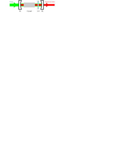
Figure 1: Linear cavity OPO with a quarter-wave plate. When rotated relatively to the principal axes of the type-II phase-matched crystal, this plate adds a linear coupling between orthogonally polarized signal and idler fields. Vacuum fluctuations can enter the system through the output mirror or the various losses.

We assume that the signal and idler modes are close to resonance and note $\Delta_{1}$ and $\Delta_{2}$ their small round trip phase detunings. The equations of motion for the classical field amplitudes – which are noted $A_{1}$ and $A_{2}$ for the signal and idler modes and $A_{0}$ for the pump – can be written as

$$\tau\frac{dA_{1}}{dt} = A_{1}(-\kappa^{\prime}+i\Delta_{1})+gA_{0}A_{2}^{\ast}+2i\rho e^{i(\theta-\psi)}A_{2}$$

$$\tau\frac{dA_{2}}{dt} = A_{2}(-\kappa^{\prime}+i\Delta_{2})+gA_{0}A_{1}^{\ast}+2i\rho e^{i(\psi-\theta)}A_{1}$$ (1)

where $\tau$ stands for the cavity round-trip time, $A_{0}^{in}$ for the input pump amplitude and $g$ for the parametric gain. $\theta$ and $\psi$ are respectively the birefringent phase shift introduced by the crystal and by the waveplate. The last term of these equations corresponds to the linear coupling induced by the rotated plate.

We will only consider the case where $\Delta_{1}=\Delta_{2}=2\rho$ and $\theta=\psi$. At this operating point the threshold is minimum longcham1 . In this case, the equations of motion are simpler and are written

$$\tau\frac{dA_{1}}{dt} = A_{1}(-\kappa^{\prime}+2i\rho)+gA_{0}A_{2}^{\ast}+2i\rho A_{2}$$

$$\tau\frac{dA_{2}}{dt} = A_{2}(-\kappa^{\prime}+2i\rho)+gA_{0}A_{1}^{\ast}+2i\rho A_{1}$$ (2)

A non-zero stationary solution exists if and only if the pump power $A_{0}$, taken real, exceeds the threshold power equal to $\frac{\kappa^{\prime}}{g}$. We define a reduced pumping parameter $\sigma$ equal to the input pump amplitude normalized to the threshold. The below threshold regime corresponds to $\sigma<1$.

These equations are linearized around the stationary values by setting $A_{i}=\overline{A_{i}}+\delta A_{i}$. In the below threshold regime, the mean value of $A_{1}$ and $A_{2}$ are zero. The linearized equations can then be written

$$-\frac{\tau}{\kappa^{\prime}}\frac{d(\delta A_{1})}{dt} = \delta A_{1}(1-ic)-\sigma\delta A_{2}^{\ast}-ic\delta A_{2}$$

$$-\frac{\sqrt{2\kappa}}{\kappa^{\prime}}\delta A_{1}^{in}-\frac{\sqrt{2\mu}}{\kappa^{\prime}}\delta B_{1}^{in}$$

$$-\frac{\tau}{\kappa^{\prime}}\frac{d(\delta A_{2})}{dt} = \delta A_{2}(1-ic)-\sigma\delta A_{1}^{\ast}-ic\delta A_{1}$$ (3)

$$-\frac{\sqrt{2\kappa}}{\kappa^{\prime}}\delta A_{2}^{in}-\frac{\sqrt{2\mu}}{\kappa^{\prime}}\delta B_{2}^{in}$$

where $c=\frac{2\rho}{\kappa^{\prime}}$. $\delta A_{i}^{in}$ and $\delta B_{i}^{in}$ correspond to the vacuum fluctuations entering the cavity due respectively to the coupling mirror and to the losses.

One can note that the fluctuations of the pump are not coupled to the signal and idler modes in the below threshold regime. It is obviously not the case above threshold and this point can explain in particular why the experimental observation above threshold of phase anti-correlations below the standard quantum limit is a difficult task laurat04d .

II.2 Variances

The fluctuations can be evaluated by taking the Fourier transform of the previous equations which leads to algebraic equations. We introduce the parameter $\Omega=\frac{\omega\tau}{2\kappa^{\prime}}=\frac{\omega}{\Omega_{c}}$, which is the noise frequency normalized to the cavity bandwidth $\Omega_{c}$. In the Fourier domain, the equations become

$$(1-ic+2i\Omega)\delta\widetilde{A_{1}}(\Omega)-\sigma\delta\widetilde{A_{2}^{\ast}}(-\Omega)-ic\delta\widetilde{A_{2}}(\Omega)-$$

$$\frac{\sqrt{2\kappa}}{\kappa^{\prime}}\delta\widetilde{A_{1}^{in}}(\Omega)-\frac{\sqrt{2\mu}}{\kappa^{\prime}}\delta\widetilde{B_{1}^{in}}(\Omega)=0\qquad$$

$$(1-ic+2i\Omega)\delta\widetilde{A_{2}}(\Omega)-\sigma\delta\widetilde{A_{1}^{\ast}}(-\Omega)-ic\delta\widetilde{A_{1}}(\Omega)-$$

$$\frac{\sqrt{2\kappa}}{\kappa^{\prime}}\delta\widetilde{A_{2}^{in}}(\Omega)-\frac{\sqrt{2\mu}}{\kappa^{\prime}}\delta\widetilde{B_{2}^{in}}(\Omega)=0\qquad$$ (4)

From these equations and their conjugates, one can determine the variance spectra of the signal and idler modes and their correlations. We define the fluctuations of the modes $A_{i}$ for a given quadrature angle $\varphi$ and a given noise frequency $\Omega$ by

$$p_{i}(\varphi)=\delta\widetilde{A_{i}}(\Omega)e^{-i\varphi}+\delta\widetilde{A_{i}^{\ast}}(-\Omega)e^{i\varphi}$$ (5)

The equation of motion for the fluctuations can thus take the following form

$$(1+2i\Omega)p_{1}(\varphi)-\sigma p_{2}(-\varphi)+c(p_{1}(\varphi+\pi/2)$$

$$+p_{2}(\varphi+\pi/2))-\frac{\sqrt{2\kappa}}{\kappa^{\prime}}p_{1}^{in}-\frac{\sqrt{2\mu}}{\kappa^{\prime}}p_{1}^{in^{\prime}} = 0$$

$$p_{2}(-\varphi)(1+2i\Omega)-\sigma p_{1}(\varphi)+c(p_{2}(-\varphi+\pi/2)$$

$$-p_{1}(-\varphi+\pi/2))-\frac{\sqrt{2\kappa}}{\kappa^{\prime}}p_{2}^{in}-\frac{\sqrt{2\mu}}{\kappa^{\prime}}p_{2}^{in^{\prime}} = 0$$ (6)

where $p_{i}^{in}$ and $p_{i}^{in^{\prime}}$ correspond to the phase-insensitive vacuum fluctuations entering the system.

When $c=0$, these equations are identical to the ones of a traditional type II OPO below threshold where only the quadratures with phases $\pm\varphi$ can interact. When the plate is rotated, the phase dependence becomes more complicated since orthogonal quadratures are coupled.

Figure 2: Angle of the minimal noise quadrature and corresponding normalized variance as a function of the coupling parameter. Close to $c=0$, the noise diverges and is phase-insensitive. $\Omega=0,\sigma=0.9,\kappa=\kappa^{\prime}$.

By introducing the simplified notations

$$p_{1}=p_{1}\Big{(}\varphi_{1}\Big{)} \qquad q_{1}=p_{1}\Big{(}\varphi_{1}+\frac{\pi}{2}\Big{)}$$ (7)

$$p_{2}=p_{2}\Big{(}\varphi_{2}\Big{)} \qquad q_{2}=p_{2}\Big{(}\varphi_{2}+\frac{\pi}{2}\Big{)}$$

with $\varphi_{1}=\pi/2$ and $\varphi_{2}=-\pi/2$, the equations of motion can be rewritten in the form

$$(1+2i\Omega)p_{1}-\sigma p_{2}+c(q_{1}-q_{2})$$

$$-\frac{\sqrt{2\kappa}}{\kappa^{\prime}}p_{1}^{in}-\frac{\sqrt{2\mu}}{\kappa^{\prime}}p_{1}^{in^{\prime}} = 0$$

$$p_{2}(1+2i\Omega)-\sigma p_{1}+c(q_{2}-q_{1})$$

$$-\frac{\sqrt{2\kappa}}{\kappa^{\prime}}p_{2}^{in}-\frac{\sqrt{2\mu}}{\kappa^{\prime}}p_{2}^{in^{\prime}} = 0$$

$$q_{1}(1+2i\Omega)+\sigma q_{2}+c(p_{2}-p_{1})$$

$$-\frac{\sqrt{2\kappa}}{\kappa^{\prime}}q_{1}^{in}-\frac{\sqrt{2\mu}}{\kappa^{\prime}}q_{1}^{in^{\prime}} = 0$$

$$q_{2}(1+2i\Omega)+\sigma q_{1}+c(p_{1}-p_{2})$$

$$-\frac{\sqrt{2\kappa}}{\kappa^{\prime}}q_{2}^{in}-\frac{\sqrt{2\mu}}{\kappa^{\prime}}q_{2}^{in^{\prime}} = 0$$ (8)

The system made up of these 4 equations and the 4 equations obtained by changing $\Omega$ in $-\Omega$ gives the intra-cavity fluctuations. The fluctuations of the output modes are obtained by the boundary condition on the output mirror

$$p_{i}^{out}(\Omega)=\sqrt{2\kappa}p_{i}(\Omega)-p_{i}^{in}$$ (9)

The variances of a component $p_{i}^{out}$ is then derived from

$$S_{p_{i}^{out}}(\Omega)=<p_{i}^{out}(\Omega)\,p_{i}^{out}(-\Omega)>$$ (10)

The variances of the uncorrelated vacuum contributions entering the system are normalized to 1.

II.3 Signal and idler fluctuations

When the plate is not rotated ($c=0$), the signal and idler modes exhibit phase-insensitive excess noise. The single-beam noise spectrum for the signal (or the idler) can be written

$$S_{p_{1}}=S_{q_{1}}=1+\frac{8\sigma^{2}}{(4\Omega^{2}+(\sigma-1)^{2})(4\Omega^{2}+(\sigma+1)^{2})}\frac{\kappa}{\kappa^{\prime}}$$ (11)

It is not the case when the plate is rotated. The noise becomes phase-sensitive and the noise spectrum is given by

$$S(\varphi)=S_{p_{1}}\cos(\varphi)^{2}+S_{q_{1}}\sin(\varphi)^{2}+\alpha\cos(2\varphi)$$ (12)

with

$$S_{p_{1}} = 1+\frac{8\sigma(\sigma((\sigma-1)^{2}+4\Omega^{2})-c^{2}(4\Omega^{2}-4(1+c^{2})+(\sigma+1)^{2})}{(4\Omega^{2}+(\sigma-1)^{2})(16\Omega^{2}+(4\Omega^{2}-4c^{2}+\sigma^{2}-1)^{2})}\frac{\kappa}{\kappa^{\prime}}$$

$$S_{q_{1}} = 1+\frac{8\sigma(\sigma((\sigma+1)^{2}+4\Omega^{2})+c^{2}(4\Omega^{2}-4(1+c^{2})+(\sigma-1)^{2})}{(4\Omega^{2}+(\sigma+1)^{2})(16\Omega^{2}+(4\Omega^{2}-4c^{2}+\sigma^{2}-1)^{2})}\frac{\kappa}{\kappa^{\prime}}$$

$$\alpha = \frac{-8\sigma c}{16\Omega^{2}+(4\Omega^{2}-4c^{2}+\sigma^{2}-1)^{2}}\frac{\kappa}{\kappa^{\prime}}$$ (13)

Figure 2 shows the evolution of the minimal noise quadrature angle and of the corresponding noise power as a function of the coupling parameter. When the coupling parameter $c$ increases, this quadrature rotates. For strong coupling, the minimal noise quadrature is closer and closer to the quadrature $q_{1}$ and $q_{2}$ and the noise can be squeezed well below the standard quantum limit.

II.4 Correlations and anti-correlations

After considering the individual fluctuations of signal and idler modes, we study here the intermodal correlations.

Let us introduce the superposition modes oriented $\pm 45^{\circ}$ from the axes of the crystal

$$A_{+}=\frac{A_{1}+A_{2}}{\sqrt{2}}\qquad\textrm{and}\qquad A_{-}=\frac{A_{1}-A_{2}}{\sqrt{2}}$$

It should be stressed that considering the noise spectrum of the sum or difference of signal and idler fluctuations is equivalent to considering the noise spectrum of the rotated modes. If signal and idler exhibit correlations or anti-correlations, these two modes can have squeezed fluctuations as their noise spectra are given by

$$S_{A_{+}}(\varphi)=\frac{1}{2}S_{p_{1}(\varphi)+p_{2}(\varphi)}\quad\textrm{and}\quad S_{A_{-}}(\varphi)=\frac{1}{2}S_{p_{1}(\varphi)-p_{2}(\varphi)}$$

The amount of entanglement between signal and idler can be directly inferred from the amount of squeezing available on these superposition modes.

The expressions for the anti-correlations between signal and idler modes coincide with the ones obtained in the case of a standard OPO below threshold

$$S_{q_{1}+q_{2}} = 1-\frac{4\sigma}{4\Omega^{2}+(\sigma+1)^{2}}\frac{\kappa}{\kappa^{\prime}}$$

$$S_{p_{1}+p_{2}} = 1+\frac{4\sigma}{4\Omega^{2}+(\sigma-1)^{2}}\frac{\kappa}{\kappa^{\prime}}$$ (14)

The combination $(q_{1}+q_{2})$ is always squeezed below the standard quantum limit while $(p_{1}+p_{2})$ is very noisy. Perfect anti-correlations are found at exact threshold in the absence of additional losses ($\kappa=\kappa^{\prime}$) and at zero frequency.

In contrast with the anti-correlations, the correlations largely depend on the presence of the plate. The variance spectrum is found to be

$$S_{A_{-}}(\varphi)=S_{p_{1}-p_{2}}\cos(\varphi)^{2}+S_{q_{1}-q_{2}}\sin(\varphi)^{2}+2\alpha\cos(2\varphi)$$ (15)

where $\alpha$ has been defined in Eq. (13) and

$$S_{p_{1}-p_{2}} = 1-\frac{4\sigma(4\Omega^{2}-4c^{2}+(\sigma-1)^{2})}{16\Omega^{2}+(4\Omega^{2}-4c^{2}+\sigma^{2}-1)}\frac{\kappa}{\kappa^{\prime}}$$

$$S_{q_{1}-q_{2}} = 1+\frac{4\sigma(4\Omega^{2}-4c^{2}+(\sigma+1)^{2})}{16\Omega^{2}+(4\Omega^{2}-4c^{2}+\sigma^{2}-1)}\frac{\kappa}{\kappa^{\prime}}$$ (16)

In a standard OPO below threshold – without a linear coupling – the correlated quadratures are orthogonal to the anti-correlated ones. It is not anymore the case when a coupling is introduced. The evolution is depicted in Fig. 3. When the plate angle increases, the correlated quadratures rotates and the correlations are degraded.

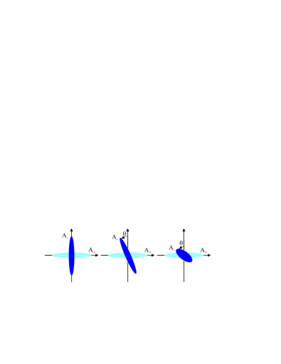
Figure 3: Fresnel representation of the noise ellipse of the $\pm 45^{\circ}$ rotated modes when the plate angle is increased. Without coupling, squeezing is predicted on orthogonal quadratures. The noise ellipse of the $-45^{\circ}$ mode rotates and the noise reduction is degraded when the coupling increases while the $+45^{\circ}$ rotated mode is not affected.

We can derive from Eqs (15) and (II.4) a simple expression for the tilt angle $\theta$ of the noise ellipse

$$\tan(2\theta)=\frac{4c}{4\Omega^{2}-4c^{2}+\sigma^{2}+1}$$ (17)

Figure 4 gives the tilt angle of the noise ellipse and the noise variance of the squeezed quadrature as a function of the coupling parameter.

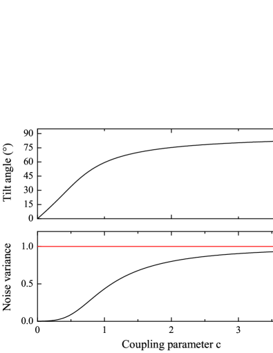
Figure 4: Angle $\theta$ of the minimal noise quadrature and corresponding normalized variance as a function of the coupling parameter $c$. $\Omega=0,\sigma=0.9,\kappa=\kappa^{\prime}$.

As a first conclusion, optimal correlations and anti-correlations are observed on non-orthogonal quadratures depending on the plate angle. In order to maximize the entanglement between the signal and idler modes, the optimal quadratures have to be made orthogonal Wolf . Such an operation consists in a phase-shift of $A_{-}$ relative to $A_{+}$. This transformation is thus ”non-local” in the sense of the EPR argument: it involves the two considered modes, signal and idler, and therefore has to be performed before spatially separating them.

$$\Gamma_{A_{1}\,\!A_{2}}=\left(\begin{array}[]{cc|cc}181.192&0&179.808&-0.255\\ 0&0.386&-0.255&-0.383\\ \hline\cr 179.808&-0.255&181.192&0\\ -0.255&-0.383&0&0.386\end{array}\right) \Longrightarrow \Gamma^{\prime}_{A_{1}\,\!A_{2}}=\left(\begin{array}[]{cc|cc}180.839&0&180.161&0\\ 0&0.739&0&-0.736\\ \hline\cr 180.161&0&180.839&0\\ 0&-0.736&0&0.739\end{array}\right)$$ (26)

$$\Gamma_{A_{+}\,\!A_{-}}=\left(\begin{array}[]{cc|cc}361&0&0&0\\ 0&0.00277&0&0\\ \hline\cr 0&0&1.383&-0.256\\ 0&0&-0.256&0.770\end{array}\right) \Longrightarrow \Gamma^{\prime}_{A_{+}\,\!A_{-}}=\left(\begin{array}[]{cc|cc}361&0&0&0\\ 0&0.00277&0&0\\ \hline\cr 0&0&0.677&0\\ 0&0&0&1.476\end{array}\right)$$ (35)

Figure 5: Numerical example of covariance matrix of the $A_{1}$/$A_{2}$ modes and the $A_{+}$/$A_{-}$ modes before and after the non-local operation for a coupling parameter $c=1.5$. ($\sigma=0.9,\Omega=0,\kappa=\kappa^{\prime}$)

II.5 In terms of covariance matrix

The behavior of the system and the optimization of the degree of entanglement can be formulated in terms of covariance matrix. We recall that a two-mode gaussian state with zero mean value is fully described by the covariance matrix $\Gamma_{A\,\!B}$ defined as

$$\Gamma_{A\,\!B}=\left(\begin{array}[]{cc}\gamma_{A}&\sigma_{A\,\!B}\\ \sigma_{A\,\!B}^{T}&\gamma_{B}\end{array}\right)$$

$\gamma_{A}$ and $\gamma_{B}$ are the covariance matrix of the individual modes while $\sigma_{A\,\!B}$ describes the intermodal correlations. The elements of the covariance matrix are written $\Gamma_{ij}=\langle\delta R_{i}\delta R_{j}+\delta R_{j}\delta R_{i}\rangle/2$ where $R_{\{i,i=1,..,4\}}=\{X_{A},Y_{A},X_{B},Y_{B}\}$. $X$ and $Y$ corresponds to an arbitrary orthogonal basis of quadratures.

In order to measure the degree of entanglement of Gaussian states, a simple computable formula of the logarithmic negativity $E_{\mathcal{N}}$ has been obtained in Ref. vidal (see also Adesso for a general overview). $E_{\mathcal{N}}$ can be easily evaluated from the largest positive symplectic eigenvalue $\xi$ of the covariance matrix which can be obtained from

$$\xi^{2}=\frac{1}{2}(D-\sqrt{D^{2}-4\det\Gamma_{A\,\!B}}\,)$$ (36)

with

$$D=\det\gamma_{A}+\det\gamma_{B}-2\det\sigma_{A\,\!B}$$ (37)

The two-mode state is entangled if and only if $\xi<1$. The logarithmic negativity can thus be expressed by $E_{\mathcal{N}}=-\log_{2}(\xi)$. This measurement is monotone and can not increase under LOCC (local operations and classical communications). The maximal entanglement which can be extracted from a given two-mode state by passive operations is related to the two smallest eigenvalues of $\Gamma$, $\lambda_{1}$ and $\lambda_{2}$, by $E_{\mathcal{N}}^{max}=-\log_{2}(\lambda_{1}\lambda_{2})/2$ Wolf .

Phase-shifting of $A_{+}$ and $A_{-}$ into $A_{+}\,e^{i\theta/2}$ and $A_{-}\,e^{-i\theta/2}$ corresponds to a transformation of the signal and idler modes $A_{1}$ and $A_{2}$ described by the matrix

$$M=\left(\begin{array}[]{cc}\cos(\theta/2)&i\sin(\theta/2)\\ i\sin(\theta/2)&\cos(\theta/2)\\ \end{array}\right)$$

The angle $\theta$ is given by Eq.(17). Such a transformation couples the signal and idler modes.

We give here a numerical example for realistic experimental values $c=1.5,\sigma=0.9$ and $\Omega=0$. The covariance matrix for the $A_{1}$/$A_{2}$ modes and also for the $A_{+}$/$A_{-}$ modes are given in Fig. 5 with and without the phase-shift. The matrix of the $A_{+}$/$A_{-}$ modes are well-suited to understand the behavior of the device. At first, the intermodal blocks are zero, showing that these two modes are not at all correlated and consequently are the most squeezed modes of the system. There is no way to extract more squeezing. But one can also note that the diagonal blocks are not diagonalized simultaneously. This corresponds to the tilt angle $\theta$ of the squeezed quadrature of $A_{-}$ and given by Eq. (17). A phase-shift of the angle $\theta$ permits to diagonalize simultaneously the two blocks and to obtain squeezing on orthogonal quadratures. From the matrix on the $A_{1}$/$A_{2}$ modes, one can quantify the degree of entanglement by the logarithmic negativity $E_{\mathcal{N}}$. Thanks to the non-local operation, $E_{\mathcal{N}}$ goes from $4.06$ to $4.53$. The maximal entanglement available has been extracted as $E_{\mathcal{N}}^{max}=-\log_{2}(\lambda_{1}\lambda_{2})/2=4.53$. Let us finally note that due to the strong coupling the signal and idler modes are entangled but also slightly squeezed.

A self-phase locked OPO below threshold can generate very strong entangled modes when the plate angle is small enough. The quantum behavior of the device is very rich and gives a good insight into two-mode gaussian state properties and entanglement characterization. The previous interpretation in terms of covariance matrix establishes a link between the optimal entanglement that can be extracted and the eigenvalues of the matrix. The way to find it by a non-local operation is developed. The next section is devoted to the experimental study of this original device.

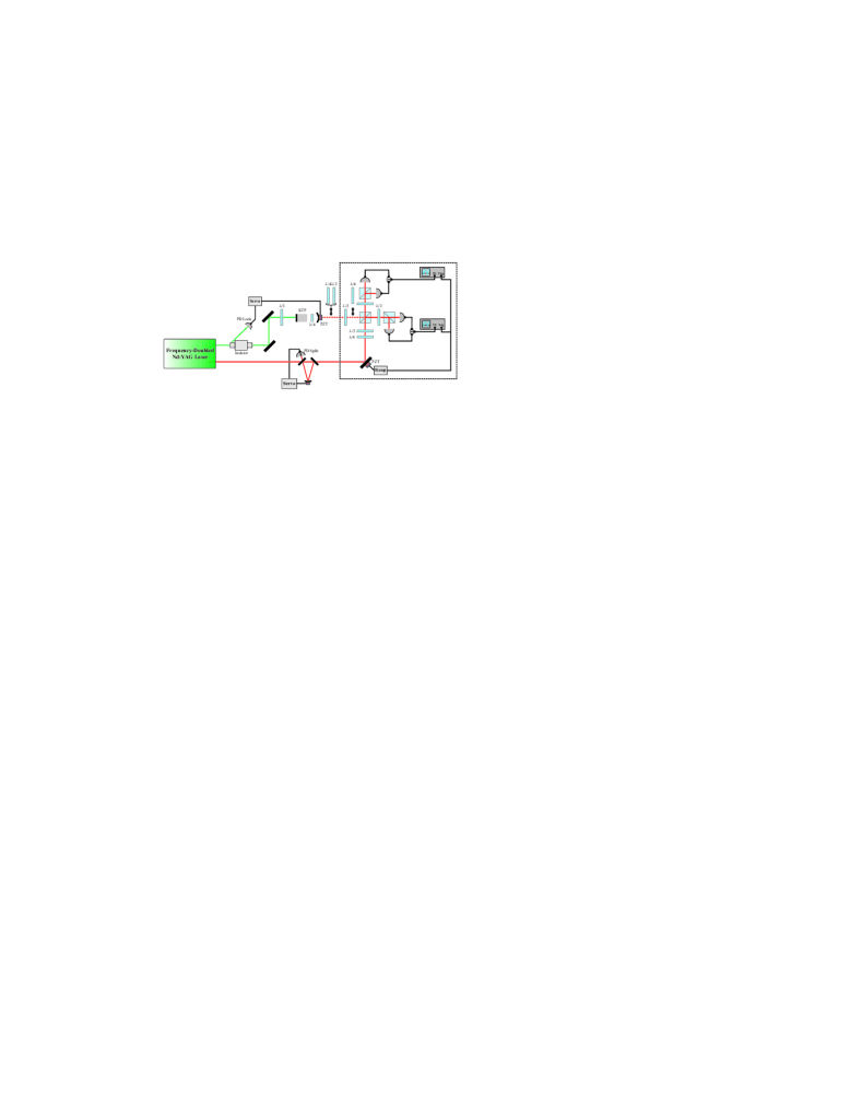
Figure 6: Experimental setup. A continuous-wave frequency-doubled Nd:YAG laser pumps below threshold a type II OPO with a $\lambda/4$ plate inserted inside the cavity. The generated two-mode vacuum state is characterized by two simultaneous homodyne detections. The infrared output of the laser is used as local oscillator after filtering by a high-finesse cavity. The two couples $\{\lambda/4,\lambda/2\}$ on each path are used to make arbitrary phase shift between orthogonal components of polarization. PD Lock: FND-100 photodiode for locking of the OPO. PD Split: split two-element InGaAs photodiode for tilt-locking of the filtering cavity.

III Experimental setup

Our experimental setup is based on a frequency degenerate type II OPO below threshold. A $\lambda/4$ plate inserted within the OPO adds a linear coupling between the signal and idler modes which depends on the angle of the plate relative to the principal axes of the crystal . Two simultaneous homodyne detections are implemented.

III.1 OPO and linear coupling

The experimental setup is shown in Fig. 6. A continuous frequency-doubled Nd:YAG laser (”Diabolo” without ”noise eater option”, Innolight GmbH) pumps a triply resonant type II OPO, made of a semi-monolithic linear cavity : in order to increase the mechanical stability and reduce the reflection losses, the input flat mirror is directly coated on one face of the 10mm-long KTP crystal ($\theta=90^{\circ}$, $\varphi=23.5^{\circ}$, Raicol Crystals Ltd.). The reflectivities for the input coupler are 95% for the pump (532nm) and almost 100% for the signal and idler beams (1064nm). The output coupler (R=38mm) is highly reflecting for the pump and its transmission is 5% for the infrared. At exact triple resonance, the oscillation threshold is less than 20 mW, very close to the threshold without the plate laurat03 . The OPO is actively locked on the pump resonance by the Pound-Drever-Hall technique: a remaining 12MHz modulation present in the laser is detected by reflection and the error signal is sent to a home-made PI controller. The crystal temperature is thoroughly controlled within the mK range. The OPO can operate stably during more than one hour without mode-hopping.

The birefringent plate inserted inside the cavity is chosen to be exactly $\lambda/4$ at 1064 nm and almost $\lambda$ at the 532 nm pump wavelength. As birefringence and dispersion are of the same order, this configuration is only possible by choosing multiple-order plate: we have chosen the first order for which exact $\lambda/4$ at 1064 nm is obtained, i.e. $4.75\lambda$ at 1064 nm and $9.996\lambda$ at 532 nm. Very small rotations of this plate around the cavity axis can be operated thanks to a rotation mount controlled by piezo-electric actuator (New Focus Model 8401 and tiny pico-motor).

III.2 Two simultaneous homodyne detections

The coherent 1064 nm laser output is used as local oscillator for homodyne detection. This beam is spatially filtered and intensity-noise cleaned by a triangular-ring 45 cm-long cavity with a high finesse of 3000. This cavity is locked on the maximum of transmission by the single-pass tilt-locking technique Shaddock and 80% of transmission is obtained. The homodyne detections are based on pairs of balanced high quantum efficiency InGaAs photodiodes (Epitaxx ETX300 with a 95% quantum efficiency) and the fringe visibility reaches 0.97. The shot noise level of all measurements is easily obtained by blocking the output of the OPO.

Orthogonally polarized modes are separated on the first polarizing beam splitter at the output of the OPO. A half-wave plate inserted before this polarizing beam splitter enables us to choose the fields to characterize: the signal and idler modes which are entangled, or the $\pm 45^{\circ}$ rotated modes which are squeezed.

One main requirement of our experiment is to be able to characterize simultaneously two modes with the same phase reference. The difference photocurrents of the homodyne detections are sent into two spectrum analyzers (Agilent E4411B) which are triggered by the same signal. The two homodyne detections are calibrated in order to be in phase: if one send into each detection a state of light with squeezing on the same quadrature, the noise powers registered on the spectrum analyzers must have in-phase variations while scanning the local oscillator phase. Two birefringent plates, $\lambda/2$ and $\lambda/4$, inserted in the local oscillator path are rotated in order to compensate residual birefringence due in particular to defects associated to polarizing beam splitter. In others words, after this correction, the polarization of the local oscillator is slightly elliptical. To facilitate this tuning, the OPO is operated above threshold in the locking zone where frequency degeneracy occurs. A polarizing beam splitter inserted at the OPO output and a $\lambda/2$ plate rotated by $22.5^{\circ}$ permit to send into the two homodyne detections states of light with opposite phase. Then, we look at the DC interference fringes which have to be in opposition. We check this calibration by sending into the homodyne detections a squeezed vacuum. When scanning the local oscillator phase, the noise variance measured in each homodyne detection follow simultaneous variations. A $\lambda/4$ plate can be added on the beam exiting the OPO, just before the homodyne detections: when this plate is inserted, the homodyne detections are in quadrature. In such a configuration, two states of light with squeezing on orthogonal quadratures give in-phase squeezing curves on the spectrum analyzers.

IV Experimental entanglement

In this section, we report on the experimental results obtained for different values of the coupling parameter. As underlined before, we characterize the noise of the $\pm 45^{\circ}$ rotated modes which have squeezed fluctuations.

IV.1 Without linear coupling

In a first series of experiments, the plate angle is adjusted to be almost zero. This tuning can be done by looking at the individual noises which should be in that case phase-insensitive. Squeezing of the rotated modes is thus expected on orthogonal quadratures, as it is well-known for a standard OPO. Typical spectrum analyser traces while scanning the local oscillator phase are shown on Fig. 7. Normalized noise variances of the $\pm 45^{\circ}$ vacuum modes at a given noise frequency of 3.5 MHz are superimposed for in-phase and in-quadrature homodyne detections. One indeed observes, as expected, correlations and anti-correlations of the emitted modes on orthogonal quadratures.

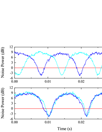
Figure 7: Normalized noise variances at 3.5 MHz of the $\pm 45^{\circ}$ modes while scanning the local oscillator phase. The first plot corresponds to in-phase homodyne detections and the second one in-quadrature. Squeezing is well observed on orthogonal quadratures. The resolution bandwidth is set to 100 kHz and the video bandwidth to 1 kHz.

Figure 8 gives the simultaneous measurement of the noise reductions for a locked local oscillator phase. $-4.3\pm 0.3$ dB and $-4.5\pm 0.3$ dB below the standard quantum limit are obtained for the two rotated modes. After correction of the electronic noise, the amounts of squeezing reach $-4.7\pm 0.3$ dB and $-4.9\pm 0.3$ dB. These values have to be compared to the theoretical value expressed in Eq. (II.4). By taking $\sigma=0.9$, $\Omega=0.1$, $\kappa=0.025$ and $\kappa^{\prime}=0.03$, the expected value before detection is $-7.5$ dB. The detector quantum efficiency is estimated to $0.95$, the fringe visibility is $0.97$ and the propagation efficiency is evaluated around $0.99$. These values give an overall detection efficiency of $0.95\cdot 0.97^{2}\cdot 0.99=0.88$. After detection, the expected squeezing is thus reduced to $-5.5$ dB. The small discrepancy with the experimental values can be due to the presence of walk-off which limits the modes overlap, a critical point for two-mode squeezing.

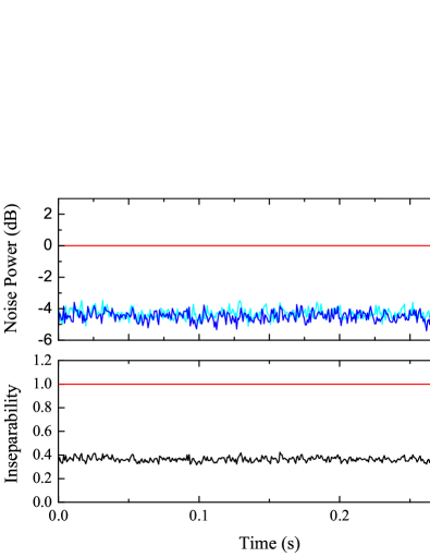
Figure 8: Normalized noise variances at 3.5 MHz of the $\pm 45^{\circ}$ modes and inseparability criterion for signal and idler modes. The homodyne detections are in-quadrature. After correction of the electronic noise, the inseparability criterion reaches $0.33\pm 0.02$. The resolution bandwidth is set to 100 kHz and the video bandwidth to 300 Hz.

From the electronic noise corrected squeezing values, one can infer the Duan and Simon inseparability criterion defined as the half sum $\Delta$ of the squeezed variances duan ; simon . For a symmetric gaussian two-mode state, this criterion is a necessary and sufficient condition of non-separability. We obtained a value of $\Delta=0.33\pm 0.02$ well below the unit limit for inseparability. It is worth noting that the simultaneous double homodyne detection permits a direct and instantaneous verification of this criterion by adding the two squeezed variances.

The EPR criterion is related to an apparent violation of a Heisenberg inequality reid : the information extracted from the measurement of the two quadratures of one mode provides values for the quadratures of the other mode that violate the Heisenberg inequality. This criterion is related to the product of conditional variances: $V_{P_{1}|P_{2}}\,V_{Q_{1}|Q_{2}}<1$ where $P_{i}$ et $Q_{i}$ are two conjugate quadratures and $V_{X_{1}|X_{2}}$ the conditional variance of $X_{1}$ knowing $X_{2}$. The knowledge of the previous squeezed quadratures and of the individual noise of the entangled modes give the conditional variances. The noise of signal and idler modes are phase-insensitive and reach $8.2\pm 0.5$ dB above shot noise (fig. 11). We obtained thus a product of conditional variances equal to $0.42\pm 0.05$, which confirms the EPR character of the measured correlations.

The entanglement can be quantified by the entropy of formation – or entanglement of formation $EOF$ – for symmetric gaussian states introduced in Ref.giedke , which represents the amount of pure state entanglement needed to prepare the entangled state. This entropy can be directly derived from the inseparability criterion value $\Delta$ by

$$EOF=c_{+}\log_{2}(c_{+})-c_{-}\log_{2}(c_{-})$$ (38)

with

$$c_{\pm}=(\Delta^{-1/2}\pm\Delta^{1/2})^{2}/4$$ (39)

From this expression, we calculate an entanglement of formation value of $EOF=1.1\pm 0.1\,ebits$. To the best of our knowledge, our setup generates the best EPR entangled beams to date produced in the continuous variable regime. Let us note that such a degree of entanglement should correspond to a fidelity equal to $0.75$ in a unity gain teleportation experiment.

This non-classical behavior exists also without the plate and we have obtained in that case almost the same degree of entanglement. The first experimental demonstration of continuous variable EPR entanglement was obtained with such a type II OPO below threshold Ou . However, the linear coupling – even for a plate rotated by a very small angle – can make easier the finding of experimental parameters for which entanglement is observed. Furthermore, the degenerate operation with bright beams above threshold makes possible to match the homodyne detection without infrared injection of the OPO.

The entanglement of the generated two-mode state is preserved for very low noise frequencies, down to 50 kHz. In the experimental quantum optics field, non-classical properties are generally reported in the MHz range – as it is the case in this paper up to now – due to large classical excess noise at lower frequencies. Experimental details and possible applications of this low frequency results are reported in laurat04b .

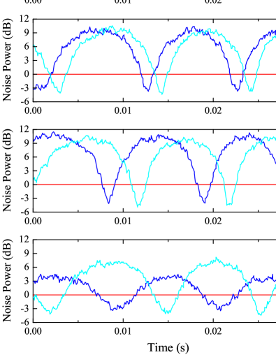
Figure 9: Normalized noise variances at 3.5 MHz of the $\pm 45^{\circ}$ modes while scanning the local oscillator phase for different coupling parameters: (a) $c=0$, (b) $c=0.35$, (c) $c=0.85$ and (d) $c=1.8$. Dark lines correspond to the $A_{-}$ mode and light ones to the $A_{+}$ mode. The homodyne detections are in-quadrature. The resolution bandwidth is set to 100 kHz and the video bandwidth to 1 kHz.

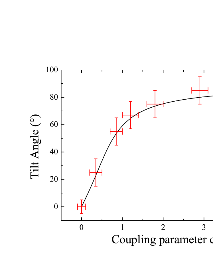
Figure 10: Measured tilt angle $\theta$ and noise variance as a function of the coupling parameter c, for the $A_{-}$ mode. The black lines give theoretical predictions calculated from Eq. (17) and (15) for $\sigma=0.9$ and $\Omega=0.1$.

IV.2 Results as a function of the linear coupling

The two-mode state generated by the self-phase-locked OPO is then characterized for different angles of the plate. We use the in-quadrature setup of the homodyne detections for which squeezing on orthogonal quadratures is observed simultaneously on the triggered spectrum analyzers. When the coupling increases, the squeezing is not obtained on orthogonal quadratures anymore. Figure 9 gives for four increasing coupling parameters the normalized noise variances of the rotated modes while scanning the local oscillator phase. In Fig. 10, we give the experimentally measured tilt angle $\theta$ and associated noise variance as a function of the coupling parameter $c$. One can check on the figure the validity of the theoretical expression of $\theta$ given in Eq. (17). We observe that the squeezing of the $A_{-}$ mode decreases but more slowly than expected. We also note that the squeezing of the $A_{+}$ mode slightly decreases while this noise reduction is theoretically independent of the coupling.

The noise of the signal and idler modes also depends on the presence of the plate as demonstrated in Sec. II. The individual noises become phase-sensitive, and even squeezed below the standard quantum limit, when the coupling increases. Figure 11 gives the phase dependance of the signal and idler modes for the same four coupling parameters than in Fig. 9.

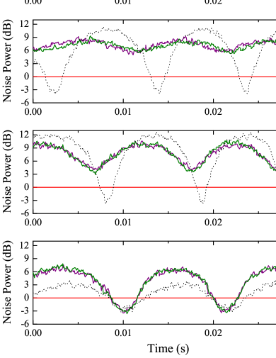
Figure 11: Normalized noise variances at 3.5 MHz of the signal and idler modes while scanning the local oscillator phase for different coupling parameters: (a) $c=0$, (b) $c=0.35$, (c) $c=0.85$ and (d) $c=1.8$. The black dotted lines correspond to the noise power on the difference of the two modes. The homodyne detections are in-phase. The resolution bandwidth is set to 100 kHz and the video bandwidth to 1 kHz.

IV.3 Optimization of EPR entanglement by polarization adjustement

When the plate is rotated, squeezing is not observed on orthogonal quadratures anymore. Thus, as shown in Sec.II, the EPR entanglement is not the maximal available one. In order to extract the maximal entanglement, one has to perform a phase-shift of the $A_{+}$ and $A_{-}$ modes. Such an arbitrary phase-shift can be done thanks to a couple of a $\lambda/2$ and a $\lambda/4$ plates added at the output of the OPO (Fig.6).

Figure 12 gives the normalized noise variances of the rotated modes for a coupling parameter $c=0.35$, before and after the phase-shift. The homodyne detections are operated in quadrature so that squeezing on orthogonal quadratures is observed simultaneously on the spectrum analyzers. After the operation performed, squeezing is obtained on orthogonal quadratures as in a standard type II OPO without coupling.

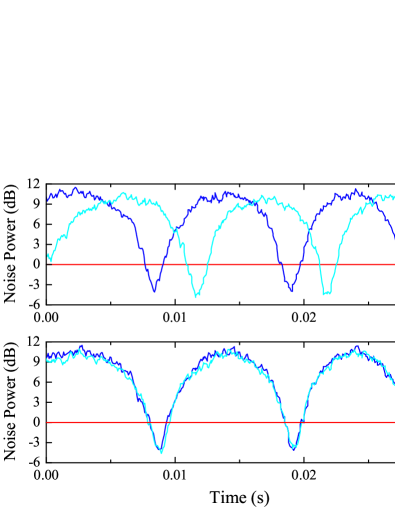
Figure 12: Normalized noise variances at 3.5 MHz of the rotated modes while scanning the local oscillator phase for a coupling parameter $c=0.35$, before and after the non-local operation. The homodyne detections are in-quadrature. After this operation, squeezing is observed on orthogonal quadratures. The resolution bandwidth is set to 100 kHz and the video bandwidth to 1 kHz.

V Conclusion

A self-phase-locked type II OPO associates to the usual non-linear coupling between the signal and idler modes a linear mixing by the way of a rotated quarter-wave plate inserted inside the optical cavity. We have demonstrated theoretically and confirmed experimentally that this original device generates a two-mode non-classical state that exhibits a very rich and interesting behavior in terms of squeezing and correlation properties. Quantum correlations and anti-correlations of the signal and idler modes are obtained on non-orthogonal quadratures depending on the angle of the plate. Furthermore, by a suitable change of polarization, the entanglement can be maximized and put into standard form, i.e. correlations and anti-correlations on orthogonal quadratures. The observed entanglement has been characterized in terms of covariance matrix and logarithmic negativity.

The experimental investigation of this original device required the setup of two simultaneous homodyne detections. We have detailed the operation of the system as a function of the coupling parameter – for the signal and idler modes which are entangled as well for the $\pm 45^{\circ}$ rotated modes which have squeezed fluctuations – and found the experimental behavior consistent with the theory. In the case of a very small coupling, we have reported what is to our knowledge the best entangled beams ever produced in the continuous variable regime. A value of the inseparability criterion as low as $0.33\pm 0.02$, well below the limit of unity, is obtained. This entanglement corresponds to a value of the entanglement of formation of $1.1\pm 0.1$ ebits. We also achieved EPR entanglement and squeezing at very low noise sideband frequencies down to 50 kHz laurat04b .

The next step is the characterization of the quantum properties of this system operated above threshold. The linear coupling induced by the plate results in a phase-locking of the signal and idler fields at frequency degeneracy, which permits to access the phase fluctuations of the bright twin beams. The predicted quantum properties of the system are similar and should open the possibility to generate bright entangled beams longcham2 . Up to now, phase-locking and intensity correlations below the standard quantum limit have been observed but the phase anticorrelations are still slightly above shot noise laurat04d . Improvements of the setup are currently in progress.

- (1) Quantum information with Continuous Variables, edited by S. L. Braunstein and A. K. Pati (Kluwer Academic Publishers, Dordrecht, 2003)
- (2) A. Furusawa, J.L. Sorensen, S.L. Braunstein, C.A. Fuchs, H.J. Kimble, E.S. Polzik, Science 282, 706 (1998)
- (3) W.P. Bowen, N. Treps, B.C. Buchler, R. Schnabel, T.C. Ralph, H. Bachor, T. Symul, P.K. Lam, Phys. Rev. A 67, 032302 (2003)
- (4) C. Silberhorn, N. Lütkenhaus, T.C. Ralph, G. Leuchs, Phys. Rev. Lett. 89, 4267 (2001)
- (5) V. Josse, A. Dantan, A. Bramati, M. Pinard, E. Giacobino, Phys. Rev. Lett. 92, 123601 (2004)
- (6) Z.Y. Ou, S.F. Pereira, H.J. Kimble, K.C. Peng, Phys. Rev. Lett. 68, 3663 (1992)
- (7) C. Schori, J.L. Sorensen, E.S. Polzik, Phys. Rev. A 66, 033802 (2002)
- (8) Y. Zhang, H. Wang, X. Li, J. Jing, C. Xie, K. Peng, Phys. Rev. A 62, 023813 (2000)
- (9) E. J. Mason, N. C. Wong, Opt. Lett. 23, 1733 (1998)
- (10) L. Longchambon, J. Laurat, T. Coudreau, C. Fabre, Eur. Phys. J. D 30, 279 (2004)
- (11) L. Longchambon, J. Laurat, T. Coudreau, C. Fabre, Eur. Phys. J. D 30, 287 (2004)
- (12) S. Reynaud, C. Fabre, E. Giacobino, J. Opt. Soc. Am. B 4, 1520 (1987)
- (13) J. Laurat, L. Longchambon, T. Coudreau, C. Fabre, in preparation
- (14) M.M. Wolf, J. Eisert, M.B. Plenio, Phys. Rev. Lett 90, 047904 (2003)
- (15) G. Vidal, R.F. Werner, Phys. Rev. A 65, 032314 (2002)
- (16) G. Adesso, A. Serafini, F. Illuminati, Phys. Rev. A 70, 022318 (2004)
- (17) J. Laurat, T. Coudreau, N. Treps, A. Maître, C. Fabre, Phys. Rev. Lett. 91, 213601 (2003)
- (18) D. A. Shaddock, M. B. Gray, D. E. McClelland, Opt. Lett. 24, 1499 (1999)
- (19) L.-M. Duan, G. Giedke, J. I. Cirac, P. Zoller, Phys. Rev. Lett 84, 2722 (2000)
- (20) R. Simon, Phys. Rev. Lett 84, 2726 (2000).
- (21) M.D. Reid, P. Drummond, Phys. Rev. Lett. 60, 2731 (1988)
- (22) G. Giedke, M.M. Wolf, O. Krüger, R.F. Werner, J.I. Cirac, Phys. Rev. Lett 91, 107901 (2003)
- (23) R. Schnabel, H. Vahlbruch, A. Franzen, S. Chelkowski, N. Grosse, H.-A Bachor, W.P. Bowen, P. K. Lam, K. Danzmann, Optics Communications 240, 185 (2004)
- (24) J. Laurat, T. Coudreau, G. Keller, N. Treps, C. Fabre, accepted for publication in Phys. Rev. A, e-print quant-ph/0403224