The Quantum Geometric Phase between Orthogonal States

Abstract

We show that the geometric phase between any two states, including orthogonal states, can be computed and measured using the notion of projective measurement, and we show that a topological number can be extracted in the geometric phase change in an infinitesimal loop near an orthogonal state. Also, the Pancharatnam phase change during the passage through an orthogonal state is shown to be either $\pi$ or zero (mod $2\pi$). All the off-diagonal geometric phases can be obtained from the projective geometric phase calculated with our generalized connection.

The existence of the geometric phase was first pointed out by Berry berry1984 in adiabatic systems and was later generalized to non-adiabatic cyclic aaphase and non-cyclic generalsetting cases, through the use of the Pancharatnam connection generalsetting ; pancharatnam in the latter case. However, the geometric phase between two orthogonal states is undefined in the Pancharatnam connection, even though orthogonal states do contain phase information, which could indeed be extracted for adiabatic evolution by calculating the off-diagonal geometric phases offdiag . The latter was generalized further to non-adiabatic situations by using the $N$-vertex Bargmann invariant mukunda2003 and to systems involving mixed-states Filipp and Sjoqvist (2003), and it was verified in various experiments such as microwave cavity offdiag and neutron interferometry Hasegawa et al. (2001, 2002).

We show in this article that the geometric phase between any two states, orthogonal or not, can be computed and measured in general using the concept of projective measurement. We find that the geometric phase change when a state evolves in an infinitesimal loop near an orthogonal state is associated with a topological number, and if the state actually evolves into an orthogonal state, the phase change is either $\pi$ or zero (mod $2\pi$). Our generalized connection can be used to calculate all phase information between two states; in particular, all the off-diagonal geometric phases can be obtained.

A physical interpretation of the Pancharatnam connection is that the initial state $\left|{\psi(0)}\right\rangle$ and final state $\left|\psi(t)\right\rangle$ (with the dynamical phases removed) are taken to interfere, and the amplitude $\langle\psi(t)|\psi(0)\rangle$ reflects the phase difference between the states. Following this idea, we can define another kind of interference by first projecting the initial and final states to a certain state $\left|i\right\rangle$, which gives $\left|i\right\rangle\left\langle{i}\mathrel{\left|{\vphantom{i{\psi(0)}}}\right.\kern-1.2pt}{{\psi(0)}}\right\rangle$ and $\left|i\right\rangle\left\langle{i}\mathrel{\left|{\vphantom{i{\psi(t)}}}\right.\kern-1.2pt}{{\psi(t)}}\right\rangle$. Then they are taken to interfere, giving a projective phase defined up to an arbitrary phase of $2n\pi$,

$$\varphi_{i}(0,t)=\arg\left\langle{{\psi(0)}}\mathrel{\left|{\vphantom{{\psi(0)}i}}\right.\kern-1.2pt}{i}\right\rangle\left\langle{i}\mathrel{\left|{\vphantom{i{\psi(t)}}}\right.\kern-1.2pt}{{\psi(t)}}\right\rangle.$$ (1)

In particular, when the state $\left|i\right\rangle$ is taken to be the initial or final state, or some state along the geodesic, $\varphi_{i}(0,t)$ reduces to the Pancharatnam phase difference, $\arg\left\langle{{\psi(0)}}\mathrel{\left|{\vphantom{{\psi(0)}{\psi(t)}}}\right.\kern-1.2pt}{{\psi(t)}}\right\rangle.$

An example of this interference is that between the $x$-polarized light and the $y$-polarized light after directing them through a polarizer in the direction $\hat{x}+\hat{y}$. The result is physically measurable and is given by Eq. (1). The definition in Eq. (1) is independent of the choice of gauge of $\left|i\right\rangle$, since a projection operator, which is gauge invariant, is used in the definition.

Following the idea in generalsetting , the phase can be evaluated by defining two curves, the projections of which on the ray space are the shortest geodesics, $\phi_{1}(s_{1})$ and $\phi_{2}(s_{2})$, $0\leq s_{k}\leq 1$, $k=1,2$, which satisfy $\left|{\phi_{1}(0)}\right\rangle=\left|{\psi(t)}\right\rangle$, $\left|{\phi_{1}(1)}\right\rangle=\left|{\phi_{2}(0)}\right\rangle=\left|i\right\rangle$ and $\left|{\phi_{2}(1)}\right\rangle=\left|{\psi(0)}\right\rangle$. We have therefore

$$\varphi_{i}(0,t)=\int_{0}^{1}{A_{1}ds_{1}}+\int_{0}^{1}{A_{2}ds_{2}}$$

along the two geodesics, where

$$A_{k}={\mathop{\rm Im}\nolimits}\left\langle{\phi_{k}(s_{k})}\right|\frac{d}{{ds_{k}}}\left|{\phi_{k}(s_{k})}\right\rangle,$$

for $k=1,2$. Then a closed path $\gamma$ can be defined by the evolution path of the state and the two geodesics, and the phase in Eq. (1) can be evaluated by Stoke’s theorem, $\varphi_{i}(0,t)=\int_{S}F$, where $F$ is the two-form $dA$, and the integral is over the surface $S$ bounded by $\gamma$. Physically, we first parallel-transport the initial and final states to $\left|i\right\rangle$ and then compare them to obtain the phase difference.

Consider the projective measurements at two states, $|i\rangle$ and $|j\rangle$. The projective phases are given by

$$\begin{array}[]{l}\varphi_{i}(0,t)=\arg\left\langle{0}\mathrel{\left|{\vphantom{0i}}\right.\kern-1.2pt}{i}\right\rangle\left\langle{i}\mathrel{\left|{\vphantom{it}}\right.\kern-1.2pt}{t}\right\rangle,\\ \varphi_{j}(0,t)=\arg\left\langle{0}\mathrel{\left|{\vphantom{0j}}\right.\kern-1.2pt}{j}\right\rangle\left\langle{j}\mathrel{\left|{\vphantom{jt}}\right.\kern-1.2pt}{t}\right\rangle,\\ \end{array}$$ (2)

where $\left|t\right\rangle=\left|{\psi(t)}\right\rangle$, and their difference is,

$$\varphi_{i}(0,t)-\varphi_{j}(0,t)=\arg\left\langle{0}\mathrel{\left|{\vphantom{0i}}\right.\kern-1.2pt}{i}\right\rangle\left\langle{j}\mathrel{\left|{\vphantom{j0}}\right.\kern-1.2pt}{0}\right\rangle+\arg\left\langle{t}\mathrel{\left|{\vphantom{tj}}\right.\kern-1.2pt}{j}\right\rangle\left\langle{i}\mathrel{\left|{\vphantom{it}}\right.\kern-1.2pt}{t}\right\rangle.$$

We define the gauge transformation, or the transition function as,

$$S_{ij}(P)=S_{ji}^{-1}(P)=\frac{{\left\langle{j}\mathrel{\left|{\vphantom{jP}}\right.\kern-1.2pt}{P}\right\rangle\left\langle{P}\mathrel{\left|{\vphantom{Pi}}\right.\kern-1.2pt}{i}\right\rangle}}{{\left|{\left\langle{j}\mathrel{\left|{\vphantom{jP}}\right.\kern-1.2pt}{P}\right\rangle\left\langle{P}\mathrel{\left|{\vphantom{Pi}}\right.\kern-1.2pt}{i}\right\rangle}\right|}},$$ (3)

where $\left|P\right\rangle$ is a state not orthogonal to either $\left|i\right\rangle$ or $\left|j\right\rangle$. We therefore have the transformation,

$$\exp\left({i\varphi_{i}(0,t)}\right)=S_{ij}(0)\exp\left({i\varphi_{j}(0,t)}\right)S_{ji}(t).$$

$S_{ij}(P)$ depends locally on the state $\left|P\right\rangle$ in the ray space, as it appears as the projection operator $\left|P\right\rangle\left\langle P\right|$ in the definition. It satisfies the properties of the transition function of a fibre bundle, in regions where $S_{ij}$ is well-defined, i.e., $S_{ii}(P)=1$, $S_{ij}(P)S_{ji}(P)=1$ and $S_{ij}(P)S_{jk}(P)=S_{ik}(P)$.

We can also calculate the phase change in a segment of the evolution curve using the definition in Eq. (1),

$$\varphi_{i}(t_{1},t_{2})=\arg\left\langle{{t_{1}}}\mathrel{\left|{\vphantom{{t_{1}}i}}\right.\kern-1.2pt}{i}\right\rangle\left\langle{i}\mathrel{\left|{\vphantom{i{t_{2}}}}\right.\kern-1.2pt}{{t_{2}}}\right\rangle.$$ (4)

This allows us to have associativity not shared by the Pancharatnam connection,

$${\varphi_{i}(0,t)} = {\arg\left\langle{0}\mathrel{\left|{\vphantom{0i}}\right.\kern-1.2pt}{i}\right\rangle\left\langle{i}\mathrel{\left|{\vphantom{i{t_{1}}}}\right.\kern-1.2pt}{{t_{1}}}\right\rangle\left\langle{{t_{1}}}\mathrel{\left|{\vphantom{{t_{1}}i}}\right.\kern-1.2pt}{i}\right\rangle\left\langle{i}\mathrel{\left|{\vphantom{it}}\right.\kern-1.2pt}{t}\right\rangle}$$ (5)

$$= {\varphi_{i}(0,t_{1})+\varphi_{i}(t_{1},t)}.$$

When a path goes through a region between $t_{1}$ and $t_{2}$ where the projection on $\left|j\right\rangle$ is defined, but not that of $\left|i\right\rangle$, we can easily prove the associative property,

$$e^{i\varphi_{i}(0,t_{3})}=e^{i\varphi_{i}(0,t_{1})}S_{ij}(t_{1})e^{i\varphi_{j}(t_{1},t_{2})}S_{ji}(t_{2})e^{i\varphi_{i}(t_{2},t_{3})}.$$ (6)

The covering of $\left|i\right\rangle$ consists of all states not orthogonal to $\left|i\right\rangle$, and $\varphi_{i}(0,t)$ is well-defined when both $\left|\psi(0)\right\rangle$ and $\left|\psi(t)\right\rangle$ are inside the covering. When the covering is specified, the structure is a principal coordinate bundle Nakahara (1990), where the fibre is space of the projective phase, and the base is the ray space.

For a two-state system, the structure of the ray space is the same as that of a monopole Shapere and Wilczek (1989); Wu and Yang (1975). By the associative property of Eq. (5), we can write the projective phase as

$$\varphi_{i}(0,t)=\sum\limits_{m}{\arg\left\langle{{t_{m}}}\mathrel{\left|{\vphantom{{t_{m}}i}}\right.\kern-1.2pt}{i}\right\rangle\left\langle{i}\mathrel{\left|{\vphantom{i{t_{m+1}}}}\right.\kern-1.2pt}{{t_{m+1}}}\right\rangle}=\sum\limits_{m}{\int_{\Delta S}F},$$ (7)

where $t_{m+1}=t_{m}+\Delta t$ and $\Delta S$ is the surface bounded by two geodesics linking $i$ to $\psi(t)$ and $\psi(t+\Delta t)$ and the evolution path from $\psi(t)$ to $\psi(t+\Delta t)$. For a two-state system, let $\left|i\right\rangle=\left|\uparrow\right\rangle$, and we have,

$${\int_{\Delta S}F}=-\frac{1}{2}(1-\cos\theta)\Delta\phi,$$ (8)

where $\theta$, $\phi$ are the coordinates of the Bloch sphere and we have used the solid angle formula from berry1984 . We can define a vector potential, whose curl is $F$: $(A_{\phi})_{i}=-\frac{1}{2}(1-\cos\theta)$, and $(A_{\theta})_{i}=0.$ For $\left|j\right\rangle=\left|\downarrow\right\rangle$, $(A_{\phi})_{j}=\frac{1}{2}(1+\cos\theta)$, $(A_{\theta})_{j}=0$. The transition function is $S_{ij}(\theta,\phi)=\exp(i\phi)$, where $\left|{\theta,\phi}\right\rangle=\cos{\frac{\theta}{2}}e^{-i\phi/2}\left|\uparrow\right\rangle+\sin{\frac{\theta}{2}}e^{i\phi/2}\left|\downarrow\right\rangle$. The results are formally identical to Wu and Yang’s solution to the monopole problem Wu and Yang (1975).

From Eq. (7), we can write the geometric phase as a sum of Bargmann invariants,

$$\varphi_{i}(t,t+\Delta t) = \varphi_{B}(t,i,t+\Delta t)$$ (9)

$$= \arg\left\langle{t}\mathrel{\left|{\vphantom{ti}}\right.\kern-1.2pt}{i}\right\rangle\left\langle{i}\mathrel{\left|{\vphantom{i{t+\Delta t}}}\right.\kern-1.2pt}{{t+\Delta t}}\right\rangle\left\langle{{t+\Delta t}}\mathrel{\left|{\vphantom{{t+\Delta t}t}}\right.\kern-1.2pt}{t}\right\rangle.$$

The term $\arg\left\langle{{t+\Delta t}}\mathrel{\left|{\vphantom{{t+\Delta t}t}}\right.\kern-1.2pt}{t}\right\rangle$ is responsible for removing the dynamical phase, and it can be omitted if parallel transport is used. We can construct a path close to $\left|j\right\rangle$, represented by $\left|{\phi(\theta)}\right\rangle=U\left|j\right\rangle=e^{i\delta\hat{\lambda}(\theta)}\left|j\right\rangle$, where $\delta$ is a small number and $\hat{\lambda}$ is a hermitian operator. The geometric phase change along the path from $\theta_{1}$ to $\theta_{2}$ is,

$$\varphi_{i}(\theta_{1},\theta_{2}) = {\mathop{\rm Im}\nolimits}\int_{\theta_{1}}^{\theta_{2}}{\frac{{\left\langle{\phi}\mathrel{\left|{\vphantom{\phi i}}\right.\kern-1.2pt}{i}\right\rangle\left\langle i\right|\frac{d}{{d\theta}}\left|\phi\right\rangle}}{{\left|{\left\langle{\phi}\mathrel{\left|{\vphantom{\phi i}}\right.\kern-1.2pt}{i}\right\rangle}\right|^{2}}}}d\theta$$ (10)

$$= \arg\left.{\left\langle i\right|U\left|j\right\rangle}\right|_{\theta_{2}}-\arg\left.{\left\langle i\right|U\left|j\right\rangle}\right|_{\theta_{1}}.$$

On the other hand, the phase $\varphi_{j}(\theta_{1},\theta_{2})$ is zero since the path is infinitesimally close to $\left|j\right\rangle$, and so

$$\varphi_{i}(\theta_{1},\theta_{2})=\arg(S_{ij}(\theta_{2})S_{ji}(\theta_{1}))+2n\pi.$$ (11)

Therefore the phases of any two infinitesimal paths with equal end-points (in the ray space) can differ only by $2n\pi$. The phase $\varphi_{i}(\theta_{1},\theta_{2})$ is well-defined if and only if $z\equiv{\left\langle i\right|U\left|j\right\rangle}$ is not zero at every point on the path. From Eq. (10) we can treat the phase $\varphi_{i}$ as the winding number of $z$ in its complex plane, and if the path is smoothly deformed with end points fixed, the value of $\varphi_{i}$ is not changed, unless the deformed path of ${U\left|j\right\rangle}$ crosses a zero of $z$. These zeros naturally divide all paths near $\left|j\right\rangle$ connecting two fixed points into different classes corresponding to different phases. This shows that the phase difference ($2n\pi$) of different classes of paths is topological.

Although by measurement between two states only the modulo $2\pi$ phase can be measured, the topological part of the phase $2n\pi$ can be observed by accumulating the changes of the phase as a function of time, $\varphi_{i}(t_{1},t_{2})=\sum{d\varphi_{i}}/{dt}\Delta t$, borrowing the idea of continuous measurement of the Pancharatnam phase in Bhandari (2002). We can decompose a path into segments and measure the phase change as in Eq. (4). From this definition, the phase is well defined if the state does not evolve to a state orthogonal to $\left|i\right\rangle$ along the path.

If the end-points merge into one ($\theta_{2}\to\theta_{1}$), the infinitesimal path $U\left|j\right\rangle$ becomes a closed loop, and the set of geodesics from points on the loop to ${\left|j\right\rangle}$ defines a two-dimensional manifold $O_{j}$ that includes ${\left|j\right\rangle}$. As $z={\left\langle i\right|U\left|j\right\rangle}$ is non-zero, geodesics from ${U\left|j\right\rangle}$ to $\left|i\right\rangle$ are well-defined . The set of geodesics from ${U\left|j\right\rangle}$ to $\left|i\right\rangle$ forms a two-dimensional manifold $O_{i}$. $O_{i}$ and $O_{j}$ form an $S^{2}$ sphere, and the geometric phase is,

$$\varphi_{i}(\theta_{1},\theta_{2}) = 2n\pi=\oint{A_{i}}=\int_{O_{i}}{F_{i}}$$ (12)

$$\approx \int_{O_{i}}{F_{i}}+\int_{O_{j}}{F_{j}}=\int_{S^{2}}F,$$

where we have used the the approximation that $O_{j}$ is infinitesimal. This is just the two-cell decomposition of the ray space Bohm et al. (2003); Mostafazadeh (1996). Therefore, $n$ is the first Chern number of the constructed $S^{2}$ sphere, and the topological properties of the ray space of a system can be measured by the projective phase near a state orthogonal to the projection state.

In fact, the topological number $n$ can be measured not only by infinitesimal loops, but also by finite loops on the constructed $S^{2}$ sphere. We have in general,

$$2n\pi=\int_{S^{2}}F=\int_{O_{i}}{F_{i}}+\int_{O_{j}}{F_{j}}=\varphi_{i}-\varphi_{j},$$

for any finite loop dividing the $S^{2}$ sphere into $O_{i}$ and $O_{j}$. This means that the difference in the projective phases $\varphi_{i}$ and $\varphi_{j}$ corresponds to the first Chern number $n$. The structure is the same as Simon (1983) that of a spin-$S$ system. The closed loop can be arbitrarily deformed, and $n$ would be invariant as long as the loop does not cross a zero of $z$.

Furthermore, we can move $\left|i\right\rangle$ continuously so that $\left|i\right\rangle$ is no longer orthogonal to $\left|j\right\rangle$, and the first Chern number is still invariant, as long as every point on the loop is not orthogonal to either $\left|i\right\rangle$ or $\left|j\right\rangle$.

To illustrate the topological number, we consider a spin-$m$ system, with $S_{z}=-m,-m+1,...,m$. Let $\left|i\right\rangle=\left|m\right\rangle$ and $\left|j\right\rangle=\left|-m\right\rangle$. We can evolve the state around a closed loop near $\left|-m\right\rangle$ from $\left|\theta,\phi\right\rangle$ to $\left|\theta,\phi+2\pi\right\rangle$, with $\theta=\pi-\delta$, by a constant magnetic field along the $-\hat{z}$ direction with unit magnitude, such that $H=S_{z}$. Let $\left|\theta,\phi\right\rangle=d_{y}(\theta)\left|m\right\rangle$, where $d_{y}(\theta)$ is a rotation by an angle $\theta$ about the $y$-axis. The geometric phase factor corresponding to $\varphi_{i}$ is

$$\Phi_{i}(t) = Ne^{i\int{Edt}}\left\langle m\right|e^{-iS_{z}t}d_{y}(\theta)\left|m\right\rangle$$ (13)

$$= Ne^{i(-m+O(\delta^{2}))t}e^{-imt}\left\langle{m}\right|d_{y}(\theta)\left|{m}\right\rangle,$$

where $N$ is a normalization constant. Therefore in the limit $\delta\to 0$, at $t=2\pi$, the total phase change is $-4m\pi$, or in terms of the change in phase, ${d\varphi_{i}(t)}/{d\phi}=-2m$, which relates the phase change near an orthogonal state with the first Chern number $-2m$ in this system Bohm et al. (2003); Mostafazadeh (1996). If the curve is not infinitesimally close to $\left|-m\right\rangle$, we need to compute the quantity $\varphi_{i}-\varphi_{j}$. The corresponding geometric phase factors are,

$$\begin{array}[]{l}\Phi_{i}(t)=Ne^{i\int{Edt}}e^{-imt}\left\langle m\right|d_{y}(\beta)\left|m\right\rangle,\\ \Phi_{j}(t)=Ne^{i\int{Edt}}e^{imt}\left\langle{-m}\right|d_{y}(\beta)\left|m\right\rangle.\\ \end{array}$$

Knowing that $\left\langle{-m}\right|d_{y}(\beta)\left|m\right\rangle\neq 0$ if $\beta\neq 0$ or $\pi$, the dynamical phases cancel, and at $t=2\pi$, we have

$$\varphi_{i}-\varphi_{j}=-2m(2\pi)=-4m\pi,$$

which is the same as for the infinitesimal loop.

It is well known that there is a $\pi$ phase jump in the Pancharatnam phase in a two-state system when the wavefunction passes through a state orthogonal to the initial state $\left|i\right\rangle=\left|\uparrow\right\rangle$ Bhandari (1991); Yuen et al. (2003). This can be seen easily using the projective phase. As the Pancharatnam phase is undefined at the orthogonal state, a change of the covering is needed. When the state evolves near $\left|\downarrow\right\rangle$, the global gauge is switched to the covering of $\left|j\right\rangle$, and the phase factor is

$$e^{i\varphi_{i}(0,t_{2})} = e^{i\varphi_{i}(0,t_{1})}S_{ij}(t_{1})e^{i\varphi_{j}(t_{1},t_{2})}S_{ji}(t_{2}).$$ (14)

If the path from $t_{1}$ to $t_{2}$ is taken to be infinitesimal, the contribution $\varphi_{j}(t_{1},t_{2})$ can be ignored, and the phase change is simply

$${S_{ij}(t_{1})S_{ji}(t_{2})}={\exp\left({i\varphi_{B}(t_{1},i,t_{2},j)}\right)},$$ (15)

where $\varphi_{B}(a,b,c,d)$ is the four-point Bargmann invariant

$$\varphi_{B}(a,b,c,d)\equiv\arg\left\langle{a}\mathrel{\left|{\vphantom{ab}}\right.\kern-1.2pt}{b}\right\rangle\left\langle{b}\mathrel{\left|{\vphantom{bc}}\right.\kern-1.2pt}{c}\right\rangle\left\langle{c}\mathrel{\left|{\vphantom{cd}}\right.\kern-1.2pt}{d}\right\rangle\left\langle{d}\mathrel{\left|{\vphantom{da}}\right.\kern-1.2pt}{a}\right\rangle,$$

which is known to be equal to the negative of the geometric phase of the area enclosed by the four geodesics linking the four states Simon and Mukunda (1993) .

For a two-state system, we have to choose two coverings to cover the entire Bloch sphere. Assuming that the path $\psi(t)$ is smooth at the orthogonal state, the four geodesics form a great circle linking $\left|i\right\rangle$ and $\left|j\right\rangle$ on the Bloch sphere. The solid angle $\Omega$ encircled is $2\pi$, and the corresponding geometric phase is $-\Omega/2=-\pi$. As a result, Eq. (14) becomes

$$\varphi_{i}(0,t_{2})=\varphi_{i}(0,t_{1})-\pi,$$ (16)

showing how a sudden $\pi$-jump arises.

In fact, we can give the phase change for a general system with topology different from $S^{2}$. If a wavefunction $\left|\psi(t)\right\rangle$, with $\left|\psi(0)\right\rangle$=$\left|i\right\rangle$, passes through an orthogonal state $\left|j\right\rangle$ at time $t_{0}$, and $\left|\psi(t)\right\rangle$ evolves according to a continuous hamiltonian $H(t)$, then near time $t_{0}$, the state is of the form,

$$\left|{\psi(t_{0}\pm\delta t)}\right\rangle=\left|j\right\rangle\pm\left|{\phi_{1}}\right\rangle\delta t+\left|{\phi_{2}}\right\rangle\delta t^{2}\pm...\ .$$

If the first non-vanishing order is of $\delta t^{p}$, then,

$$\varphi_{i}(t_{0}-\delta t,t_{0}+\delta t) = \arg S_{ij}(t_{0}-\delta t)e^{-i\varphi_{j}}S_{ji}(t_{0}+\delta t)$$ (17)

$$\approx \arg(-1)^{p},$$

where we have taken $\langle j\left|{\psi(t_{0}\pm\delta t)}\right\rangle\approx 1$ and $\varphi_{j}\approx 0$. Therefore the phase change (mod $2\pi$) is $0$ or $\pi$ passing through an orthogonal state.

The projective phase defined in Eq. (1) can be used to obtain the off-diagonal geometric phases offdiag . When a system evolves adiabatically, and an eigenstate $\left|\psi_{n}(s_{1})\right\rangle$ evolves to $\left|\psi_{n}(s_{2})\right\rangle$ which is orthogonal to $\left|\psi_{n}(s_{1})\right\rangle$, the off-diagonal geometric phases are defined as

$$\gamma_{jk}=\sigma_{jk}+\sigma_{kj},$$ (18)

with $\sigma_{jk}=\arg\left\langle{{\psi_{j}(s_{1})}}\mathrel{\left|{\vphantom{{\psi_{j}(s_{1})}{\psi_{k}(s_{2})}}}\right.\kern-1.2pt}{{\psi_{k}(s_{2})}}\right\rangle$ and $\sigma_{kj}=\arg\left\langle{{\psi_{k}(s_{1})}}\mathrel{\left|{\vphantom{{\psi_{k}(s_{1})}{\psi_{j}(s_{2})}}}\right.\kern-1.2pt}{{\psi_{j}(s_{2})}}\right\rangle$. For more states, more $\sigma$’s can be defined, and the independent combinations of $\sigma$’s contain all the phase information of the system.

When a state evolves to its orthogonal state, we can find a state $\left|i\right\rangle$ which is not orthogonal to $\psi_{j}(s_{1})$, $\psi_{j}(s_{2})$, $\psi_{k}(s_{1})$ or $\psi_{k}(s_{2})$. The projective phases are,

$$\begin{array}[]{l}\varphi 1=\varphi_{i}(\psi_{j}(s_{1}),\psi_{j}(s_{2}))=\arg\left\langle{{\psi_{j}(s_{1})}}\mathrel{\left|{\vphantom{{\psi_{j}(s_{1})}i}}\right.\kern-1.2pt}{i}\right\rangle\left\langle{i}\mathrel{\left|{\vphantom{i{\psi_{j}(s_{2})}}}\right.\kern-1.2pt}{{\psi_{j}(s_{2})}}\right\rangle,\\ \varphi 2=\varphi_{i}(\psi_{k}(s_{1}),\psi_{k}(s_{2}))=\arg\left\langle{{\psi_{k}(s_{1})}}\mathrel{\left|{\vphantom{{\psi_{k}(s_{1})}i}}\right.\kern-1.2pt}{i}\right\rangle\left\langle{i}\mathrel{\left|{\vphantom{i{\psi_{k}(s_{2})}}}\right.\kern-1.2pt}{{\psi_{k}(s_{2})}}\right\rangle.\\ \end{array}$$ (19)

Then the off-diagonal geometric phase is given by,

$$\gamma_{jk}= \varphi_{B}(\psi_{j}(s_{1}),\psi_{k}(s_{2}),i)+\varphi_{B}(\psi_{k}(s_{1}),\psi_{j}(s_{2}),i)$$ (20)

$$+\varphi 1+\varphi 2.$$

As the Bargmann invariants are defined in the ray space, they can be obtained geometrically, and so can the off-diagonal geometric phases, using the projective phases $\varphi 1$ and $\varphi 2$ (see Fig. 1). Similarly, all the off-diagonal geometric phases with more states can be obtained from $n$ projective phases. This means that for an $n$-state system, all $n^{2}-n+1$ phase relations offdiag , including diagonal (Berry phase) and off-diagonal phases, could be obtained from $n$ projective phases. The projective phase defined here is simple; it directly gives the phase relation between the initial and final states, and it does not require knowledge of the hamiltonian or eigenstates.

The projective phase could be measured by modifying the neutron interferometry experiment to measure off-diagonal geometric phases Hasegawa et al. (2001). One of the split paths of the neutron is evolved by a magnetic field ${\bf B}$ perpendicular to the spin, and the other is phase shifted by $e^{i\chi}$; then they are brought together and projected to $P(\left|i\right\rangle)=\left|i\right\rangle\left\langle i\right|$. The intensity after interference is

$$I=\left|e^{i\chi}P(\left|i\right\rangle)\left|\psi(0)\right\rangle+P(\left|i\right\rangle)U(t)\left|\psi(0)\right\rangle\right|^{2}$$

where $\chi$ is the phase shift by the phase shifter. The projective phase $\varphi_{i}(0,t)$ in Eq. (1) can be extracted from the intensity.

In conclusion, we have defined a measurable geometric phase between two states, which can be orthogonal, by projecting them into a state which is not orthogonal to either one. It reduces to the Pancharatnam phase when a particular projection is chosen. Furthermore, we show that a topological number is associated with a closed curve and two projection states. This is measurable by dividing the loop into small but finite segments and adding their phase changes together. Also, we used the global gauge transformation to show that when a state evolves through an orthogonal state under a continuous Hamiltonian, the phase jump (mod $2\pi$) can be $\pi$ or $0$ only. Finally, we have reduced all the off-diagonal geometric phases to $n$ projective phases, thus showing that there are only $n$ phase relations among $n$ states.

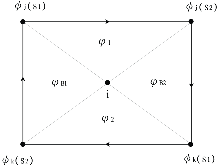
Figure 1: The whole area in the figure corresponds to the off-diagonal geometric phase $\gamma_{jk}$ in Eq. (18). It can be divided into four parts, each corresponding to a phase in Eq. (20), where $\varphi_{B1}=\varphi_{B}(\psi_{j}(s_{1}),\psi_{k}(s_{2}),i)$ and $\varphi_{B2}=\varphi_{B}(\psi_{k}(s_{1}),\psi_{j}(s_{2}),i)$.

References

(1)
M. V.Berry:
Proc. R. Soc. Lond. A, p. 45,
(1984).
(2)
Y. Aharonov and J. Anandan,
Phys. Rev. Lett. 58,
1593 (1987).
(3)
J. Samuel and
R. Bhandari,
Phys. Rev. Lett. 60,
2339 (1988).
(4)
S. Pancharatnam,
Proc. Indian Acad. Sci p. 247
(1956).
(5)
N. Manini and
F. Pistolesi,
Phys. Rev. Lett. 85,
3067 (2000).
(6)
N. Mukunda,
Arvind,
E.Ercolessi,
G.Marmo,
G.Morandi, and
R.Simon,
Phys. Rev. A 67,
042114 (2003).
Filipp and Sjoqvist (2003)
S. Filipp and
E. Sjoqvist,
Phys. Rev. A 68,
042112 (2003).
Hasegawa et al. (2001)
Y. Hasegawa,
R. Loidl,
M. Baron,
G. Badurek, and
H. Rauch,
Phys. Rev. Lett. 87,
070401 (2001).
Hasegawa et al. (2002)
Y. Hasegawa,
R. Loidl,
M. Baron,
N. Manini,
F. Pistolesi,
and H. Rauch,
Phys. Rev. A 65,
052111 (2002).
Nakahara (1990)
M. Nakahara,
Geometry, Topology and Physics
(IOP, 1990).
Shapere and Wilczek (1989)
A. Shapere and
F. Wilczek,
Geometric phases in physics
(World Scientific, 1989).
Wu and Yang (1975)
T. T. Wu and
C. N. Yang,
Phys. Rev. D 12,
3845 (1975).
Bhandari (2002)
R. Bhandari,
Phys. Rev. Lett. 88,
100403 (2002).
Bohm et al. (2003)
A. Bohm,
A. Mostafazadeh,
H. Koizumi,
Q. Niu, and
J. Zwanziger,
The Geometric Phase in Quantum Systems
(Springer, 2003).
Mostafazadeh (1996)
A. Mostafazadeh,
J. Math. Phys. 37,
1218 (1996).
Simon (1983)
B. Simon,
Phys. Rev. Lett. 51,
2167 (1983).
Bhandari (1991)
R. Bhandari,
Phys. Lett. A 157,
221 (1991).
Yuen et al. (2003)
K. W. Yuen,
H. T. Fung,
K. M. Cheng,
M.-C. Chu, and
K. Colanero,
J. Phys. A 36,
11321 (2003).
Simon and Mukunda (1993)
R. Simon and
N. Mukunda,
Phys. Rev. Lett. 70,
880 (1993).