Quantum algorithm to distinguish Boolean functions of different weights

Abstract

By the weight of a Boolean function $f$, denoted by $wt(f)$, we mean the number of inputs for which $f$ outputs $1$. Given a promise that an $n$-variable Boolean function (available in the form of a black box and the output is available in constant time once the input is supplied) is of weight either $wN$ or $(1-w)N$ $(0<w<1,N=2^{n})$, we present a detailed study of quantum algorithms to find out which one actually it is. To solve this problem we apply the Grover’s operator.

First we consider the restricted problem. Given a promise that an $n$-variable Boolean function is of weight either $\lfloor{N\sin^{2}{\frac{k}{2k+1}\frac{\pi}{2}}}\rceil$ or $\lfloor{N\cos^{2}{\frac{k}{2k+1}\frac{\pi}{2}}}\rceil$ ($\lfloor{q}\rceil$ means the nearest integer corresponding to the real value $q$), we show that one can suitably apply Grover’s operator for $k$-many iterations to decide which case this is with a probability almost unity for large $n$ and $k$ in $O(poly(n))$. On the other hand, the best known probabilistic classical algorithm has a success probability close to $0.5$ (from above) after $k$ many steps when $k$ is large. We further show that the best known probabilistic classical algorithm can achieve a success probability almost unity only after $k^{s}$ many iterations where $s>2$. This indicates a quadratic speed up (and also agrees to the quadratic speed up by the use of Grover’s algorithm in database search) on time complexity in the quantum domain with respect to the best known result in the classical domain.

Second, we modify the basic randomized algorithm into a sure success algorithm, which can distinguish Boolean functions of weights $wN$ or $(1-w)N$ for any $w$, $(0<w<1)$. To do that we have exploited a sure success Grover search algorithm, which modifies the very last operation. For the weight decision problem, we show that the very last two operations should be changed to distinguish any weight with certainty and found the phase conditions for the last two operations.

As quantum counting methods exist, which can count the number of solutions, here we compare our method with that. Since the quantum counting method needs to exploit period information, which requires many Grover operations, we have found that our method is faster than the quantum counting method.

Keywords: Quantum Algorithm, Boolean Function, Grover’s Operator, Weight Decision Problem.

1 Introduction

David Deutsch designed a quantum algorithm, which evaluates whether the two outputs of a Boolean function is the same or not using only one function evaluation [5]. Deutsch-Jozsa generalized the Deutsch’s algorithm for more general case such as whether the Boolean function is constant or balanced [6]. Deutsch-Jozsa algorithm had been proposed to show an exponential speed-up in quantum machine than the classical machines. The most important contribution in this area has been achieved when Peter Shor discovered a polynomial-time quantum algorithm for factoring and computing discrete logarithms, which is exponentially faster than the classical best known algorithm [17]. Because this quantum factoring algorithm works in polynomial time compared to exponential time in classical method, many researchers started to find other applications. Lov Grover discovered a quantum database search algorithm, which is quadratic faster than classical database search algorithm [8]. Meanwhile, database search algorithm is one of the most widely used algorithm in the computer applications, the impact is so huge and more researchers are interested in other applications of quantum database search algorithm. This research also focuses on the applications of Grover database search algorithm.

In this research, we assume that there is a promise in the Boolean function as it has a weight $wN$ or $(1-w)N$. Initially, for better understanding, we formulate the problem for some special weight cases such as $\lfloor N\sin^{2}(\frac{k}{2k+1}\frac{\pi}{2})\rceil$ or $\lfloor N\cos^{2}(\frac{k}{2k+1}\frac{\pi}{2})\rceil$, by applying $k$ many Grover operations. Here the quantum algorithm presented is of randomized in nature, but the success probability is arbitrarily close to unity. Next we consider the general case to distinguish functions having weight either $wN$ or $(1-w)N$ and we also consider a deterministic algorithm. This requires changes in the very last two Grover operations with phase conditions. Briefly, from $1^{st}$ to $(k-2)^{th}$ steps, the original Grover operators are used, but, in the last two steps, two different Grover operators are used with the phase conditions. Also we found that the phase conditions depending on the required number of Grover operations. Meanwhile, because quantum counting algorithm was already proposed, we compared two methods. Since the quantum counting method requires more Grover iterations to find period information, we can conclude that our method is faster than this method.

2 Preliminaries

A Boolean function $f(x_{1},\ldots,x_{n})$ on $n$ variables may be viewed as a mapping from $\{0,1\}^{n}$ into $\{0,1\}$. A Boolean function $f$ is constant if $f(x)=c$ for all $x\in\{0,1\}^{n}$, $c\in\{0,1\}$. That means $wt(f)$ is either $0$ or $N$. A Boolean function $f$ is balanced if $wt(f)=N/2$.

Given a promise that the function $f$ is either constant or balanced, one may ask for an algorithm, that can exactly answer which case it is. Note that throughout this document we consider that any Boolean function $f$ is available in the form of an oracle (black box) only, where one can apply an input to the black box to get the output. A classical algorithm needs to check the function for $N/2+1$ inputs in the worst case to decide whether the function is constant or balanced.

Figure 1: Quantum circuit for Deutsch-Jozsa Algorithm

It is known that given a classical circuit for $f$, there is a quantum circuit of comparable efficiency which performs a transformation $U_{f}$ that takes input like $|x,y\rangle$ and produces the output $|x,y\oplus f(x)\rangle$. Given such a $U_{f}$, Deutsch-Jozsa [6] provided a quantum algorithm that can solve this problem in constant time, indeed, in a single evaluation of $U_{f}$. The circuit for their algorithm is given in Fig. 1.

Algorithm 1

Deutsch-Jozsa Algorithm [6]

1.	$|\psi_{0}\rangle=|0\rangle^{\otimes n}|1\rangle$
2.	$|\psi_{1}\rangle=\frac{1}{\sqrt{2N}}\sum_{x\in\{0,1\}^{n}}|x\rangle(|0\rangle-|1\rangle)$
3.	$|\psi_{2}\rangle=\frac{1}{\sqrt{2N}}\sum_{x\in\{0,1\}^{n}}(-1)^{f(x)}|x\rangle(|0\rangle-|1\rangle)$
4.	$|\psi_{3}\rangle=\frac{1}{N\sqrt{2}}\sum_{x,z\in\{0,1\}^{n}}(-1)^{xz\oplus f(x)}|z\rangle(|0\rangle-|1\rangle)$
5.	Measurement at $M$: all-zero state implies that the
	function is constant, otherwise it is balanced.

The Deutsch-Jozsa algorithm yields an exponential speed-up relative to any exact classical computation. This provides a relativized separation between EQP and P with respect to the oracle $f$ (see [16] for basic notions of complexity theory).

Now we discuss a constant time quantum algorithm to distinguish Boolean functions of weight $N/4$ and $3N/4$ [7]. We replace $H^{\otimes n}$ by Grover’s matrix at the output side of $U_{f}$ in Fig. 1 to get a circuit shown in Fig. 2 and show that this solves the problem. In 2001, Green and Pruim [7] presented a relativized separation between BQP and ${\mbox{P}}^{\mbox{NP}}$ using a nice technique based on Grover’s algorithm [8]. Green and Pruim’s work relied on a complexity theoretic formulation, whereas our analysis here is directly related to weights of Boolean functions. Note that a similar question has been discussed in [4, Section 5]. There also the problem was not exactly posed as a discrimination problem, but as a search problem.

We denote the $N\times N$ Grover’s matrix $G_{n}$ as $G_{n}=H^{\otimes n}(2|0\rangle\langle 0|-{\bf{1}})H^{\otimes n}=\frac{2}{N}\sum_{x,y}|x\rangle\langle y|-{\bf{1}}$. It is known that this operation may be constructed with $O(\log N)$ quantum gates [16]. The circuit is shown in Fig. 2 and the steps of the algorithm are as follows.

Figure 2: Quantum circuit to distinguish $wt(f)=N/4$ and $wt(f)=3N/4$

Algorithm 2

Randomized Algorithm to distinguish $wt(f)=3N/4$ or $N/4$

1.	$|\psi_{0}\rangle=|0\rangle^{\otimes n}|1\rangle$
2.	$|\psi_{1}\rangle=\sum_{x\in\{0,1\}^{n}}\frac{|x\rangle}{\sqrt{N}}\frac{(|0\rangle-|1\rangle)}{\sqrt{2}}$
3.	$|\psi_{2}\rangle=\sum_{x\in\{0,1\}^{n}}\frac{(-1)^{f(x)}|x\rangle}{\sqrt{N}}\frac{(|0\rangle-|1\rangle)}{\sqrt{2}}$.
	Let $|\psi^{\prime}_{2}\rangle=\sum_{x\in\{0,1\}^{n}}\frac{(-1)^{f(x)}|x\rangle}{\sqrt{N}}$.
4.	$|\psi_{3}\rangle=G_{n}|\psi^{\prime}_{2}\rangle\frac{(|0\rangle-|1\rangle)}{\sqrt{2}}$
5.	Measure the resulting state $G_{n}|\psi^{\prime}_{2}\rangle$ in the
	computational basis and let the result be ${\hat{x}}$.
6.	if $f({\hat{x}})$ = 0 then $wt(f)=3N/4$ else $wt(f)=N/4$.

The key result proving the correctness of this algorithm is as follows and we present a proof as it will be discussed in details in the following section.

Theorem 1

$G_{n}|\psi^{\prime}_{2}\rangle=\sum_{x:f(x)=0}\frac{N-4\,wt(f)}{N\sqrt{N}}|x\rangle+\sum_{x:f(x)=1}\frac{3N-4\,wt(f)}{N\sqrt{N}}|x\rangle$, and Algorithm 2 produces a correct result.

Proof: $G_{n}|\psi^{\prime}_{2}\rangle\ =\frac{1}{\sqrt{N}}G_{n}\sum_{x\in\{0,1\}^{n}}(-1)^{f(x)}|x\rangle=\frac{1}{\sqrt{N}}\Bigl{(}\frac{4N-2wt(f)}{N}\sum_{x}|x\rangle-\sum_{x}(-1)^{f(x)}|x\rangle\Bigr{)}$. From which the result follows.

If $wt(f)=N/4$ then the probability amplitude of all the $|x\rangle$ for which $f(x)=0$ vanishes. So on measurement we will get some ${\hat{x}}$ for which $f({\hat{x}})$ is 1. On the other hand, if $wt(f)=3N/4$ then the probability amplitude of all the $|x\rangle$ for which $f(x)=1$ vanishes. So on measurement we will get some ${\hat{x}}$ for which $f({\hat{x}})$ is 0.  

3 Repeated Application of Grover’s Operator

Note that Grover’s search algorithm [8] uses repeated applications of $G_{n}$. Motivated by the same idea we now analyze in detail the repeated application of $G_{n}U_{f}$. One may refer the important papers like [2, 3, 4, 9, 10, 11, 12, 13, 14, 15, 18] where the Grover’s operator has been used. We also make an elaborate study to present a comprehensive understanding of this problem in this section. We start with a modification of Algorithm 2.

Algorithm 3

Randomized Algorithm for Weight Decision Problem $3N/4$ and $N/4$

1.	$|\psi_{0}\rangle=|0\rangle^{\otimes n}|1\rangle$
2.	Let us denote $|\psi^{\prime}_{1}\rangle=\sum_{x\in\{0,1\}^{n}}\frac{|x\rangle}{\sqrt{N}}$
3.	$i=0$.
4.	$|\psi_{2}\rangle=U_{f}(|\psi^{\prime}_{1}\rangle\frac{(|0\rangle-|1\rangle)}{\sqrt{2}})$
5.	Let us denote first $n$ qubits of $|\psi_{2}\rangle$ as $|\psi^{\prime}_{2}\rangle$.
6.	$|\psi_{2}\rangle=|\psi^{\prime}_{2}\rangle\frac{(|0\rangle-|1\rangle)}{\sqrt{2}}$.
7.	$|\psi_{3}\rangle=G_{n}|\psi^{\prime}_{2}\rangle\frac{(|0\rangle-|1\rangle)}{\sqrt{2}}$. Let $|\psi_{3}^{\prime}\rangle=G_{n}|\psi^{\prime}_{2}\rangle$.
8.	$i=i+1$.
9.	If $(i<k)$ denote $|\psi^{\prime}_{3}\rangle$ by $|\psi^{\prime}_{1}\rangle$ and go to step 4.
10.	Measure the resulting state $G_{n}|\psi^{\prime}_{2}\rangle$ in the
	computational basis and let the result be ${\hat{x}}$.
11-1.	if $k$ is odd and if $f({\hat{x}})$ = 0 then $wt(f)=\lfloor{N\cos^{2}{\frac{k}{2k+1}\frac{\pi}{2}}}\rceil$
	else $wt(f)=\lfloor{N\sin^{2}{\frac{k}{2k+1}\frac{\pi}{2}}}\rceil$.
11-2.	if $k$ is even and if $f({\hat{x}})=1$ then $wt(f)=\lfloor{N\cos^{2}{\frac{k}{2k+1}\frac{\pi}{2}}}\rceil$
	else $wt(f)=\lfloor{N\sin^{2}{\frac{k}{2k+1}\frac{\pi}{2}}}\rceil$.

In this section we will consider a number of iterations $k\geq 1$ and then show how we can distinguish the weights with a very high (almost unity) success probability. Without loss of generality we detail the analysis by taking odd $k$.

Theorem 2

Let $a_{k}$ denotes the amplitude of the states $|x\rangle$ where $f(x)=0$ and $b_{k}$ denotes the amplitude of the state $|x\rangle$ where $f(x)=1$ after $k$-th iteration. Then, $a_{k}=(2\frac{N-wt(f)}{N}-1)a_{k-1}-2\frac{wt(f)}{N}b_{k-1}$, $b_{k}=2\frac{N-wt(f)}{N}a_{k-1}+(2\frac{N-wt(f)}{N}-1)b_{k-1}$, with initial conditions $a_{0}=b_{0}=\frac{1}{\sqrt{N}}$.

Proof: The proof follows from Algorithm 3 in a similar fashion as the proof of Theorem 1.  

Our interest is to investigate the zeros of $a_{k}$ and $b_{k}$. It may be noted that the solutions to the recurrence relations are given by

$$a_{k}=\frac{1}{\sqrt{N}}\frac{\sin{(2k+1)\beta}}{\sin{\beta}},b_{k}=\frac{1}{\sqrt{N}}\frac{\cos{(2k+1)\beta}}{\cos{\beta}},$$

where $\sin^{2}{\beta}=\frac{wt(f)}{N}$ ($=u$, say for notational convenience). Note that this recursion and Theorem 2 have been described in [4]. Clearly, the factor $1/\sqrt{N}$ does not play any part in determining the zeros of $a_{k}$ and $b_{k}$. The zeros of $a_{k}$ and $b_{k}$ are given by

$$\sin(2k+1)\beta=0,\sin{\beta}\neq 0\ \mbox{ and }\cos(2k+1)\beta=0,\cos{\beta}\neq 0$$

respectively. Now $\sin{(2k+1)\beta}=0\Rightarrow(2k+1)\beta=l\pi\Rightarrow\beta=\frac{l\pi}{(2k+1)}$, where $l\in\mathbb{Z}$. Also $\cos{(2k+1)\beta}=0\Rightarrow(2k+1)\beta=(2m-1)\frac{\pi}{2}\Rightarrow\beta=\frac{(2m-1)}{(2k+1)}\frac{\pi}{2}$ where $m\in\mathbb{Z}$.

As we are interested in distinct roots $u=\sin^{2}{\beta}$ of $a_{k}=0$ (respectively $b_{k}=0$), it is clear that we will get the distinct roots when $1\leq l\leq k$ (respectively $1\leq m\leq k$). We can summarize the above discussion in the following result.

Proposition 3

The $k$ distinct roots of $a_{k}=0$ and $b_{k}=0$ are $\sin^{2}{\frac{l\pi}{(2k+1)}}$ and $\sin^{2}{\frac{(2m-1)}{(2k+1)}\frac{\pi}{2}}$ respectively where $1\leq l,m\leq k$.

Proposition 4

For each root of the equation $a_{k}=0$ there is a corresponding root of the equation $b_{k}=0$ so that their sum is 1.

Proof: The roots of $a_{k}=0$ and $b_{k}=0$ are of the forms $\sin^{2}{\frac{l\pi}{(2k+1)}}$ and $\sin^{2}{\frac{(2m-1)}{(2k+1)}\frac{\pi}{2}}$ respectively where $1\leq l,m\leq k$. Let us consider the pairings of $l,m$ such that $l+m=k+1$. Now $\sin^{2}{\frac{l\pi}{(2k+1)}}+\sin^{2}{\frac{(2m-1)}{(2k+1)}\frac{\pi}{2}}=1$, which gives the proof.  

Given any $k$, Algorithm 3 can distinguish whether a Boolean function is either from the weights $\lfloor{N\sin^{2}{\frac{(2m-1)}{(2k+1)}\frac{\pi}{2}}}\rceil$ or from the weights $\lfloor{N\cos^{2}{\frac{(2m-1)}{(2k+1)}\frac{\pi}{2}}}\rceil$, with good success probability for $m=1,\ldots,k$. However, here we are interested in distinguishing two Boolean functions which are closest in weight to balanced functions, i.e., of weight $\frac{N}{2}=2^{n-1}$.

Definition 1

Let $r_{a,k}$ be the root of $a_{k}=0$ such that $|r_{a,k}-0.5|\leq|\rho_{a,k}-0.5|$ for any root $\rho_{a,k}$ of $a_{k}=0$. Similarly let $r_{b,k}$ be the root of $b_{k}=0$ such that $|r_{b,k}-0.5|\leq|\rho_{b,k}-0.5|$ for any root $\rho_{b,k}$ of $b_{k}=0$. Let us denote $\mu_{k}=\min\{r_{a,k},r_{b,k}\}$.

Proposition 5

$$\mu_{k} = r_{a,k}=\sin^{2}{\frac{2\alpha-1}{4\alpha-1}\frac{\pi}{2}},\mbox{ when }k=2\alpha-1\mbox{ and }m=\alpha$$

$$= r_{b,k}=\sin^{2}{\frac{2\alpha}{4\alpha+1}\frac{\pi}{2}},\mbox{ when }k=2\alpha\mbox{ and }l=\alpha.$$

Proof: Let $k=2\alpha-1$. For $m=\alpha$, the root of $a_{k}=0$ is $\rho_{a,k}=\sin^{2}{\frac{2\alpha-1}{4\alpha-1}\frac{\pi}{2}}$. For $m=\alpha+1$, the root of $a_{k}=0$ is $\rho^{\prime}_{a,k}=\sin^{2}{\frac{2\alpha+1}{4\alpha-1}\frac{\pi}{2}}$. As $2\alpha+1>2\alpha$, $\sin^{2}{\frac{2\alpha+1}{4\alpha-1}\frac{\pi}{2}}>\sin^{2}{\frac{2\alpha}{4\alpha-1}\frac{\pi}{2}}$, which gives, $\sin^{2}{\frac{2\alpha+1}{4\alpha-1}\frac{\pi}{2}}+\cos^{2}{\frac{2\alpha}{4\alpha-1}\frac{\pi}{2}}>1$, i.e., $\sin^{2}{\frac{2\alpha+1}{4\alpha-1}\frac{\pi}{2}}+\sin^{2}{\frac{2\alpha-1}{4\alpha-1}\frac{\pi}{2}}>1$, i.e., $\sin^{2}{\frac{2\alpha+1}{4\alpha-1}\frac{\pi}{2}}-\frac{1}{2}>\frac{1}{2}-\sin^{2}{\frac{2\alpha-1}{4\alpha-1}\frac{\pi}{2}}$ which gives $\rho^{\prime}_{a,k}-\frac{1}{2}>\frac{1}{2}-\rho_{a,k}$. Since all the other roots of $a_{k}=0$ are either less than $\rho_{a,k}$ or greater than $\rho^{\prime}_{a,k}$, we get $r_{a,k}=\rho_{a,k}$. It is also clear that $r_{b,k}=1-r_{a,k}$ and hence here $r_{b,k}>r_{a,k}$. So $\mu_{k}=r_{a,k}$.

Let $k=2\alpha$. For $m=\alpha$, the root of $b_{k}=0$ is $\rho_{b,k}=\sin^{2}{\frac{2\alpha}{4\alpha+1}\frac{\pi}{2}}$. For $m=\alpha+1$, the root of $b_{k}=0$ is $\rho^{\prime}_{a,k}=\sin^{2}{\frac{2\alpha+2}{4\alpha+1}\frac{\pi}{2}}$. As $2\alpha+2>2\alpha+1$, $\sin^{2}{\frac{2\alpha+2}{4\alpha+1}\frac{\pi}{2}}>\sin^{2}{\frac{2\alpha+1}{4\alpha+1}\frac{\pi}{2}}$, which gives, $\sin^{2}{\frac{2\alpha+2}{4\alpha+1}\frac{\pi}{2}}+\cos^{2}{\frac{2\alpha+1}{4\alpha+1}\frac{\pi}{2}}>1$, i.e., $\sin^{2}{\frac{2\alpha+2}{4\alpha+1}\frac{\pi}{2}}+\sin^{2}{\frac{2\alpha}{4\alpha+1}\frac{\pi}{2}}>1$, i.e., $\sin^{2}{\frac{2\alpha+2}{4\alpha+1}\frac{\pi}{2}}-\frac{1}{2}>\frac{1}{2}-\sin^{2}{\frac{2\alpha}{4\alpha+1}\frac{\pi}{2}}$ which gives $\rho^{\prime}_{b,k}-\frac{1}{2}>\frac{1}{2}-\rho_{b,k}$. Since all the other roots of $b_{k}=0$ are either less than $\rho_{b,k}$ or greater than $\rho^{\prime}_{b,k}$, we get $r_{b,k}=\rho_{b,k}$. It is also clear that $r_{a,k}=1-r_{b,k}$ and hence here $r_{a,k}>r_{b,k}$. So $\mu_{k}=r_{b,k}$.  

Theorem 6

$\mu_{k}=\sin^{2}{\frac{k}{2k+1}\frac{\pi}{2}}$ and $\mu_{k}<\mu_{k+1}<0.5$.

Proof: From Proposition 5, it is clear that $\mu_{k}=\sin^{2}{\frac{k}{2k+1}\frac{\pi}{2}}$. So $\mu_{k+1}=\sin^{2}{\frac{k+1}{2k+3}\frac{\pi}{2}}$. Now $\frac{k+1}{2k+3}-\frac{k}{2k+1}=\frac{1}{(2k+3)(2k+1)}>0$, which gives $\mu_{k+1}>\mu_{k}$. Further it is easy to see that $\mu_{k+1}=\sin^{2}{\frac{k+1}{2k+3}\frac{\pi}{2}}<\sin^{2}{\frac{\pi}{4}}<\frac{1}{2}$.  

As $a_{k}$ and $b_{k}$ can be seen as polynomials in $u$, we now refer them as $a_{k}(u)$ and $b_{k}(u)$, respectively. It is clear that $a_{k}(\mu_{k})=0$. Now using Algorithm 3, we can distinguish two Boolean functions of weight $\mu_{k}N$ and $(1-\mu_{k})N$. Unfortunately, $\mu_{k}N$ may not be an integer and in that case we have to consider a Boolean function of weight $\mu_{k}^{\prime}N$, where $\mu_{k}^{\prime}N$ is an integer and $|\mu_{k}^{\prime}N-\mu_{k}N|\leq 0.5$. Thus we will be using the Algorithm 3 to distinguish between Boolean functions of weight $\mu_{k}^{\prime}N$ and $(1-\mu_{k}^{\prime})N$. This will incorporate some error in the decision process. However, we will show that this error is almost zero for large $N$.

Theorem 7

Consider Boolean functions on $n$ variables and let $N=2^{n}$. After $k$ iterations, $k$ in $O(poly(n))$, the quantum algorithm (Algorithm 3) can distinguish two Boolean functions of weights $\lfloor{N\sin^{2}{\frac{k}{2k+1}\frac{\pi}{2}}}\rceil$ and $\lfloor{N\cos^{2}{\frac{k}{2k+1}\frac{\pi}{2}}}\rceil$ with success probability $>1-\frac{64(k+1)^{2}}{N^{2}}$ which is almost unity for large $N$.

Proof: We have $a_{k}=\frac{1}{\sqrt{N}}\frac{\sin{(2k+1)\beta}}{\sin{\beta}}=0$, when $\sin^{2}{\beta}=\mu_{k}$. Let $\mu_{k}^{\prime}=\sin^{2}{\beta^{\prime}}$. We like to calculate the value of $a_{k}(\mu_{k}^{\prime})=\frac{1}{\sqrt{N}}\frac{\sin{(2k+1)\beta^{\prime}}}{\sin{\beta^{\prime}}}$.

As $|\mu_{k}^{\prime}N-\mu_{k}N|\leq 0.5$, we get $|\sin^{2}{\beta^{\prime}}-\sin^{2}{\beta}|\leq\frac{0.5}{N}$. Thus $(\sin{\beta^{\prime}}+\sin{\beta})|\sin{\beta^{\prime}}-\sin{\beta}|\leq\frac{0.5}{N}$, i.e., $(2\sin{\frac{\beta^{\prime}+\beta}{2}}\cos{\frac{\beta^{\prime}-\beta}{2}})(2\cos{\frac{\beta^{\prime}+\beta}{2}}|\sin{\frac{\beta^{\prime}-\beta}{2}}|)\leq\frac{0.5}{N}$, i.e., $(2\sin{\frac{\beta^{\prime}+\beta}{2}}\cos{\frac{\beta^{\prime}+\beta}{2}})(2\cos{\frac{\beta^{\prime}-\beta}{2}}|\sin{\frac{\beta^{\prime}-\beta}{2}}|)\leq\frac{0.5}{N}$, i.e., $\sin{(\beta^{\prime}+\beta)}|\sin{(\beta^{\prime}-\beta)}|\leq\frac{0.5}{N}$. This implies, $|\sin{(\beta^{\prime}-\beta)}|\leq\frac{1}{2N\sin{(\beta^{\prime}+\beta)}}$. Note that $\frac{1}{4}=\mu_{1}<\mu_{k}<\frac{1}{2}$ for $k>1$. Now $\mu_{k}=\sin^{2}{\beta}$. So, $\frac{\pi}{6}<\beta<\frac{\pi}{4}$. As $\beta\approx\beta^{\prime}$, $\beta+\beta^{\prime}\approx 2\beta$. Due to the small difference between $\beta$ and $\beta^{\prime}$, it may happen that on the lower side $\beta+\beta^{\prime}$ may marginally be less than $2\frac{\pi}{6}$ and at the higher side may marginally exceed $2\frac{\pi}{4}$. Thus it is safe to assume $\sin{(\beta+\beta^{\prime})}>\frac{1}{2}$. Hence $|\sin{(\beta^{\prime}-\beta)}|<\frac{1}{2N\frac{1}{2}}=\frac{1}{N}$. Since $|\frac{\beta^{\prime}-\beta}{2}|<|\sin{(\beta^{\prime}-\beta)}|<|\beta^{\prime}-\beta|$, we can write $|\frac{\beta^{\prime}-\beta}{2}|<\frac{1}{N}$, i.e., $|\beta^{\prime}-\beta|<\frac{2}{N}$.

One can take $\phi(\beta)=\frac{\sin{(2k+1)\beta}}{\sin{\beta}}$ and use Taylor’s series expansion for $\phi(\beta)$ to get the upper bound on $|\frac{\sin{(2k+1)\beta^{\prime}}}{\sin{\beta^{\prime}}}-\frac{\sin{(2k+1)\beta}}{\sin{\beta}}|$. We consider $\phi(\beta+h)=\frac{\sin{(2k+1)\beta^{\prime}}}{\sin{\beta^{\prime}}}$, where $h=\beta^{\prime}-\beta$ is a small quantity. Now $\phi(\beta+h)-\phi(\beta)\approx h\frac{d\phi(\beta)}{d\beta}$ with error term bounded by $R_{1}(\beta)$, the remainder when only the first term in the Taylor’s series is considered. As $k$ increases, the value of $\beta$ falls in the neighbourhood of $\frac{\pi}{4}$. It can be checked that $|\frac{d\phi(\beta)}{d\beta}|_{\beta=\frac{\pi}{4}}<\sqrt{2}(2k+2)$. Also we calculate $|R_{1}(\frac{\pi}{4})|=\frac{h^{2}}{2}|\frac{d^{2}\phi(\beta)}{d\beta^{2}}|_{\beta=\frac{\pi}{4}+\alpha h}<\frac{h^{2}}{2}\sqrt{2((2k+1)^{2}-1)^{2}+16}$, where $0<\alpha<1$. As $|\phi(\beta+h)-\phi(\beta)|<|\frac{d\phi(\beta)}{d\beta}|_{\beta=\frac{\pi}{4}}+|R_{1}(\frac{\pi}{4})|$, we get $|\frac{\sin{(2k+1)\beta^{\prime}}}{\sin{\beta^{\prime}}}-\frac{\sin{(2k+1)\beta}}{\sin{\beta}}|<\frac{8(k+1)}{N}$.

Since, $\frac{\sin{(2k+1)\beta}}{\sin{\beta}}=0$, we have $\frac{\sin{(2k+1)\beta^{\prime}}}{\sin{\beta^{\prime}}}<\frac{8(k+1)}{N}$. Thus $a_{k}(\mu_{k}^{\prime})=\frac{1}{\sqrt{N}}\frac{\sin{(2k+1)\beta^{\prime}}}{\sin{\beta^{\prime}}}<\frac{8(k+1)}{N\sqrt{N}}$.

Thus, if $wt(f)=\mu_{k}N$, then we would have got $x$ such that $f(x)=1$ with certainty. As $\mu_{t}N$, may not be an integer, we have considered functions with $wt(f)=\mu_{k}^{\prime}N$ which is an integer such that $|\mu_{k}^{\prime}N-\mu_{k}N|\leq 0.5$. In this case the probability of (wrongly) observing an $x$ such that $f(x)=0$ is $(a_{k}(\mu_{k}^{\prime}))^{2}(1-\mu_{k}^{\prime})N<(\frac{8(k+1)}{N\sqrt{N}})^{2}(1-\mu_{k}^{\prime})N<\frac{64(k+1)^{2}}{N^{2}}$.

Similarly, if $wt(f)=(1-\mu_{k})N$, then we would have got $x$ such that $f(x)=0$ with certainty. As $(1-\mu_{k})N$, may not be an integer, we have to consider functions with $wt(f)=(1-\mu_{k}^{\prime})N$ which is an integer. In this case the probability of (wrongly) observing an $x$ such that $f(x)=1$ is $<\frac{64(k+1)^{2}}{N^{2}}$.  

Since the function $f$ is available in the form of an oracle, the best known classical probabilistic algorithm can work as follows. For $k$ many iterations it can present random inputs to the oracle and guess the function is of lower weight if the output zero appears more frequently and guess the function is of higher weight if the output one appears more frequently. As we consider the majority rule, we choose the number of iterations as odd in the classical probabilistic algorithm. This will always guarantee majority of either output zero or output one (in the case of an even number of iterations there may be the possibility of a tie and then a random decision has to be taken). For general analysis, the estimate of probabilities will remain almost the same, and we only present the analysis when the number of iterations is odd.

Note that for classical lower bound proofs to determine the majority one may refer to [1]. However, we provide a complete result with proof which is suitable for our analysis. Here, the probability of the correct answer in a single step is $\cos^{2}{\frac{k}{2k+1}\frac{\pi}{2}}$. After $g(k)$ many iterations, $g(k)$ in $\Omega(k)$, probability of success $p_{s}=1-\sum_{i=0}^{\frac{g(k)-1}{2}}\mbox{$\left({g(k)\atop i}\right)$}(\cos^{2}{\frac{\pi k}{2(2k+1)}})^{i}(\sin^{2}{\frac{\pi k}{2(2k+1)}})^{g(k)-i}$. Let us now present the following technical result.

Proposition 8

For odd positive integer $k$ and $g(k)$ be in $\Omega(k)$, let

$$E(k,g(k))=\sum_{i=0}^{\frac{g(k)-1}{2}}\mbox{$\left({g(k)\atop i}\right)$}(\cos^{2}{\frac{\pi k}{2(2k+1)}})^{i}(\sin^{2}{\frac{\pi k}{2(2k+1)}})^{g(k)-i}.$$

Then

$\lim_{k\rightarrow\infty}E(k,k)$	$=$	$0.5$,
$\lim_{k\rightarrow\infty}E(k,k^{2})$	$>$	$0.2$ and
$\lim_{k\rightarrow\infty}E(k,k^{s})$	$=$	$0$ for $s>2$.

Proof: Let $X_{k}$ follow an identical and independent binomial distribution having the parameters $g(k),p_{k}=\cos^{2}{\frac{\pi k}{2(2k+1)}}$. Let $\eta_{k}=E(k,g(k))=\sum_{i=0}^{\frac{g(k)-1}{2}}\mbox{$\left({g(k)\atop i}\right)$}(p_{k})^{i}(1-p_{k})^{g(k)-i}=Prob(X_{k}\leq\frac{g(k)-1}{2})$. Consider $X_{k,i}\sim iid\ Bernoulli(p_{k})$, where $1\leq i\leq g(k)$. So, $X_{k}=X_{k,1}+\ldots+X_{k,g(k)}$. Thus, $var(X_{k})=\sigma_{k}^{2}=var(X_{k,1}+\ldots+X_{k,g(k)})=g(k)p_{k}(1-p_{k})$.

Since $g(k)\rightarrow\infty$ as $k\rightarrow\infty$, the Central Limit Theorem is applicable. Define $Z_{k}=\frac{X_{k}-g(k)p(k)}{\sigma_{k}}$. So $\eta_{k}=Prob(X_{k}\leq\frac{g(k)-1}{2})=Prob(Z_{k}\leq\zeta_{k})$, where $\zeta_{k}=\frac{g(k)(\frac{1}{2}-p_{k})-\frac{1}{2}}{\sigma_{k}}$. Suppose, $\lim_{k\rightarrow\infty}\zeta_{k}=\zeta\in\mathbb{R}$. Since convergence in distribution holds in this case, $\lim_{k\rightarrow\infty}\eta_{k}=\Phi(\zeta)$, where $\Phi$ is the cumulative distribution function of the standard normal variate. Hence, $\zeta=\lim_{k\rightarrow\infty}\zeta_{k}=\lim_{k\rightarrow\infty}\frac{g(k)(\frac{1}{2}-p_{k})-\frac{1}{2}}{\sigma_{k}}=\lim_{k\rightarrow\infty}\frac{g(k)(\frac{1}{2}-p_{k})-\frac{1}{2}}{\sqrt{g(k)p_{k}(1-p_{k})}}=\lim_{k\rightarrow\infty}\sqrt{g(k)}(1-2p_{k})$ as $\lim_{k\rightarrow\infty}\sqrt{p_{k}(1-p_{k})}=\frac{1}{2}$. Thus,

$\zeta$	$=$	$\lim_{k\rightarrow\infty}\sqrt{g(k)}(-\cos{\frac{\pi k}{2k+1}})$
	$=$	$-\lim_{k\rightarrow\infty}\sqrt{g(k)}\sin{\frac{\pi}{4k+2}}$
	$=$	$-\lim_{k\rightarrow\infty}\frac{\sin{\frac{\pi}{4k+2}}}{\frac{\pi}{4k+2}}\frac{\pi}{4k+2}\sqrt{g(k)}$
	$=$	$-\lim_{k\rightarrow\infty}\frac{\pi}{4k+2}\sqrt{g(k)}$.

So we get, $\zeta=0$ when $g(k)=t$, $\zeta=-\frac{\pi}{4}$ when $g(k)=k^{2}$ and $\zeta=-\infty$, when $g(k)=k^{s},s>2$. Hence, $\lim_{k\rightarrow\infty}\eta_{k}$ is $=\Phi(0)=0.5$, when $g(k)=k$, $=\Phi(-\frac{\pi}{4})>0.2$ when $g(k)=k^{2}$ and $=\Phi(-\infty)=0$ when $g(k)=k^{s},s>2$. This gives the proof.  

Theorem 9

Consider Boolean functions on $n$ variables and let $N=2^{n}$. After $k$ iterations, the best known classical probabilistic algorithm can distinguish two Boolean functions of weights $\lfloor{N\sin^{2}{\frac{k}{2k+1}\frac{\pi}{2}}}\rceil$ and $\lfloor{N\cos^{2}{\frac{k}{2k+1}\frac{\pi}{2}}}\rceil$ with success probability $p_{s}=0.5$ when $g(k)=k$, $p_{s}<0.8$ when $g(k)=k^{2}$ and $p_{s}=1$ when $g(k)=k^{s},s>2$, for large $k$.

Proof: The proof follows from $p_{s}=1-\sum_{i=0}^{\frac{g(k)-1}{2}}\mbox{$\left({g(k)\atop i}\right)$}(\cos^{2}{\frac{\pi k}{2(2k+1)}})^{i}(\sin^{2}{\frac{\pi k}{2(2k+1)}})^{g(k)-i}$ and the results in Proposition 8.  

Based on the results of Theorem 7 and Theorem 9, it is clear that when the quantum algorithm can achieve a success probability almost unity, then the best known classical algorithm can achieve a success probability almost $0.5$ (from above) after $k$ many steps. The classical algorithm can achieve a success probability almost unity only after $k^{s}$ many steps for $s>2$. Thus the quantum algorithm can achieve a quadratic speed up in this case.

3.1 Distinguishing Boolean functions from two different Sets of Weights

$k$	The roots of $a_{k}=0$ (top line) and $b_{k}=0$ (bottom line)
1	0.250000,
	0.750000,
2	0.095492, 0.654508,
	0.345492, 0.904508,
3	0.049516, 0.388740, 0.811745,
	0.188255, 0.611260, 0.950484,
4	0.030154, 0.250000, 0.586824, 0.883022,
	0.116978, 0.413176, 0.750000, 0.969846,
5	0.020254, 0.172570, 0.428843, 0.707708, 0.920627,
	0.079373, 0.292292, 0.571157, 0.827430, 0.979746,
6	0.014529, 0.125745, 0.322698, 0.560268, 0.784032, 0.942728,
	0.057272, 0.215968, 0.439732, 0.677302, 0.874255, 0.985471,
7	0.010926, 0.095492, 0.250000, 0.447736, 0.654508, 0.834565, 0.956773,
	0.043227, 0.165435, 0.345492, 0.552264, 0.750000, 0.904508, 0.989074,
8	0.008513, 0.074891, 0.198683, 0.363169, 0.546134, 0.722869, 0.869504, 0.966236,
	0.033764, 0.130496, 0.277131, 0.453866, 0.636831, 0.801317, 0.925109, 0.991487,
9	0.006819, 0.060263, 0.161359, 0.299152, 0.458710, 0.622743, 0.773474, 0.894570, 0.972909,
	0.027091, 0.105430, 0.226526, 0.377257, 0.541290, 0.700848, 0.838641, 0.939737, 0.993181,
10	0.005585, 0.049516, 0.133474, 0.250000, 0.388740, 0.537365, 0.682671, 0.811745, 0.913119, 0.977786,
	0.022214, 0.086881, 0.188255, 0.317329, 0.462635, 0.611260, 0.750000, 0.866526, 0.950484, 0.994415,

Table 1: Roots of $a_{k}=0$ and $b_{k}=0$.

Let us consider two different sets $A_{k}$ and $B_{k}$, where $A_{k}$ contains the roots of $a_{k}=0$ and $B_{k}$ contains the roots of $b_{k}=0$. From Proposition 3, it is clear that $A_{k}=\{\sin^{2}{\frac{(2m-1)}{(2k+1)}\frac{\pi}{2}}|m=1,\ldots,k\}$ and $B_{k}=\{\cos^{2}{\frac{(2m-1)}{(2k+1)}\frac{\pi}{2}}|m=1,\ldots,k\}$. One can see Table 1 for a few examples.

Given any $k$, Algorithm 3 can distinguish whether a Boolean function is either from the weights $\lfloor N\sin^{2}{\frac{(2m-1)}{(2k+1)}\frac{\pi}{2}}\rceil$ or from the weights $\lfloor N\cos^{2}{\frac{(2m-1)}{(2k+1)}\frac{\pi}{2}}\rceil$, with good success probability for $m=1,\ldots,k$. This also helps in solving the question can we distinguish two Boolean functions of weights $Nw_{1}$ and $Nw_{2}$ where $w_{1}+w_{2}\neq 1$? As example, one can check the case for $k=10$ in Table 1, where we may be able to distinguish Boolean functions with weights $Nw_{1}$ and $Nw_{2}$, for $w_{1}\approx 0.388740$ and $w_{2}\approx 0.317329$. However, we leave this for future research as in this paper we mainly focus on distinguishing functions having weights $Nw$ and $N(1-w)$.

4 Sure Success Weight Decision Algorithm

4.1 Motivation

By Theorem 7, we know that the Algorithm 3 is a randomized one and not sure success algorithm. In the Grover-like database search algorithms, number of ideas have been proposed to achieve sure success. We try to exploit similar strategies here, though we need to make certain subtle modifications for this purpose.

4.2 Brassard’s Sure Success Database Search

Many algorithms have been proposed for a sure success database search algorithm based on Grover search [11, 10, 18, 9, 13, 2]. Meanwhile, we need to reformulate and to generalize the original Grover operators, $G_{n}$ and $U_{f}$, for a sure success method as follows.

$G_{n}=-I_{|\psi_{0}\rangle}(\theta)=-\{I-(1-e^{i\theta})|\psi_{0}\rangle\langle\psi_{0}|\}$.

$U_{f}=I_{|solution\rangle}(\phi)=I-(1-e^{i\phi})|solution\rangle\langle solution|$.

A sure success database search can find one of solutions exactly by changing two phases, $\theta$ and $\phi$ of $I_{|\psi_{0}\rangle}(\theta)$ and $I_{|solution\rangle}(\phi)$. Can we apply this kind sure success approach in the Grover database search into our problem? We try to exploit Brassard method [2] for this. The method is based on the following approach. The required minimum number of Grover operation is calculated, which assumes to be $k$. Then, from $1^{st}$ to ${(k-1)}^{th}$ operation, the original Grover operation is applied. However, for the last $k^{th}$ operation, a slightly different Grover operation is applied by controlling two phases, $\theta$ and $\phi$ for $I_{|\psi_{0}\rangle}(\theta)$ and $I_{|solution\rangle}(\phi)$. Figures 3(a) and 3(b) show the Brassard’s method in the Hilbert space and Bloch sphere, respectively. Please note that the inversion operators, $-I_{|\psi_{0}\rangle}(\theta)I_{|solution\rangle}(\phi)$ in the Hilbert space, correspond to the rotation operators, $-e^{i(\frac{\theta}{2}+\frac{\phi}{2})}R_{|\psi_{0}\rangle}(-\theta)R_{|solution\rangle}(-\phi)$ in the Bloch sphere [12]. As shown in the figures, the last step of the Grover operation uses different phases for two inversions in the Hilbert space and for two rotations in the Bloch Sphere.

(a) Hilbert Space

(b) Bloch Sphere

Figure 3: Brassard’s Sure Success Database Search

4.3 Approach

At the first sight, it looks that Brassard method can be directly applied for the weight decision problem. However, it is a little bit different from the Brassard’s case. Brassard method changes only the last step because the goal of this approach is to rotate the $(k-1)^{th}$ state to the solution state. However, in the weight decision case, we need to satisfy that two initial states for different weights should be rotated to the solution and the non-solution state exclusively after operations. In other words, if the proposed method rotates the initial state for $wN$ weight case to the solution state, the same operation should rotate the initial state for $(1-w)N$ weight case to the non-solution state. By this condition, we can make a relation between the initial states for $wN$ and $(1-w)N$ to the solution and non-solution states. Finally, we can decide the weight exactly from measuring the final state and evaluating the function with the measured value $\hat{x}$. To satisfy this condition, we proposed a method which changes the very last two operations. As a result, from $1^{st}$ to ${(k-2)}^{th}$ operation, we use the ($\pi$,$\pi$) phase angles for the $I_{|\psi_{0}\rangle}(\theta)$ and $I_{|solution\rangle}(\phi)$ operations. However, for ${(k-1)}^{th}$ and $k^{th}$ operation, ($-\theta_{1}$, $\pi$) and ($-\theta_{2}$, $\pi$) phases should be used, respectively. Algorithm 4 describes the overall idea.

Algorithm 4

Sure Success Weight Decision Algorithm

1.	$|\psi_{0}\rangle=|0\rangle^{\otimes n}|1\rangle$, $i=0$,
	if $0<Nmin(w,1-w)\leq Nsin^{2}\frac{\pi}{5}$, $k$ is 2,
	otherwise, $k$ satisfies $Nsin^{2}{\frac{k-1}{2k-1}\frac{\pi}{2}}<Nmin(w,1-w)\leq Nsin^{2}{\frac{k}{2k+1}\frac{\pi}{2}}$.
	$\frac{k-1}{2k-1}\pi<\beta_{for\,smaller\,weight}\leq\frac{k}{2k+1}\pi$.
	$\pi-\frac{k-1}{2k-1}\pi>\beta_{for\,bigger\,weight}\geq\pi-\frac{k}{2k+1}\pi$.
2.	while($i<(k-2)$) do
	{
	$|\psi_{i+1}\rangle=-I_{|\psi_{0}\rangle}(\pi)I_{|solution\rangle}(\pi)|\psi_{i}\rangle$
	$i=i+1$
	}
3.	$|\psi_{k-1}\rangle=-I_{|\psi_{0}\rangle}(-\theta_{1})I_{|solution\rangle}(\pi)|\psi_{k-2}\rangle$
4.	$|\psi_{k}\rangle=-I_{|\psi_{0}\rangle}(-\theta_{2})I_{|solution\rangle}(\pi)|\psi_{k-1}\rangle$
5.	measure $|\psi_{k}\rangle$ in the computational basis.
	let the result be ${\hat{x}}$.
6-1.	if $k$ is odd and if $f({\hat{x}})$ = 0 then
	$wt(f)=Nmax(w,1-w)$
	else $wt(f)=Nmin(w,1-w)$.
6-2.	if $k$ is even and if $f({\hat{x}})$ = 1 then
	$wt(f)=Nmax(w,1-w)$
	else $wt(f)=Nmin(w,1-w)$.

4.4 Alternative Final State

In the Brassard database search algorithm, the final state should be the solution state. However, in the weight distinction case, two final states after $k$ operations should be located in the solution and non-solution state exclusively. Meanwhile, there are no restrictions of the locations of final states except that two final states should be located at solution and non-solution states exclusively. Hence the locations of two final states can be alternatively changed with the required number of operations. As a result, we need to think about the final states of the proposed method. The previously proposed method, Algorithm 3, is a special case where the ($\pi$, $\pi$) phase angles are used for the $I_{|\psi_{0}\rangle}(\theta)$ and $I_{|solution\rangle}(\phi)$ operations. Hence we can infer that the final state for the smaller weight case after $k$ operations in the special weight decision algorithm, in Bloch sphere, is

$$\left({{\begin{array}[]{*{20}c}{\sin(2k+1)\beta\hfill}\\ 0\hfill\\ {-\cos(2k+1)\beta\hfill}\\ \end{array}}}\right),$$ (1)

where $\beta=\frac{k}{2k+1}\pi$. Note that all state vectors are represented in the Bloch sphere hereafter. Therefore, we can know that the final state for the smaller wight is alternatively changed with the required $k$ operations such as

$$\left({{\begin{array}[]{*{20}c}{\sin((2k+1)\frac{k}{2k+1}\pi)\hfill}\\ 0\hfill\\ {-\cos((2k+1)\frac{k}{2k+1}\pi)\hfill}\\ \end{array}}}\right)=\left({{\begin{array}[]{*{20}c}{\sin(k\pi)\hfill}\\ 0\hfill\\ {-\cos(k\pi)\hfill}\\ \end{array}}}\right)=\left\{{\begin{array}[]{l}\left({{\begin{array}[]{*{20}c}0\hfill\\ 0\hfill\\ {+1\hfill}\\ \end{array}}}\right)$for odd$\,k\\ \left({{\begin{array}[]{*{20}c}0\hfill\\ 0\hfill\\ {-1\hfill}\\ \end{array}}}\right)$for even$\,k\\ \end{array}}\right..$$ (2)

Meanwhile, the $(0,0,+1)^{t}$ and $(0,0,-1)^{t}$ states in Bloch sphere represent solution and non-solution states in Hilbert space, respectively. In summary, if the required number of $k$ is odd, the final state for the smaller (bigger) weight case should be located in the solution (non-solution) state. On the other hand, if the required number of $k$ is even, the final state for the smaller (bigger) weight case should be located in the non-solution (solution) state. On the other hand, for the bigger weight case, we can easily analyze the alternative final state based on the number of operations with the initial angle, $\pi-\beta$. This analysis means that we need to find two phase conditions with the required number of operations.

4.5 Modification of Last Two Operations

Figure 4 explains how we can rotate two initial states to different final states, which should be located in the different poles in Bloch sphere as solution,$(0,0,+1)^{t}$, and non-solution,$(0,0,-1)^{t}$, state. Note that Figure 4 shows the case when only two operations are sufficient to decide the exact weight. In the figure, the circle and diamond mean two states, which have the smaller and the bigger weight, respectively. Our purpose is to find phase conditions, which can rotate two initial states to different poles exclusively with the same phase conditions. Hence if the weight is the smaller (bigger) one and the method rotates the initial state to the solution state, the method should rotate the initial state of the bigger (smaller) weight case to the non-solution state. Note that all figures hereafter are viewed from $+Y$ direction in the Bloch sphere for easy understanding. Therefore, only $X$ and $Z$ directions and the $X-Z$ plane are shown in all the figures. In the initial step, two initial states $|A_{0}\rangle$ and $|B_{0}\rangle$ are $(\sin\beta,0,-\cos\beta)^{t}$ and $(\sin(\pi-\beta),0,-\cos(\pi-\beta))^{t}=(\sin\beta,0,\cos\beta)^{t}$, respectively. At the first step, two initial states are rotated to $|A_{1}\rangle$ and $|B_{1}\rangle$ states by using rotation $R_{|solution\rangle}(\pi)$. Therefore, only the sign of $x$ is changed. In the second step, two last states are rotated to $|A_{2}\rangle$ and $|B_{2}\rangle$ states by using rotation $R_{|\psi_{0}\rangle}(\theta_{1})$. Meanwhile, $|A_{1}\rangle$ state should be rotated to $|A_{2}\rangle$ state, which is the cross point between line $A1$ and line $f$. The line $f$ is a path, where the point $|A_{1}\rangle$ can be rotated by the rotation $R_{|\psi_{0}\rangle}(\theta_{1})$. As the same rule, the same rotation operator rotates $|B_{1}\rangle$ state to $|B_{2}\rangle$ state, where $|B_{2}\rangle$ state is the cross point between line $B1$ and line $1-f$. Because two last states are rotated with the same phase angle, the value of $x$ is the same, but values of $y$ and $z$ have different sign values between them. At the third step, $R_{|solution\rangle}(\pi)$ operator is used for the last two states. Therefore, the signs of $x$ and $y$ are changed as shown in $|A_{3}\rangle$ and $|B_{3}\rangle$ states. At the last step, the two final states are rotated to two different poles exclusively by using the same rotation angle, $\theta_{2}$. In other words, $|A_{3}\rangle$ state moves to the $-Z$ pole, non-solution state, and $|B_{3}\rangle$ to the $+Z$ pole, solution state. Finally, if we measure the final state and the measured value, then $\hat{x}$, is one of solutions (non-solutions) and we can decide that the weight is bigger (smaller) one. Meanwhile, the key point of this approach is to find two cross points, $|A_{2}\rangle$ and $|B_{2}\rangle$ with the required number of operations.

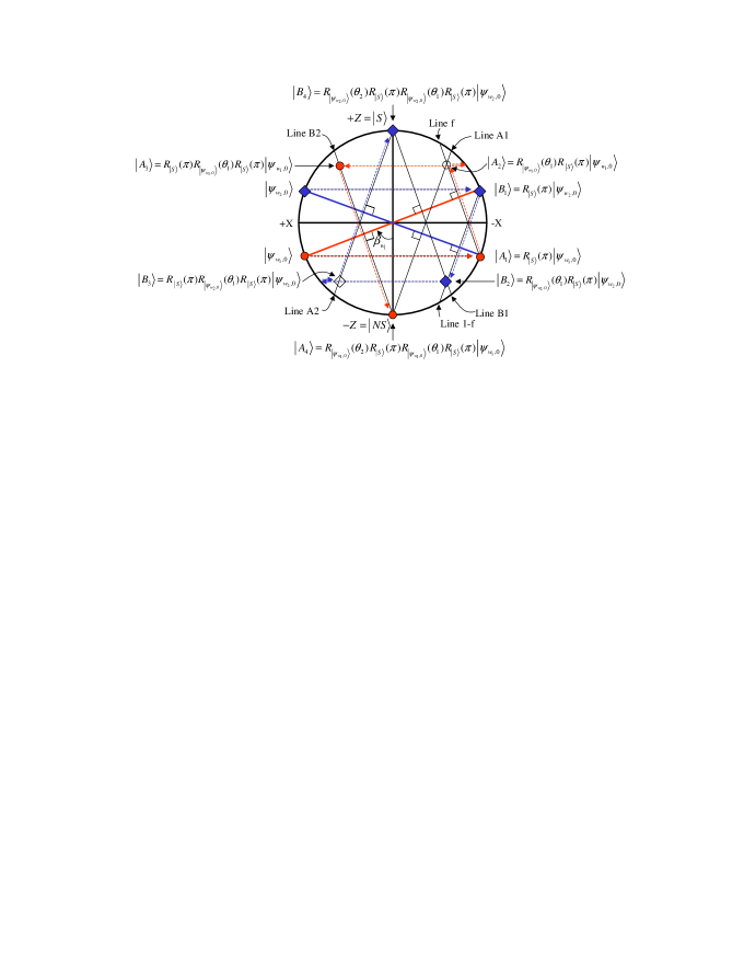
Figure 4: Last Two Operations

4.6 Correctness

In the proposed method, we have to change two phases only for the last two operations, not for other operations because until $(k-2)^{th}$ operation, there is no cross point such as $|A_{2}\rangle$ and $|B_{2}\rangle$ in Figure 4. Therefore, we need to show that until $(k-2)^{th}$ operation, there are no cross point, but in the $(k-1)^{th}$ operation, there are two cross points. For easy explanation, we only consider when the required number of operation is odd case and the weight is smaller one. Hence $k$ is odd and $\frac{k-1}{2k-1}\pi<\beta\leq\frac{k}{2k+1}\pi$. Other cases can be proved with the same approach.

4.6.1 No Cross Point until $(k-2)^{th}$ Operation

Figure 5(a) shows the last state, $|\psi_{k-2}\rangle$, when $(k-2)$ operations of $R_{|\psi_{0}\rangle}(\pi)R_{|solution\rangle}(\pi)$ are applied. Note that in the odd $k$ case, $|\psi_{k-2}\rangle$ state should be located in the right upper part, i.e., $(-X,+Z)$ area. Meanwhile, the line $A1$, which is the line perpendicular to the axis of $|\psi_{1-w}\rangle$ and meets the south pole, is $Z=-X\tan\beta-1$. The value of $x$ of the cross point between the line $A1$ and the circle is $x_{line}=-\sin 2\beta$, and the value of $x$ of $|\psi_{k-2}\rangle$, $x_{k-2}$, is $\sin(2(k-2)+1)\beta$. Therefore, to show that there is no cross point until $(k-2)^{th}$ operation, we need to prove that $x_{line}$ is always larger than $x_{k-2}$.

Theorem 10 (No Cross Point until $(k-2)^{th}$ Operation)

$-sin2\beta>sin(2(k-2)+1)\beta$, where $\frac{k-1}{2k-1}\pi<\beta\leq\frac{k}{2k+1}\pi$.

Proof. From the value of $\beta$, we can get the value of $-\sin 2\beta$ as $-\sin(\frac{\pi}{2k-1})<-\sin 2\beta\leq-\sin(\frac{\pi}{2k+1})$. Meanwhile, $(k-2)\pi+\frac{\pi}{2k-1}<(2k-3)\beta\leq(k-2)\pi+\frac{2\pi}{2k+1}$. Because $k$ is odd in this case, $\sin((k-2)\pi+\frac{\pi}{2k-1})>\sin(2k-3)\beta\geq\sin((k-2)\pi+\frac{2\pi}{2k+1})$. Finally, $-\sin(\frac{\pi}{2k-1})>\sin(2k-3)\beta\geq-\sin(\frac{2\pi}{2k+1})$. Therefore, $-\sin 2\beta>\sin(2k-3)\beta$.   

4.6.2 First Cross Point in $(k-1)^{th}$ Operation

Figure 5(b) explains why, in the $(k-1)^{th}$ operation, there is the first cross point between the line $A1$ and the line $f$. To prove this, we need to show that the value of $x$ of the cross point, $x_{line}$, between the line $A1$ and the circle is always larger than equal to the value of $x$ of $|\psi_{k-1}\rangle$ state, $x_{k-1}$. Note that the value of $x_{line}$ is $\sin 2\beta$, and the value of the $x_{k-1}$ is $\sin(2(k-1)+1)\beta$.

Theorem 11 (First Cross Point in $(k-1)^{th}$ Operation)

$\sin 2\beta\geq\sin(2(k-1)+1)\beta$, where $\frac{k-1}{2k-1}\pi<\beta\leq\frac{k}{2k+1}\pi$.

Proof. From Theorem 10, we can get the value of $\sin 2\beta$ as $\sin(\frac{\pi}{2k-1})>\sin 2\beta\geq\sin(\frac{\pi}{2k+1})$. Meanwhile, $(k-1)\pi<(2k-1)\beta\leq(k-1)\pi+\frac{\pi}{2k+1}$. Because $k$ is odd in this case, $\sin(k-1)\pi<\sin(2k-1)\beta\leq\sin((k-1)\pi+\frac{\pi}{2k+1})$. Finally, $0<\sin(2k-1)\beta\leq\sin(\frac{\pi}{2k+1})$. Therefore, $\sin 2\beta\geq\sin(2k-1)\beta$.   

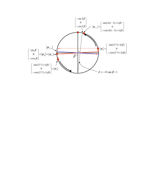
(a) No Cross until $(k-2)^{th}$ Operation

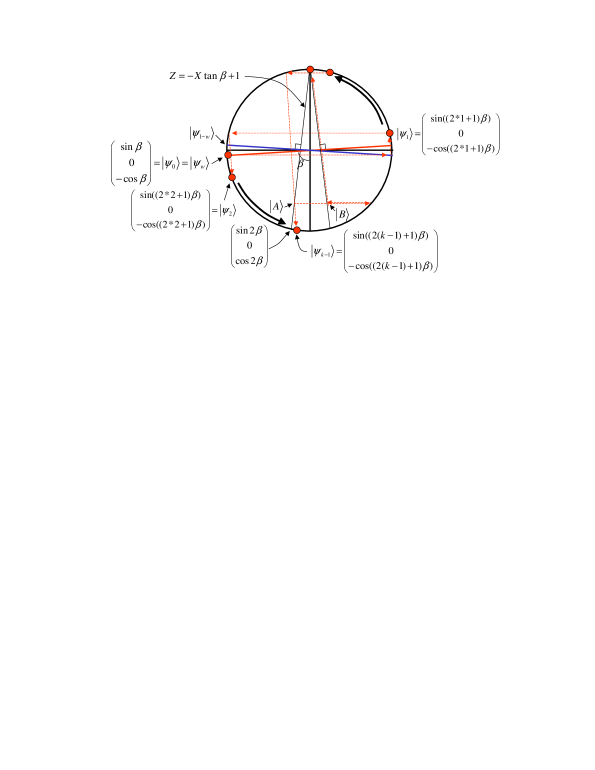
(b) First Cross in $(k-1)^{th}$ Operation

Figure 5: Correctness of Modification of Last Two Operations

4.7 Phase Conditions

Figure 6 and 7 show the trace of states for the last two operations when $k$ is even and odd, respectively. Note that we only consider the Boolean function with the smaller weight because the phase conditions are the same for the bigger weight case. At first, to rotate $|\psi_{k-2}\rangle$ state to the first cross point $|A\rangle$, $\theta_{1}$ should satisfy the following equation

$$R_{\left|\psi\right\rangle}(\theta_{1})\left({{\begin{array}[]{*{20}c}{-\sin(2k-3)\beta\hfill}\\ 0\hfill\\ {-\cos(2k-3)\beta\hfill}\\ \end{array}}}\right)=\left({{\begin{array}[]{*{20}c}{\frac{\cos(2k-2)\beta-(-1)^{k}\cos\beta}{2\sin\beta}\hfill}\\ y\hfill\\ {\frac{-\cos(2k-2)\beta-(-1)^{k}\cos\beta}{2\cos\beta}\hfill}\\ \end{array}}}\right).$$ (3)

As a result, $\theta_{1}$ should be chosen as a value to satisfy the following equation

$$\cos\theta_{1}=\frac{(-1)^{k}\cos\beta-\cos 2\beta\cos(2k-2)\beta}{\sin 2\beta\sin(2k-2)\beta}.$$ (4)

Meanwhile, the value of $y$ for the state $|A\rangle$ is calculated by $y=\sin\theta_{1}\sin(2k-2)\beta$. With the very similar approach we can find a condition for the value of $\theta_{2}$, which should satisfy the following equation

$$R_{\left|\psi\right\rangle}(\theta_{2})\left({{\begin{array}[]{*{20}c}{\frac{-\cos(2k-2)\beta+(-1)^{k}\cos\beta}{2\sin\beta}\hfill}\\ {-y\hfill}\\ {\frac{-\cos(2k-2)\beta-(-1)^{k}\cos\beta}{2\cos\beta}\hfill}\\ \end{array}}}\right)=\left({{\begin{array}[]{*{20}c}0\hfill\\ 0\hfill\\ {-(-1)^{k}\hfill}\\ \end{array}}}\right).$$ (5)

Finally, $\theta_{2}$ can be chosen, which satisfies the following equation

$$\cos\theta_{2}=\frac{(-1)^{k}\sin 2\beta(y\sin\theta_{2}-(-1)^{k}\sin\beta)}{\cos\beta\cos 2\beta-(-1)^{k}\cos(2k-2)\beta}.$$ (6)

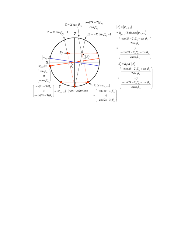
Figure 6: Last Two Operations for Even $k$

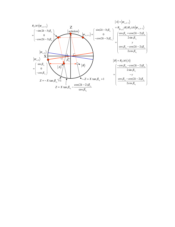
Figure 7: Last Two Operations for Odd $k$

5 Comparison with Quantum Counting Method

To argue the efficiency of our algorithm, let us refer to the existing works on quantum counting [4, 3, 2]. The existing algorithm exploits the period information of Grover iterations. From this period information, one can guess the number of solutions. Hence, as like Shor’s factoring algorithm, this is the task to find the period of Grover operations using quantum Fourier transform.

Because we proposed a way to decide the weight from given special two weights, it is meaningful to compare time complexity between our approach and the method based on quantum counting with the same promise.

5.1 Quantum Counting

Counting problem is to find the number of solutions of a given Boolean function. Meanwhile, Grover operation shows some kind period patterns with the iteration numbers. By this analysis, we can count the number of solutions with quantum Fourier transform as shown in Algorithm 5.

Algorithm 5

Quantum Counting [4, 3, 2]

Let	${\mathbf{C}}_{F}:|m\rangle\otimes|\Psi\rangle\mapsto|m\rangle\otimes({\mathbf{G}}_{F})^{m}|\Psi\rangle$
Let	${\mathbf{F}}_{P}:|k\rangle\mapsto\frac{1}{\sqrt{P\;\!}}\sum^{P-1}_{l=0}e^{2\pi\imath kl/P}\,|l\rangle$
1.	$|\Psi_{0}\rangle\ \leftarrow{\mathbf{W}}\otimes{\mathbf{W}}|0\rangle|0\rangle$
2.	$|\Psi_{1}\rangle\ \leftarrow{\mathbf{C}}_{F}\,|\Psi_{0}\rangle$
3.	$|\Psi_{2}\rangle\ \leftarrow|\Psi_{1}\rangle$ after the second register is measured (optional )
4.	$|\Psi_{3}\rangle\ \leftarrow{\mathbf{F}}_{P}\otimes{\mathbf{I}}|\Psi_{2}\rangle$
5.	$\tilde{f}\ \leftarrow$ measure $|\Psi_{3}\rangle$  (if $\tilde{f}>P/2$ then $\tilde{f}\leftarrow(P-\tilde{f})$)
6.	output: $\ N\sin^{2}(\tilde{f}\pi/P)$ (and $\tilde{f}$ if needed)

5.2 Exploitation and Analysis of Quantum Counting for Weight of Boolean Function

We analyze the quantum counting algorithm for three purposes. First, when a weight $w$ is given, how we can check the correctness of the given weight with how much time complexity. Second, when two weights are given, how we can decide the real weight with how much time complexity. Third, when $n$ possible weights are given, how we can find the real weight with how much time complexity.

5.2.1 Check Correctness of a Given Weight $w$

If a weight is given as $w$=sin${}^{2}\theta$, how can we check whether this is correct or incorrect and what about time complexity? Let $f=P\theta/\pi$. If $f$ were an integer, there would be two possibilities: either $f=0$ (which happens if $t=0$ or $t=N$), in which case $|\Psi_{3}\rangle=|0\rangle$, or $t>0$, in which case $|\Psi_{3}\rangle=a|f\rangle+b|P-f\rangle$, where $a$ and $b$ are complex numbers of norm $1/\sqrt{2}$ [4, 3, 2]. In other words, if we assume the value of $P$ as $k\pi/\theta$, the measured value of $\tilde{f}$ should be $k$. As a result, we can easily check whether the given weight is correct or not by measuring $|\Psi_{3}\rangle$. If the measured value is $k$, the given weight is correct, otherwise incorrect. In this case, the time complexity is $O(P)$. Meanwhile, because we already know the value of $\theta$ in the initial time, we can find the smallest integer value of $P$ as $k\frac{\pi}{\theta}$. If $\theta$ is $\frac{\pi}{a}$, then $P$ is just $ka$. Therefore, the time complexity of this case is $O(ka)$ when $\theta$ is $\frac{\pi}{a}$.

5.2.2 Decide Real Weight $w$ from Two Given Weights $w_{1}$ and $w_{2}$

From the previous section, we can know that when $w_{1}=sin^{2}\theta_{1}$($w_{2}=sin^{2}\theta_{2}$) is given, we can find the required number $P$ for $w_{1}$($w_{2}$) and the expected measured value as $k_{1}$($k_{2}$). However, when we want to decide which weight is real one, $k_{1}$ and $k_{2}$ should be different because they are the clues to distinguish. Therefore, we need to find the integer value $P$, which will be used for both two cases. Two values of $P$ are $P_{1}=k_{1}\pi/\theta_{1}$ and $P_{2}=k_{2}\pi/\theta_{2}$. Because we need to execute the algorithm only once, $P_{1}$ and $P_{2}$ should be the same. Hence, $k_{1}\pi/\theta_{1}$ should be equal to $k_{2}\pi/\theta_{2}$ and our job is to find suitable $k_{1}$ and $k_{2}$. Meanwhile, if $\theta_{1}=\pi/a_{1}$ and $\theta_{2}=\pi/a_{2}$, $P$ should be $k_{1}a_{1}=k_{2}a_{2}$. Considering the time complexity, we need to find the smallest integer value of $P$ by $P_{s}=LCM(a_{1},a_{2})$, where $LCM$ is the least common integer multiplier. Then, $k_{1}=P_{s}/a_{1}$ and $k_{2}=P_{s}/a_{2}$. Finally, with the value of $P_{s}$, we evaluate the algorithm, and if the measured value of $\tilde{f}$ is $k_{1}$, we can say that the weight is $w_{1}$. If the measured value of $\tilde{f}$ is $k_{2}$, we can say that the weight is $w_{2}$. Time complexity of this case is $LCM(a_{1},a_{2})$, where $\theta_{1}$ is $\pi/a_{1}$ and $\theta_{2}$ is $\pi/a_{2}$.

Now we need to compare our method and the above method based on quantum counting when $w_{1}+w_{2}=1$. If $w_{1}=sin^{2}(\frac{\pi}{\frac{4k+2}{k}})$ and $w_{2}=sin^{2}(\frac{\pi}{\frac{4k+2}{k+1}})=cos^{2}(\frac{\pi}{\frac{4k+2}{k}})$, our method, Algorithm 3 and 4 can decide which one is real one in $k$ many steps. On the other hand, the method based on quantum counting needs $P$ as $4k+2$ and if $\tilde{f}$ is $k$, the real weight is $w_{1}$ and if $\tilde{(}f)$ $k+1$, the real weight is $w_{2}$. From this analysis, we can know that the method based on quantum counting is less efficient than our method because the quantum counting method needs to exploit some period, which requires several Grover operations.

5.2.3 Find Real Weight $w$ from $n$ Possible Weights

We can extend the previous result to a more general case. When $n$ possible weights are given. Can we decide which weight is real one? The most important thing in this problem is to find the smallest integer value of $P_{s}=LCM(a_{1},a_{2},\cdots,a_{n})$. Then, as the same method in the previous section, $k_{i}$ should be $P_{s}/a_{i}$. From this analysis, we can find the real weight from the measured value $\tilde{f}$ as if $\tilde{f}$ is $k_{i}$ then the real weight is $w_{i}$. In this case, the time complexity is $P_{s}=LCM(a_{1},a_{2},\cdots,a_{n})$.

6 Conclusion and Open Problems

In this work, we have investigated the application of Grover operators to distinguish weight of Boolean function when two weights are given. Firstly, when we assume that the weight is the number of solutions, we found that Algorithm 3 can find the exact weight with almost certainty. Secondly, by exploiting the sure success Grover search method, we found a sure success weight decision algorithm, Algorithm 4, with modification of the last two Grover operations with phase conditions. Lastly, we have compared the proposed method to the quantum counting algorithm. Because the quantum counting algorithm needs period information, which requires more Grover operations, our method is more efficient than the quantum counting method.

On the other hand, until this work, we assume that two weights are given such as $wN$ and $(1-w)N$. How about other cases such as $w_{1}$ and $w_{2}$, where $w_{1}+w_{2}\neq 1$? Moreover, when three or more weights are given, can we find the exact weight with the similar approach? This may be attempted using the brief idea presented in Subsection 3.1.

Acknowledgment: Samuel L. Braunstein currently holds a Royal Society - Wolfson Research Merit Award. Byung-Soo Choi is supported by the Ministry of Information & Communication of Korea (IT National Scholarship Program).

References

- [1] Laurent Alonso, Edward M. Reingold, Rene Schott. Determining the Majority. Information Processing Letters, 47(5):253-255 (1993).
- [2] G. Brassard, P. Hoyer, M. Mosca, and A. Tapp. Quantum Amplitude Amplification and Estimation. quant-ph/0005055, May 2000.
- [3] G. Brassard, P. Hoyer, and A. Tapp. Quantum Counting. quant-ph/99805082, May 1998.
- [4] M. Boyer, G. Brassard, P. Hoyer and A. Tapp. Tight Bounds on Quantum Searching. Fortschr. Phys. 46 (1998) 4–5, 493–505.
- [5] D. Deutsch. Quantum theory, the Church-Turing principle and the universal quantum computer. Proc. R. Soc. Lond., Ser. A, 400(1818):97–117, 1985.
- [6] D. Deutsch and R. Jozsa. Rapid solution of problems by quantum computation. Proc. R. Soc. Lond., Ser. A, 439(1907):553–558, 1992.
- [7] F. Green and R. Pruim. Relativized Separation of EQP from . Information Processing Letters, 80(5):257–260, 2001.
- [8] L. Grover. A fast quantum mechanical algorithm for database search. In Proceedings of 28th Annual Symposium on the Theory of Computing (STOC), May 1996, pages 212–219. Available at xxx.lanl.gov/quant-ph/9605043.
- [9] P. Høyer. Arbitary Phases in Quantum Amplitude Amplification. Phys. Rev. A, 62(5):052304, 2000.
- [10] Jin-Yuan Hsieh, Kuo-Shong Wang, Che-Ming Li, Chi-Chuan Hwang. General Phase-Matching Condition for a Quantum Searching Algorithm. Phys. Rev. A, 65(3):034305, 2002.
- [11] Che-Ming Li, Jin-Yuan Hsieh. General SU(2) Formulation for Quantum Searching with Certainty. Phys. Rev. A, 65(5):052322, 2002.
- [12] Yan Song Li, Wei Lin, Zhang Hai, Yang Yan, Gui Lu Long, Chang Cun Tu. An SO(3) Picture for Quantum Searching. J. Phys. A, Math. Gen., 34:861, 2000.
- [13] G. L. Long. Grover Algorithm with Zero Theoretical Failure Rate. Phys. Rev. A, 64(2):022307, 2001.
- [14] Michele Mosca. Counting by quantum eigenvalue estimation. Theoretical Computer Science, 264(1):139–153, 2001.
- [15] Ashwin Nayak, Felix Wu. The quantum query complexity of approximating median and related statistics. Available at xxx.lanl.gov/quant-ph/9804066.
- [16] M. A. Nielsen and I. L. Chuang. Quantum Computation and Quantum Information. Cambridge University Press, 2002.
- [17] P. W. Shor. Polynomial-time algorithms for prime factorization and discrete logarithms on a quantum computer. SIAM Journal on Computing, 26(5):1484–1509, October 1997.
- [18] Yang Sun, Gui-Lu Long, Xiao Li. Phase Matching Condition for Quantum Search with a Generalized Initial State. Phys. Let. A, 294:143, 2002.